Independent confirmation and refined parameters of the hot Jupiter XO-5b¹

Abstract

We present HATNet observations of XO-5b, confirming its planetary nature based on evidence beyond that described in the announcement of Burke et al. (2008), namely, the lack of significant correlation between spectral bisector variations and orbital phase. In addition, using extensive spectroscopic measurements spanning multiple seasons, we investigate the relatively large scatter in the spectral line bisectors. We also examine possible blended stellar configurations (hierarchical triples, chance alignments) that can mimic the planet signals, and we are able to show that none are consistent with the sum of all the data. The analysis of the $S$ activity index shows no significant stellar activity. Our results for the planet parameters are consistent with values in Burke et al. (2008), and we refine both the stellar and planetary parameters using our data. XO-5b orbits a slightly evolved, late G type star with mass $M_{\star}=0.88\pm 0.03$ $M_{\sun}$, radius $R_{\star}=1.08\pm 0.04$ $R_{\sun}$, and metallicity close to solar. The planetary mass and radius are $1.059\pm 0.028\,M_{\rm J}$ and $1.109\pm 0.050\,R_{\rm J}$, respectively, corresponding to a mean density of $0.96_{-0.11}^{+0.14}\,\rm g\,cm^{-3}$. The ephemeris for the orbit is $P=4.187757\pm 0.000011\,{\rm d}$, $E=2454552.67168\pm 0.00029$ (BJD) with transit duration of $0.1307\pm 0.0013\,{\rm d}$. By measuring four individual transit centers, we found no signs for transit timing variations. The planet XO-5b is notable for its anomalously high Safronov number, and has a high surface gravity when compared to other transiting exoplanets with similar period.

1. Introduction

There are numerous dedicated transit searches surveying the sky for extrasolar planets that periodically transit across the face of their host star. Among the wide angle searches, those presenting discoveries have been TrES (Brown & Charbonneau, 2000; Dunham et al., 2004), XO (McCullough et al., 2005; Burke et al., 2007), HATNet (Bakos et al., 2002, 2004), and SuperWASP (Pollacco et al., 2006; Cameron et al., 2007). The initial high hope of finding hundreds of such planets (Horne, 2001) was followed by 5 years of poor harvest, and a steep learning curve for these, and many other projects. In retrospect we now understand that several important factors had initially been underestimated, such as the need for dedicated telescope time, optimal precision, stable instrumentation, low systematic noise, the number of false positives (Brown, 2003), optimal follow-up strategy, and access to high precision spectroscopic instruments. The last year showed an exponential rise in announcements, indicating that these dedicated efforts have started to bear fruit. In fact, they have reached a success rate such that the same object is occasionally independently found and announced by different groups (WASP-11b: West et al. (2008) = HAT-P-10b: Bakos et al. (2008)). Such scenarios are not necessarily duplication of effort. It is reassuring that completely independent discoveries, follow-up observations and analyses lead to similar parameters. They also provide an opportunity for joint analysis of all datasets. Here we report on a similar case, the confirmation of the planetary nature of the transiting object XO-5b, announced by Burke et al. (2008). The present paper provides not only strong new evidence supporting the planetary nature of the object, but also improved physical properties that aid in the comparison with theories of planet structure and formation. In § 2 we describe the details of the photometric detection. The follow-up observations, including the discussion of the bisector span measurements are presented in § 3. The subsequent steps of the analysis in order to characterize the star, orbit and the planet are discussed in § 5.

2. Photometric detection

Two telescopes of the HATNet project, namely HAT-6, stationed at Fred Lawrence Whipple Observatory (FLWO, $\lambda=111\arcdeg$W), and HAT-9, located on the rooftop of the Submillimeter Array control building at Mauna Kea, Hawaii ($\lambda=155\arcdeg$W), were used to observe HATNet field “G176” ($\alpha=07^{\rm h}28^{\rm m}$, $\delta=+37\arcdeg 30\arcmin$) on a nightly basis between 2004 November 26 and 2005 May 9. Altogether we acquired with these telescopes 2640 and 4280 frames, respectively, with exposures of 5 minutes.

A number of candidates have emerged from this field, and have been subjected to intense follow-up by larger instruments (§ 3). One candidate has become the transiting planet we call HAT-P-9b (Shporer et al., 2008). Another candidate internally labeled HTR176-002 has received extensive follow-up over the past two years. However, the large scatter in the spectral line bisectors, and their tentative correlation with orbital phase discouraged us from early announcement, and motivated us to pursue it further. Subsequently, HTR176-002 was announced as XO-5b by the XO group in 2007 May (Burke et al., 2008, hereafter B08). Nevertheless, we present here our results since they provide independent confirmation and also refine most of the parameters.

By chance, XO-5 happens to fall at the edge of field “G176” which overlaps with field “G177” ($\alpha=08^{\rm h}00^{\rm m}$, $\delta=+37\arcdeg 30\arcmin$). This field has been observed by the HATNet telescope HAT-7 and by the WHAT telescope at Wise Observatory, Israel (Shporer et al., 2006). Using these telescopes we collected 5440 and 1930 frames, respectively. Altogether we obtained $\sim 14290$ frames with photometric information on XO-5 — an unusually rich dataset compared to data available for a typical HATNet transit candidate.

The frames from field “G176” were processed and analyzed as described e.g. in Bakos et al. (2007). The light curves from this field were corrected for trends using the method of External Parameter Decorrelation (EPD, see Bakos et al., 2009), and the Trend Filtering Algorithm (TFA; Kovács et al., 2005). The light curves were then searched for periodic box-like signals using the Box Least Squares algorithm of Kovács et al. (2002). We detected a significant dip in the light curve of the $I\approx 12.17$ magnitude star GSC 02959-00729 (also known as 2MASS 07465196+3905404; $\alpha=7^{\mathrm{h}}46^{\mathrm{m}}51^{\mathrm{s}}.97$, $\delta=+39^{\circ}05^{\prime}40^{\prime\prime}.5$; J2000), with a depth of $\sim 12$ mmag. The period of the signal was $P=4.1878$ days, while the relative duration (first to last contact) of the transit events was $q\approx 0.027$, which is equivalent to a total duration of $Pq\approx 2.6$ hours (see Fig. 1a).

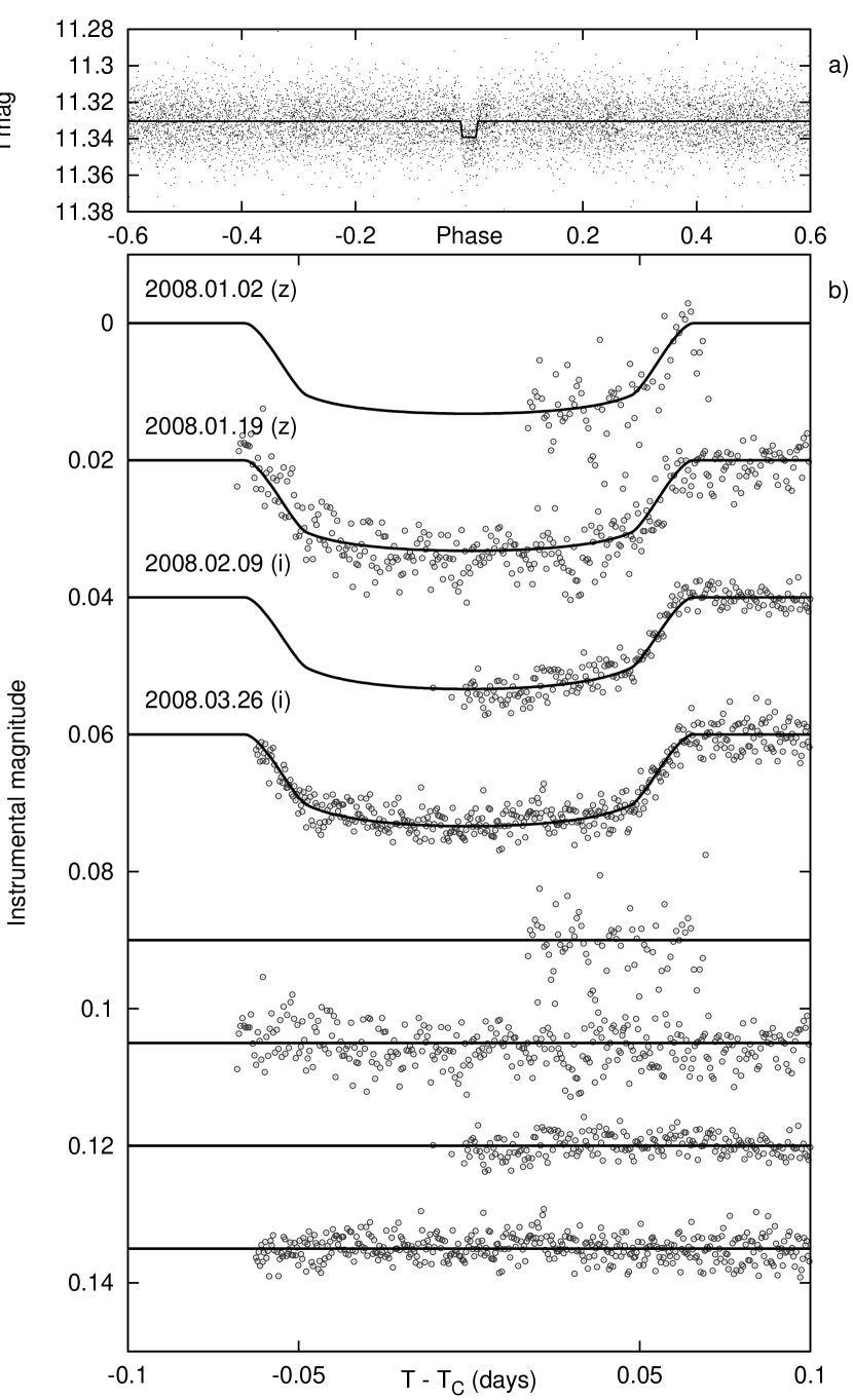
Figure 1.— (a:) The light curve of XO-5 with all 14290 points taken in the $I$ band, by the telescopes HAT-6, HAT-7, HAT-9 and WHAT. The light curve is folded with the period of $P=4.187757\pm 0.000011$ days (which is the result of the fit described in § 5). The superimposed curve shows the best fit model, neglecting limb darkening. (b:) Unbinned instrumental Sloan $z$ band and $i$ band follow-up transit photometry light curves acquired with KeplerCam on the FLWO 1.2 m telescope on 2008 January 2 ($N_{\rm tr}=0$, $z$ band), January 19 ($N_{\rm tr}=4$, $z$ band), February 9 ($N_{\rm tr}=9$, $i$ band) and March 26 ($N_{\rm tr}=20$, $i$ band). Superimposed are our best-fit transit models (§ 5).

3. Follow-up observations

3.1. Reconnaissance Spectroscopy

In order to exclude the possibility of a false planetary detection, due to the misinterpretation of a transit-like signal caused by another astrophysical scenario (such as an F + M dwarf system), we observed the candidate HTR176-002 with the CfA Digital Speedometer (Latham, 1992) on the FLWO 1.5 m Tillinghast reflector. We acquired four spectra between 2007 January and March, each with an individual precision of $0.5\,\rm km\,s^{-1}$. The observations showed a mean radial velocity of $\gamma=-10.6\,\rm km\,s^{-1}$ with an rms of $0.3\,\rm km\,s^{-1}$, therefore ruling out a low-mass stellar companion (but not a triple system), which would cause significantly higher RV variations. The spectroscopy also yielded an estimate for the projected rotational velocity and surface gravity of the star.

3.2. High S/N Spectroscopy and Subsequent Analysis

We obtained high resolution and high signal-to-noise spectra with the Keck-I telescope and HIRES instrument (Vogt et al., 1994). We acquired 17 exposures with the iodine cell, and an additional iodine-free “template”. The measurements were made between 2007 March 27 and 2008 May 17. The purpose of these observations was threefold: i) to obtain high precision radial velocity (RV) measurements, ii) to characterize the stellar properties, and iii) to check for spectral line bisector variations as an indication of blends. These steps are discussed in the following paragraphs.

As regards measuring the RV variations, the superimposed dense forest of $\mathrm{I}_{2}$ absorption lines enables us to obtain an accurate wavelength shift compared to the template observation (Marcy & Butler, 1992; Butler et al., 1996). The final RV measurements and their errors are listed in Table 1. The folded data, with our best fit (see § 5) superimposed, are plotted in Fig. 3, upper panel.

The stellar atmosphere parameters were determined using the iodine-free template spectrum. The spectral modeling was performed using the SME software (Valenti & Piskunov, 1996), with wavelength ranges and atomic line data as described by Valenti & Fischer (2005). We obtained the following initial values: effective temperature $T_{\rm eff}=5505\pm 70$ K, surface gravity $\log{g_{\star}}=4.61\pm 0.10$ (cgs), iron abundance $\mathrm{[Fe/H]}=+0.16\pm 0.06$, and projected rotational velocity $v\sin{i}=0.7\pm 0.5$ $\rm km\,s^{-1}$.

3.3. Photometric follow-up observations

We obtained follow-up photometric observations on four nights using the KeplerCam CCD on the FLWO 1.2 m telescope through Sloan $z$ and $i$ bands. The observations were performed on 2008 January 2 (partial transit), January 19 (full transit), February 9 (partial) and March 26 (full), with the total number of object frames being 114, 428, 268 and 521, respectively. The integration times used at these nights were 45, 30, 30 and 15 seconds, respectively while the readout and storage required an additional $\sim 12$ seconds per frame. The typical rms of the follow-up light curves was 2 mmag at the above cadence.

We performed aperture photometry on the calibrated frames, using an aperture series that ensures optimal flux extraction. Details on the astrometry, photometry, decorrelation for trends, etc., have been discussed in, e.g., Bakos et al. (2007). The light curves are plotted in the lower panel of Fig. 1, superimposed with the best-fit transit light curve model (see § 5).

4. Blend analysis

A stellar eclipsing binary that is unresolved from a bright source would manifest itself as a blended system with shallow photometric transits, and with RV variations that are of the same order of magnitude as one can expect from a planetary system (e.g. Queloz et al., 2001). We investigated whether such a blend is a feasible physical model for HTR176-002 in two ways: by examining the spectral line bisectors, and with a detailed modeling of the light curve under various possible blend scenarios.

For a blended eclipsing binary, in addition to the decrease in the observed RV amplitude, the spectral lines would be distorted, as quantified by the “bisector spans” (see Torres et al., 2005, 2007). If the bisector span variations correlate with the orbital phase, or the magnitude of these variations is comparable with the RV amplitude, then the system is likely to be a false positive (hierarchical triple or chance alignment with a background binary) rather than a single star with a planetary companion. In order to rule this out we derived the bisector spans by cross-correlating the iodine-free ranges of the obtained spectra against a synthetic template spectrum. We found that the standard deviation of the bisector spans is approximately $\sim 60\,\rm m\,s^{-1}$, which is comparable to the magnitude of the RV variation itself ($K=144.9\pm 2.0$ $\rm m\,s^{-1}$; see Table 3). The large bisector variations discouraged us from publication even after the first full transit follow-up light curve was obtained in January 2008, and we continued acquiring high resolution spectroscopy to establish whether there is any significant correlation between the bisectors and the orbital phase (or equivalently, with the actual RV values). In Fig. 4 we display our measurements of the bisector spans as the function of both the RV and the RV residuals from the best fit. There is no statistically significant correlation between the velocities and bisector variations, as would be expected for a blend. However, there is apparently a correlation between the RV residuals and the bisector spans. This could be due to activity on the star (e.g., spottedness), where the activity (if periodic) causes both RV and bisector variations, but in a way that is not commensurate with the orbital period of the companion. We exploit this correlation in the joint analysis of the RV and photometric data (see § 5) where we show that the unbiased residual of the RV signal can be significantly decreased with the inclusion of an additional term proportional to the bisector spans.

In order to rule out or confirm the importance of the stellar activity, we computed the Ca II emission index $S$ (Noyes et al., 1984). The derived indices are also shown in Table 1. We found that the mean value of $S=0.16\pm 0.02$ is moderately low, and the correlations between the values of $S$ and the radial velocity data or RV fit residuals are negligible (see also § 5.1).

As a further way of assessing the true nature of the candidate, we investigated possible blend configurations by performing light curve fits of our highest-quality follow-up photometry (data in the Sloan $i$ band) following the procedures described by Torres et al. (2004). Briefly, we attempted to reproduce the observed photometric variations with a model based on the EBOP binary-fitting program (Etzel, 1981; Popper & Etzel, 1981) in which three stars contribute light, two of which form an eclipsing binary with the orbital period found for XO-5. The light from the third star (the candidate) then dilutes the otherwise deep eclipses of the binary, reducing them to the level observed for HTR176-002 ($\sim$1.2% depth). The properties of the main star were adopted from the results of our analysis below, and those of the binary components (mass, size, brightness) were constrained to satisfy representative model isochrones. We explored all possible combinations for the binary components, and determined the best fits to the light curve in a chi-square sense.

The case of a hierarchical triple (all stars at the same distance) yielded an excellent fit to the photometry (see top curve in Figure 2), but implies an eclipsing binary with a primary that is half as bright as HTR176-002 itself. This is clearly ruled out by our Keck spectra and even our Digital Speedometer spectra, both of which would show obvious double lines.

We then considered scenarios in which the eclipsing binary is in the background (which would make it fainter), and is spatially unresolved. Because the proper motion of the candidate is relatively small ($\sim$30 mas yr^-1; Monet et al., 2003), the chance alignment would remain very close for decades, precluding the direct detection of the binary in archival photographic images such as those available from the Digital Sky Survey. For convenience we parametrized how far behind the eclipsing binary is placed relative to the candidate in terms of the difference in distance modulus, $\Delta m$, and we explored a wide range of values. As an example, we find that for $\Delta m=4$ (binary about 1.7 kpc behind) the best fit yields a relative brightness for the binary of only 5%, which is at or below our detection threshold of 5–10% from the Keck spectra. However, the ingress and egress are clearly too long given the quality of our photometry (Figure 2, bottom curve). For a smaller separation of $\Delta m=2$ (binary some 500 pc behind) the fit is somewhat better, though still visibly in disagreement with the observations (Figure 2, middle), and the relative brightness increases to 20%, which we would have noticed. Additional tests changing the inclination angle from the edge-on configurations considered above to lower angles did not alleviate the discrepancies.

The above modeling rules out both a hierarchical triple and a background eclipsing binary as possible alternate explanations for the photometric signals we detect. This, combined with the lack of any clear correlation between the bisector spans and the radial velocities, constitutes compelling evidence of the planetary nature of HTR176-002 = XO-5, and convinces us that the scatter in the bisector spans described above is intrinsic to the star.

Figure 2.— Blend modeling for XO-5, based on our Sloan $i$-band photometry. As examples we show the best fits corresponding to three different blend scenarios, with the bottom two displaced vertically for clarity. Top: Model corresponding to a hierarchical triple (see text), which is ruled out because the implied brightness of the eclipsing binary is so large ($\sim$50%) that our spectra would be double-lined. Middle: Model corresponding to a chance alignment with a background eclipsing binary, in which the distance modulus difference between the binary and the candidate is $\Delta m=2$. The ingress and egress are already seen to be too long, and the fit implies a relative brightness of $\sim$20% that would be easily detectable spectroscopically. Bottom: Chance alignment model with $\Delta m=4$ in which the binary is much fainter ($\sim$5%), but the best-fit model does not match the observations well. These simulations rule out background blend scenarios.

5. Analysis

In this section we describe briefly our analysis yielding the orbital, planetary and stellar parameters for the XO-5 system.

5.1. Light curve and radial velocity analysis

For the initial characterization of the spectroscopic orbit, we fitted a Keplerian model to the Keck RV data, allowing for eccentricity by including as adjustable parameters the Lagrangian orbital elements $k=e\cos\varpi$ and $h=e\sin\varpi$, in addition to a velocity offset $\gamma$, the semi-amplitude $K$ and the epoch $E$. The period $P$ was held fixed at the value found from the HATNet light curve analysis (from BLS, see above). We found that $k$ and $h$ are insignificant compared to their uncertainties ($k=-0.003\pm 0.029$, $h=-0.009\pm 0.023$), suggesting that the orbit is circular However, in the determination of the orbital and stellar parameters, we incorporated the uncertainties yielded by the $k$ and $h$ orbital elements.

We proceeded next with a joint fit using all data sets, namely, the HATNet discovery light curve, the FLWO 1.2 m follow-up light curves, and the Keck radial velocities along with the initial estimates of the spectroscopic properties derived through the SME analysis. The follow-up light curves were modeled using the analytic formalism of Mandel & Agol (2002), assuming quadratic limb darkening. The limb darkening coefficients $\gamma_{1,z}$, $\gamma_{1,i}$, $\gamma_{2,z}$ and $\gamma_{2,i}$ were taken from Claret (2004), interpolating to the values provided by the initial stellar atmospheric analysis § 3.2. The adjusted parameters for the joint fit were $T_{\mathrm{c},-270}$, the time of first transit center in the HATNet campaign, $T_{\mathrm{c},20}$, the time of the transit center at the last follow-up (on 2008 March 26), $m$, the out-of-transit magnitude of the HATNet light curve in the $I$ band, the semi-amplitude of the radial velocity $K$, the velocity offset $\gamma$, the Lagrangian orbital elements $k$ and $h$, the fractional planetary radius $p\equiv R_{\rm p}/R_{\star}$, the square of the impact parameter $b^{2}$, the quantity $\zeta/R_{\star}=(2\pi/P)(a/R_{\star})(1-b^{2})^{-1/2}\sqrt{1-e^{2}}(1+h)^{-1}$ – which is related to the duration of the transit as $T_{\rm dur}=2(\zeta/R_{\star})^{-1}$, and the out-of-transit magnitudes $m_{\rm c,0}$, $m_{\rm c,4}$, $m_{\rm c,9}$ and $m_{\rm c,20}$ for the four follow-up light curves. See Pál et al. (2008) for a detailed discussion about the advantages of this set of parameters. The initial values were based on the BLS analysis, and our initial characterization of the orbit. To obtain the best-fit values, we utilized the downhill simplex algorithm (see Press et al., 1992). The uncertainties and the correlations were determined using the Markov Chain Monte-Carlo method (Ford, 2006) which yields the a posteriori distribution of the adjusted values.

As mentioned in § 4, we found that there is a significant correlation between the RV residuals and the bisector spans. This suggests it might be possible to improve the RV fit by including an additional term to account for this correlation. We therefore expanded the model for the velocity variation to

$$v_{i}=\gamma+K\cdot{\rm RV_{0}}\left(\frac{2\pi(t_{i}-E)}{P},k,h\right)+C_{\rm BS}b_{i}$$ (1)

where ${\rm RV_{0}}(\cdot,\cdot,\cdot)$ represents the base function for the radial velocity variations and $b_{i}$ is the actual bisector span variation for the $i$-th measurement. We found that when omitting the last term the unbiased residual is $8.8$ ${\rm m\,s}^{-1}$, whereas its inclusion leads to decreased residuals of $4.6$ ${\rm m\,s}^{-1}$, nearly a factor of two better. We tested also whether the inclusion of a similar term in Eq. (1) proportional to the stellar activity index (with a coefficient $C_{\rm S-index}$) provides any further improvement in the fit, but found that it actually degrades the residuals slightly. The final orbital and planetary parameters (and their uncertainties) derived in this paper are based on the above discussed radial velocity model function decorrelated against the bisector variations.

Table 1Relative radial velocity, bisector span and stellar activity ($S$)measurements of XO-5

BJD	RV	$\sigma_{\rm RV}$	Bisec	$\sigma_{\rm Bisec}$	$S$
($2,454,000+$)	($\rm m\,s^{-1}$)	($\rm m\,s^{-1}$)	($\rm m\,s^{-1}$)	($\rm m\,s^{-1}$)
186.94763	$269.14$	$3.21$	$41.75$	$33.63$	$0.1620$
187.94425	$-$	$-$	$35.88$	$35.33$	$0.1530$
187.95384	$226.59$	$3.08$	$-0.36$	$47.48$	$0.1598$
188.95403	$33.07$	$2.79$	$20.77$	$42.04$	$0.1589$
216.76639	$294.36$	$2.70$	$81.43$	$20.90$	$0.1549$
247.80697	$0.00$	$3.37$	$-30.10$	$45.47$	$0.1876$
248.77938	$76.84$	$3.83$	$-34.80$	$48.41$	$0.1855$
249.78531	$268.26$	$3.36$	$12.13$	$36.59$	$0.1548$
251.78153	$5.41$	$3.75$	$-110.60$	$64.06$	$0.1459$
428.02826	$8.16$	$3.02$	$100.80$	$15.23$	$0.1543$
430.12240	$301.03$	$3.71$	$94.90$	$16.46$	$0.1549$
455.97787	$222.99$	$3.41$	$93.23$	$16.03$	$0.1505$
547.92199	$224.82$	$7.25$	$-\tablenotemark{a}$	$-\tablenotemark{a}$	$0.1577$
548.81658	$79.96$	$3.08$	$82.68$	$22.18$	$0.1595$
548.89652	$65.98$	$2.84$	$73.55$	$24.33$	$0.1576$
602.74168	$193.74$	$2.61$	$59.89$	$25.39$	$0.1578$
603.74268	$15.18$	$2.83$	$60.49$	$25.44$	$0.1604$

Figure 3.— (a) Radial-velocity measurements from Keck for XO-5, along with our orbital fit (see § 5). The center-of-mass velocity $\gamma$ and the correlation correction for the bisector span variations has been subtracted. (b) Phased residuals after subtracting the orbital fit (also see § 5). The rms variation of the residuals is about $4.6$ $\rm m\,s^{-1}$. (c) Bisector spans (BS) for 16 of the Keck spectra (including the iodine-free template). Note that the scales of the panels are the same.

Table 2Stellar parameters for XO-5

Parameter	Value	Source
$T_{\rm eff}$ (K)	$5370\pm 70$	SME
$[\mathrm{Fe/H}]$	$+0.05\pm 0.06$	SME
$v\sin i$ ($\rm km\,s^{-1}$)	$0.7\pm 0.5$	SME
$M_{\star}$ ($M_{\sun}$)	$0.88\pm 0.03$	Y2+LC+SME
$R_{\star}$ ($R_{\sun}$)	$1.08\pm 0.04$	Y2+LC+SME
$\log{g_{\star}}$ (cgs)	$4.31\pm 0.03$	Y2+LC+SME
$L_{\star}$ ($L_{\sun}$)	$0.88\pm 0.09$	Y2+LC+SME
$M_{V}$ (mag)	$5.06\pm 0.12$	Y2+LC+SME
Age (Gyr)	$14.8\pm 2.0$	Y2+LC+SME
Distance (pc)	$260\pm 12$	Y2+LC+SME

5.2. Stellar and planetary parameters

Figure 4.— Bisector span variations as a function of the RV (left panel) and RV fit residual (right panel). The right panel shows the fit residuals when the correlation term was not included in the fit. Note that on the graphs the horizontal scales are not the same.

The stellar parameters were determined in an iterative way as follows. As pointed out by Sozzetti et al. (2007), the stellar density is a better luminosity indicator than the spectroscopic value of $\log{g_{\star}}$. In a first order approximation the density is related to the observable quantities $P$ and $a/R_{\star}$ as $\rho_{\star}=(3\pi)G^{-1}P^{-2}(a/R_{\star})^{3}$. We used the values of $T_{\rm eff}$ and $\mathrm{[Fe/H]}$ from the SME analysis, together with the distribution of $\rho_{\star}$ (derived from $a/R_{\star}$) to estimate the stellar parameters from the Yonsei-Yale evolution models, as published by Yi et al. (2001) and Demarque et al. (2004). This resulted in a posteriori distributions of those stellar parameters, including the mass, radius, age, luminosity and colors. From the mass and radius distributions, we obtained a new value and uncertainty for the stellar surface gravity: $4.31\pm 0.03$. Since this value is significantly smaller than the previous value based on the SME analysis § 3.2, we repeated the atmospheric modeling by fixing the surface gravity to the new value ($4.31\pm 0.03$), and allowing only the metallicity and effective temperature to vary. This next iteration of the SME analysis yielded $T_{\rm eff}=5370\pm 70$ K and $\mathrm{[Fe/H]}=+0.05\pm 0.06$. Based on these new atmospheric parameters, the limb darkening coefficients were re-calculated and we repeated the joint fit for the light curve and RV parameters, followed by the stellar evolution modeling once again, in the same way as discussed earlier. In this iteration the surface gravity barely changed ($\log{g_{\star}}=4.33\pm 0.04$), so the stellar previous parameters were accepted as final (Table 2). In Fig. 5, we plot the evolutionary isochrones as the function of the effective temperature and both the stellar surface gravity and $a/R_{\star}$ (these are used as luminosity indicators). The temperature, surface gravity and relative semimajor axis values discussed here are also superimposed on these isochrone plots.

Figure 5.— Stellar evolution isochrones from the Yonsei-Yale models, corresponding to ages between $2$ and $14$ Gyr (in steps of $1$ Gyr), as a function of both surface gravity (top) and normalized semimajor axis $a/R_{\star}$ (bottom). In the top panel the isochrone metallicity ($[\rm{Fe/H}]=+0.16$), spectroscopic surface gravity, and temperature are from our initial SME analysis, the latter two shown with 1-$\sigma$ and 2-$\sigma$ confidence ellipsoids. In the lower panel the metallicity ($[\rm{Fe/H}]=+0.05$), temperature, and $a/R_{\star}$ are from the iterative analysis described in the text. Note that the latter quantities result in a significantly different evolutionary state for the star.

The results from this second global fit to all the available data (photometry, radial velocities) are listed in Table 3. In addition, values for some auxiliary parameters in this fit are: $T_{\mathrm{c},-270}=2453338.22311\pm 0.00236$ (BJD), $T_{\mathrm{c},20}=2454552.67174\pm 0.00029$ (BJD), $m=11.33042\pm 0.00010$ mag and the Keck velocity offset is $\gamma=0.8\pm 0.1$ $\rm m\,s^{-1}$. The best-fit values and uncertainties for the fitted parameters are straightforward to obtain from the MC distributions. These, in turn, lead to the planetary parameters and their uncertainties by using a direct combination of the a posteriori parameter distributions of the light curve, radial velocity and stellar parameters. We find that the mass of the planet is $M_{p}=1.059\pm 0.028$ $M_{\rm J}$, the radius is $R_{p}=1.109\pm 0.050$ $R_{\rm J}$ and its density is $\rho_{p}=0.96_{-0.11}^{+0.14}$ $\rm g\,cm^{-3}$. These quantities are also collected in Table 3. The correlation coefficient $C(M_{p},R_{p})$ between the planetary mass and radius is listed as well. We also estimated the individual transit centers of the four follow-up light curves, by adjusting only the the light curve parameters ($R_{\rm p}/R_{\star}$, $b^{2}$, $\zeta/R_{\star}$, out-of-transit magnitudes) while the transit centers were not constrained by a given epoch and period. We obtained that the individual transit centers do not differ significantly from the interpolated transit centers (derived from the results of the joint fit), i.e. the available data do not show any signs for transit timing variations. The independently fitted transit centers for the events $N_{\rm tr}=0$, $N_{\rm tr}=4$ and $N_{\rm tr}=20$ differ from the linearly interpolated values by less than $1.5$-$\sigma$, and the difference at the event $N_{\rm tr}=9$ is nearly $2.3$-$\sigma$. The independently fitted and the interpolated transit instants are shown in Table 4.

Using our best fit model, we also checked the amplitude of the out-of-transit variations of the HATNet light curve, by performing a Fourier analysis on the fit residuals. We found no significant variation in the stellar flux, and all Fourier amplitudes were less than $0.7$ mmag. This estimation gives an upper limit for the stellar activity, and is in line with the small $S$ values derived from spectroscopy ($S\lesssim 0.186$, see Table 1). It is somewhat surprising that in spite of the small activity based on the spectroscopic $S$ index, the light curve out-of-transit variation, and the low $v\sin{i}$ rotational velocity of the star, the bisector spans exhibit such a large scatter.

The Yonsei-Yale evolutionary models also provide the absolute magnitudes and colors for different photometric bands. We compared the $V-I$ model color with the observed TASS color (see Droege et al., 2006). Since $(V-I)_{\rm YY}=0.815\pm 0.016$ and $(V-I)_{\rm TASS}=0.82\pm 0.09$, we conclude that the star is not significantly affected by interstellar reddening (also note the Galactic latitude of XO-5, which is $b=26^{\circ}.9$). Therefore, for the distance determination we use the distance modulus $V_{\rm TASS}-M_{V}=7.18\pm 0.13$, which corresponds to $d=260\pm 12$ pc.

Table 3Orbital and planetary parameters

Parameter	Value
Light curve parameters
$P$ (days)	$4.187757\pm 0.000011$
$E$ (${\rm BJD}$)	$2454552.67168\pm 0.00029$
$T_{14}$ (days)	$0.1307\pm 0.0013$
$T_{12}=T_{34}$ (days)	$0.0175\pm 0.0013$
$\zeta/R_{\star}$ ($\mathrm{day^{-1}}$)	$17.779\pm 0.091$
$a/R_{\star}$	$9.67\pm 0.35$
$R_{p}/R_{\star}$	$0.1050\pm 0.0009$
$b\equiv a\cos i/R_{\star}$	$0.562_{-0.052}^{+0.033}$
$i$ (deg)	$86.7\pm 0.4$ 0
Spectroscopic parameters
$K$ ($\rm m\,s^{-1}$)	$144.9\pm 2.0$
$C_{\rm BS}$	$0.125\pm 0.025$
$C_{\rm S-index}$	$0$ (adopted)
$k\equiv e\,\cos\omega$	$+0.008\pm 0.010$
$h\equiv e\,\sin\omega$	$+0.010\pm 0.013$
Planetary parameters
$M_{p}$ ($M_{\rm J}$)	$1.059\pm 0.028$
$R_{p}$ ($R_{\rm J}$)	$1.109\pm 0.050$
$C(M_{p},R_{p})$	$0.23$
$\rho_{p}$ ($\rm g\,cm^{-3}$)	$0.96_{-0.11}^{+0.14}$
$a$ (AU)	$0.0488\pm 0.0006$
$\log g_{p}$ (cgs)	$3.33\pm 0.04$
$T_{\rm eq}$ (K)	$1221\pm 27$
$\Theta$	$0.105\pm 0.005$

Table 4Individual transit center measurements

Event	$T_{\rm C}(BJD)\tablenotemark{a}$	$T_{\rm C}(BJD)\tablenotemark{b}$
#	(2,454,000$+$)	(2,454,000$+$)
0	$468.91868\pm 0.00181$	$468.91666\pm 0.00028$
4	$485.66932\pm 0.00058$	$485.66768\pm 0.00028$
9	$506.60475\pm 0.00057$	$506.60645\pm 0.00027$
20	$552.67152\pm 0.00041$	$552.67174\pm 0.00029$

Figure 6.— (a): Safronov number vs. equilibrium temperature for the known transiting extrasolar planets. XO-5b is marked with a larger dot and it is located at the upper envelope of the Class I distribution of planets (XO-5b $>0.05$). (b): Surface gravities as the function of the orbital period for the known extrasolar planets. With its relatively high surface gravity and orbital period, XO-5b falls slightly off the main distribution.

6. Discussion

In this paper we have described our independent detection of the transiting planet XO-5b using the HATNet observations. A significant component of our effort has been to examine possible astrophysical false positives and to model the data in detail in order to rule them out. In this way we have provided new and crucial support for the planetary nature of the object. We also present refined values for the system parameters. It is reassuring that the planetary parameters in B08 and this work are consistent within 1-$\sigma$. This, however, is somewhat coincidental, since the stellar parameters are quite different. Based on our SME analysis, we derive a lower effective temperature ($T_{\rm eff}$= $5370\pm 70$ K as compared to $5510\pm 44$ K in B08), and a lower metallicity ($\mathrm{[Fe/H]}=+0.05\pm 0.06$ vs. $0.25\pm 0.03$). The difference is attributed to our iterations on the SME analysis and the transit-fitting, using the $a/R_{\star}$ based mean stellar density as a luminosity indicator, and fixing the corresponding $\log{g_{\star}}$ in the SME analysis (i.e. solving only for $\mathrm{[Fe/H]}$ and $T_{\rm eff}$). We derive a smaller stellar mass: $0.88\pm 0.03\,M_{\sun}$ vs. $1.0\pm 0.03,M_{\sun}$, based on the same Yi et al. (2001) isochrones. Due to the high precision photometric and RV data, we are able to refine the planetary and orbital parameters of the system, and decrease the uncertainties typically by a factor of $\sim 2-3$.

Based on the models of Liu et al. (2008), after re-scaling the semi-major axis to match the insolation flux XO-5b would have if it orbited a G2V dwarf ($a_{equiv}=0.05313$ AU), the measured mass and radius of XO-5b require a small core to be consistent with theory even if no internal heating is assumed. Using the work of Fortney et al. (2007), XO-5b is consistent with a 300 Myr old planet with a 50 $M_{\earth}$ core, a 1 Gyr old planet with a 25 $M_{\earth}$ core, or a 4.5 Gyr planet with a core smaller than 10 $M_{\earth}$ mass. The incident flux on XO-5b is $\sim 4.83\cdot 10^{8}\rm erg\,s^{-1}\,cm^{-2}$. This corresponds to a pL class planet, based on the definitions of Fortney et al. (2008), although it falls fairly close to the transition area between the pL and pM classes.

We confirm that the planet has a remarkably high Safronov number, $\Theta\equiv 1/2(V_{esc}/V_{orb})^{2}=0.105\pm 0.005$, placing it at the high end of the Class I planets as defined by Hansen & Barman (2007). The plot of the Safronov numbers for the known TEPs as a function of equilibrium temperature is displayed on Fig. 6a. We also confirm that XO-5b has an anomalously high surface gravity, as compared to other TEPs with similar period (Southworth, Wheatley, & Sams, 2007).

Altogether, XO-5 appears to be an interesting system exhibiting a number of anomalies including non-trivial bisector span variations, and anomalously high Safronov number and surface gravity. Future observations and theoretical work are required to understand these properties.

References

- Alonso et al. (2004) Alonso, R., et al. 2004, ApJ, 613, L153
- Bakos et al. (2002) Bakos, G. Á., Lázár, J., Papp, I., Sári, P., & Green, E. M. 2002, PASP, 114, 974
- Bakos et al. (2004) Bakos, G. Á., Noyes, R. W., Kovács, G., Stanek, K. Z., Sasselov, D. D., & Domsa, I. 2004, PASP, 116, 266
- Bakos et al. (2007) Bakos, G. Á., et al. 2007, ApJ, 670, 826
- Bakos et al. (2008) Bakos, G. Á., et al. 2008, ApJ, submitted (arXiv:0809.4295)
- Bakos et al. (2009) Bakos, G. Á., et al. 2009, ApJ, submitted (arXiv:0901.0282)
- Brown & Charbonneau (2000) Brown T. M. & Charbonneau D. 2000, In Disks, Planetesimals, and Planets (F. Garzón et al., eds.), pp. 584-589. ASP Conf. Series, San Francisco.
- Brown (2003) Brown, T. M. 2003, ApJ, 593, L125
- Burke et al. (2007) Burke, C. J., et al. 2007, ApJ, 671, 2115
- Burke et al. (2008) Burke, C. J. et al. 2008, ApJ, submitted (arXiv:0805.2399)
- Butler et al. (1996) Butler, R. P., Marcy, G. W., Williams, E., McCarthy, C., Dosanjh, P., & Vogt, S. S. 1996, PASP, 108, 500
- Claret (2004) Claret, A. 2004, A&A, 428, 1001
- Cameron et al. (2007) Cameron, A. C., et al. 2007, MNRAS, 375, 951
- Demarque et al. (2004) Demarque, P., Woo, J.-H., Kim, Y.-C., & Yi, S. K. 2004, ApJS, 155, 667
- Droege et al. (2006) Droege, T. F., Richmond, M. W., & Sallman, M. 2006, PASP, 118, 1666
- Dunham et al. (2004) Dunham, E. W., Mandushev, G. I., Taylor, B. W., & Oetiker, B. 2004, PASP, 116, 1072
- Etzel (1981) Etzel, P. B. 1981, Photometric and Spectroscopic Binary Systems (Dordrecht: Reidel), 65
- Ford (2006) Ford, E. 2006, ApJ, 642, 505
- Fortney et al. (2007) Fortney, J. J., Marley, M. S., & Barnes, J. W. 2007, ApJ, 659, 1661
- Fortney et al. (2008) Fortney, J. J., Lodders, K., Marley, M. S., & Freedman, R. S. 2008, ApJ, 678, 1419
- Hansen & Barman (2007) Hansen, B. M. S. & Barman, T. 2007, ApJ, .671, 861
- Horne (2001) Horne, K. 2001, Techniques for the Detection of Planets and Life beyond the Solar System, 5
- Kovács et al. (2002) Kovács, G., Zucker, S., & Mazeh, T. 2002, A&A, 391, 369
- Kovács et al. (2005) Kovács, G., Bakos, G. Á., & Noyes, R. W. 2005, MNRAS, 356, 557
- Latham (1992) Latham, D. W. 1992, in IAU Coll. 135, Complementary Approaches to Double and Multiple Star Research, ASP Conf. Ser. 32, eds. H. A. McAlister & W. I. Hartkopf (San Francisco: ASP), 110
- Liu et al. (2008) Liu, X., Burrows, A., & Ibgui, L. 2008, astroph/0805.1733
- Mandel & Agol (2002) Mandel, K., & Agol, E. 2002, ApJ, 580, L171
- Mandushev et al. (2007) Mandushev, G. et al. 2007, ApJ, 667, L195
- Marcy & Butler (1992) Marcy, G. W., & Butler, R. P. 1992, PASP, 104, 270
- McCullough et al. (2005) McCullough, P. R., Stys, J. E., Valenti, J. A., Fleming, S. W., Janes, K. A., & Heasley, J. N. 2005, PASP, 117, 783
- McCullough et al. (2006) McCullough, P. R., et al. 2006, ApJ, 648, 1228
- Monet et al. (2003) Monet, D. G., Levine, S. E., Casian, B. et al. 2003, AJ, 125, 984
- Noyes et al. (1984) Noyes, R. W., Hartmann, L. W., Baliunas, S. L., Duncan, D. K. & Vaughan, A. H. 1984, ApJ, 279, 763
- Pál & Bakos (2006) Pál, A., & Bakos, G. Á. 2006, PASP, 118, 1474
- Pál et al. (2008) Pál, A. et al. 2008, ApJ, 680, 1450
- Pollacco et al. (2006) Pollacco, D. et al. 2006, PASP, 118, 1407
- Popper & Etzel (1981) Popper, D. M., & Etzel, P. B. 1981, AJ, 86, 102
- Press et al. (1992) Press, W. H., Teukolsky, S. A., Vetterling, W. T. & Flannery, B. P., 1992, Numerical Recipes in C: the art of scientific computing, Second Edition, Cambridge University Press
- Queloz et al. (2001) Queloz, D. et al. 2001, A&A, 379, 279
- Shporer et al. (2006) Shporer, A., Mazeh, T., Moran, A., Bakos, G., Kovacs, G., & Mashal, E. 2006, Tenth Anniversary of 51 Peg-b: Status of and prospects for hot Jupiter studies, 196
- Shporer et al. (2008) Shporer, A. et al. 2008, ApJ, submitted (arXiv:0806.4008)
- Sozzetti et al. (2007) Sozzetti, A. et al. 2007, ApJ, 664, 1190
- Street et al. (2003) Street, R. A., et al. 2003, Scientific Frontiers in Research on Extrasolar Planets, 294, 405
- Torres et al. (2005) Torres, G., Konacki, M., Sasselov, D. D., & Jha, S. 2005, ApJ, 619, 558
- Torres et al. (2004) Torres, G., Konacki, M., Sasselov, D. D., & Jha, S. 2005, ApJ, 614, 979
- Torres et al. (2007) Torres, G. et al. 2007, ApJ, 666, 121
- Southworth, Wheatley, & Sams (2007) Southworth, J., Wheatley, P. J., & Sams, G. 2007, MNRAS, 379, 11
- Valenti & Piskunov (1996) Valenti, J. A., & Piskunov, N. 1996, A&AS, 118, 595
- Valenti & Fischer (2005) Valenti, J. A., & Fischer, D. A. 2005, ApJS, 159, 141
- Vogt et al. (1994) Vogt, S. S. et al. 1994, Proc. SPIE, 2198, 362
- West et al. (2008) West, R. G. et al. 2008, A&A, submitted (http://exoplanet.eu/papers/wasp11.pdf)
- Yi et al. (2001) Yi, S. K. et al. 2001, ApJS, 136, 417