Invisibility and Inverse Problems

Abstract

We describe recent theoretical and experimental progress on making objects invisible. Ideas for devices that would have once seemed fanciful may now be at least approximately realized physically, using a new class of artificially structured materials, metamaterials. The equations that govern a variety of wave phenomena, including electrostatics, electromagnetism, acoustics and quantum mechanics, have transformation laws under changes of variables which allow one to design material parameters that steer waves around a hidden region, returning them to their original path on the far side. Not only are observers unaware of the contents of the hidden region, they are not even aware that something is being hidden; the object, which casts no shadow, is said to be cloaked. Proposals for, and even experimental implementations of, such cloaking devices have received the most attention, but other devices having striking effects on wave propagation, unseen in nature, are also possible. These designs are initially based on the transformation laws of the relevant PDEs, but due to the singular transformations needed for the desired effects, care needs to be taken in formulating and analyzing physically meaningful solutions. We recount the recent history of the subject and discuss some of the mathematical and physical issues involved.

1 Introduction

Invisibility has been a subject of human fascination for millennia, from the Greek legend of Perseus versus Medusa to the more recent The Invisible Man and Harry Potter. Over the years, there have been occasional scientific prescriptions for invisibility in various settings, e.g., [56, 11]. However, since 2005 there has been a wave of serious theoretical proposals [4, 83, 79, 73, 93] in the physics literature, and a widely reported experiment by Schurig et al. [99], for cloaking devices – structures that would not only make an object invisible but also undetectable to electromagnetic waves, thus making it cloaked. The particular route to cloaking that has received the most attention is that of transformation optics [116], the design of optical devices with customized effects on wave propagation, made possible by taking advantage of the transformation rules for the material properties of optics: the index of refraction $n(x)$ for scalar optics, governed by the Helmholtz equation, and the electrical permittivity $\varepsilon(x)$ and magnetic permeability $\mu(x)$ for vector optics, as described by Maxwell’s equations. It is this approach to cloaking, and other novel effects on wave propagation, that we will examine here.

As it happens, two papers appeared in the same 2006 issue of Science with transformation optics-based proposals for cloaking. Leonhardt [73] gave a description, based on conformal mapping, of inhomogeneous indices of refraction $n$ in two dimensions that would cause light rays to go around a region and emerge on the other side as if they had passed through empty space (for which $n(x)\equiv 1$). On the other hand, Pendry, Schurig and Smith [93] gave a prescription for values of $\varepsilon$ and $\mu$ yielding a cloaking device for electromagnetic waves, based on the fact that $\varepsilon$ and $\mu$ transform nicely under changes of variables, cf. (25). In fact, this construction used the same singular transformation (6) as had been used three years earlier [44, 45] to describe examples of nondetectability in the context of Calderón’s Problem for conductivity, which transforms in the same way as $\varepsilon$ and $\mu$.

We briefly outline here the basic ideas of transformation optics, in the context of electrostatics, leading to a theoretical blueprint of a conductivity that cloaks an object from observation using electrostatic measurements [44, 45]. Given that the invariance of the underlying equation is a crucial ingredient of transformation optics it is natural to set Calderón’s problem on a compact Riemannian manifold with boundary, $(M,g)$ with $g$ the Riemannian metric and boundary $\partial M$ where the observations are made. The Laplace-Beltrami operator associated to $g$ is given in local coordinates by

$$\Delta_{g}u=\frac{1}{\sqrt{|g|}}\sum^{n}_{i,j=1}\frac{\partial}{\partial x_{i}}\left(\sqrt{|g|}g^{ij}\frac{\partial u}{\partial x_{j}}\right)$$ (1)

where $(g^{ij})$ is the matrix inverse of the metric tensor $(g_{ij})$ and $|g|=\hbox{det}\,g$. Let us consider the Dirichlet problem associated to (1),

$$\Delta_{g}u=0\hbox{ on }M,\quad u|_{\partial M}=f.$$ (2)

We define the Dirichlet-to-Neumann (DN) map in this case by

$$\Lambda_{g}(f)=\sum^{n}_{i,j=1}\left.\left(\nu_{i}g^{ij}\sqrt{|g|}\frac{\partial u}{\partial x_{j}}\right)\right|_{\partial M}\quad$$ (3)

where $\nu$ denotes the unit outer normal. Calderón’s (inverse) problem, the question of whether one can recover $g$ from $\Lambda_{g}$, has been the subject of a tremendous amount of work over the last quarter century. In Sec. 2, we briefly summarize the history and current status of this problem.

Given the invariant formulation of the DN map, it is straightforward to see that

$$\Lambda_{\psi^{\ast}g}=\Lambda_{g}$$ (4)

for any $C^{\infty}$ diffeomorphism $\psi$ of $\overline{M}$ which is the identity on the boundary. As usual, $\psi^{\ast}g$ denotes the pull back of the metric $g$ by the diffeomorphism $\psi$. For domains in Euclidean space of dimension $n\geq 3$, the metric $g$ corresponds to an anisotropic conductivity $\sigma$, represented by the symmetric matrix-valued function

$$\sigma^{ij}=|g|^{1/2}g^{ij}.$$ (5)

The DN map sends the voltage potential at the boundary to the induced current flux.

The invariance (4) can be considered as a weak form of invisibility. However, although the (generally distinct) media represented by $g$ and $\psi^{*}g$ are indistinguishable by boundary observations, nothing has yet been hidden. In cloaking, we are looking for a way to hide from boundary measurements both an object enclosed in some domain $D$ and the fact that it is being hidden. Suppose now that an object we want to cloak is enclosed in the ball of radius one, $B(0,1)$, and that we measure the DN map on the boundary of the the ball of radius two, $B(0,2)$. Motivated by degenerations of singular Riemannian manifolds (see Sec. 3) consider the following singular transformation stretching (or “blowing up”) the origin to the ball $\overline{B}(0,1)$:

$$F_{1}:B(0,2)\setminus\{0\}\to B(0,2)\setminus\overline{B}(0,1),$$ (6)

$$F_{1}(x)=(\frac{|x|}{2}+1)\frac{x}{|x|},\quad 0<|x|<2.$$

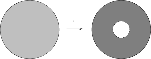
Figure 1: Map $F_{1}:B(0,2)\setminus\{0\}\to B(0,2)\setminus\overline{B}(0,1)$

Also note that the metric $\widetilde{g}=(F_{1})_{*}g_{0}$, where $(F_{1})_{*}=(F_{1}^{-1})^{*}$ and $g_{0}$ is the Euclidean metric, is singular on the unit sphere $\mathbb{S}^{n-1}$, the interface between the cloaked and uncloaked regions, which we call the cloaking surface. In fact, the conductivity $\widetilde{\sigma}$ associated to this metric by (5) has zero and/or infinite eigenvalues (depending on the dimension) as $r\searrow 1$. In $\mathbb{R}^{3}$, $\widetilde{\sigma}$ is given in spherical coordinates $(r,\phi,\theta)\mapsto(r\sin\theta\cos\phi,r\sin\theta\sin\phi,r\cos\theta)$ by

$$\widetilde{\sigma}=\left(\begin{array}[]{ccc}2(r-1)^{2}\sin\theta&0&0\\ 0&2\sin\theta&0\\ 0&0&2(\sin\theta)^{-1}\\ \end{array}\right),\quad 1<|x|\leq 2.$$ (7)

Note that $\widetilde{\sigma}$ is singular (degenerate) on the sphere of radius $1$ in the sense that it is not bounded from below by any positive multiple of the identity matrix $I$. (See [62] for a similar calculation.)

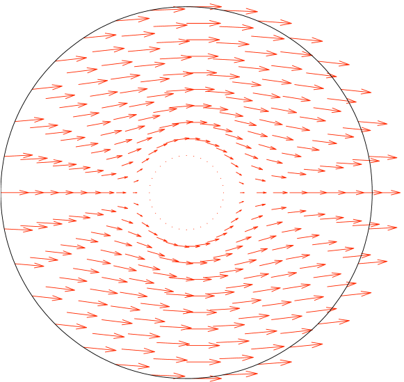
Figure 2: Analytic solutions for the currents

The currents associated to this singular conductivity on $B(0,2)\setminus\overline{B}(0,1)$ are shown in Fig. 2. No currents originating at $\partial B(0,2)$ have access to the region $B(0,1)$, so that (heuristically) if the conductivity is changed in $B(0,1)$, the measurements on the boundary $\partial B(0,2)$ do not change. Any object in $B(0,1)$ is both unaffected and undetectable by currents from the outside. Moreover, all voltage-to-current measurements made on $\partial B(0,2)$ give the same results as the measurements on the surface of a ball filled with homogeneous, isotropic material. The object is said to be cloaked, and the structure on $B(0,2)\setminus\overline{B}(0,1)$ producing this effect is said to be a cloaking device.

However, this intuition needs to be supported by rigorous analysis of the solutions on the entire region $B(0,2)$. If we consider a singular metric $\widetilde{g}$ defined by $(F_{1})_{*}(g_{0})$ on $B(0,2)\setminus\overline{B}(0,1)$, an arbitrary positive-definite symmetric metric on $B(0,1)$, and $H^{1}(B(0,2))$ smooth solutions of the conductivity equation, it was shown in [44, 45] that, for $n\geq 3$, the following theorem holds.

Theorem 1.1

$\Lambda_{\widetilde{g}}=\Lambda_{g_{0}}.$

In other words the boundary observations for the singular metric $\widetilde{g}$ are the same as the boundary observations for the Euclidean metric; thus, any object in $B(0,1)$ is invisible to electrostatic measurements. We remark here that the measurements of the DN map or “near field” are equivalent to scattering or “far field” information [12]. Also, see [62] for the planar case, $n=2$.

In the proof of Thm. 1.1 one has to pay special attention to what is meant by a solution of the Laplace-Beltrami equation (2) with singular coefficients. In [44, 45], we considered functions that are bounded and in the Sobolev space $H^{1}(B(0,2))$, and are solutions in the sense of distributions. Later, we will also consider more general solutions.

The proof of Theorem 1.1 has two ingredients, which are also the main ideas behind transformation optics:

• The invariance of the equation under transformations, i.e., identity (4).

• A (quite standard) removable singularities theorem: points are removable singularities of bounded harmonic functions.

The second point implies that bounded solutions of the Laplace-Beltrami equation with the singular metric indicated above on the annulus $B(0,2)\setminus B(0,1)$ are equivalent to bounded harmonic functions on the whole ball $B(0,2)$. This shows that any $H^{1}$ solution $u$ to the equation (1) is constant on the ball of radius 1 with the constant the value of the corresponding harmonic function $v(0)$ with $v=u\circ F_{1}.$

The 2003 papers [44, 45] were intended to give counterexamples to uniqueness in Calderón’s problem when the anisotropic conductivity is allowed to be only positive semi-definite. In the summer of 2006, Bob Kohn called our attention to the paper [93] where the same transformation $F_{1}$ was used to propose cloaking for Maxwell’s equations, justified by the analogue of (4). In fact the electrical permittivity and magnetic permeability in the blueprint for a cloaking device given in [93] are

$$(\widetilde{\varepsilon}^{ij})=(\widetilde{\mu}^{ij})=(|\widetilde{g}|^{1/2}\widetilde{g}^{ij})$$ (8)

with $\widetilde{g}=(F_{1})_{*}g_{0}$. The proposal of [73] (appearing in the same issue of Science!) uses a different construction in two dimensions with explaining the behavior of the light rays but not the electromagnetic waves. The argument of [93] is only valid outside the cloaked region; it doesn’t take into account the behavior of the waves on the entire region, including the cloaked region and its boundary, the cloaking surface. In fact, the sequel [27], which gave numerical simulations of the electromagnetic waves in the presence of a cloak, states: “Whether perfect cloaking is achievable, even in theory, is also an open question”. In [35] we established that perfect cloaking is indeed mathematically possible at any fixed frequency.

Before we discuss the paper [35] and other developments, we would like to point out that it is still an open question whether visual cloaking is feasible in practice, i.e., whether one can realize such theoretical blueprints for cloaking over all, or some large portion of, the visible spectrum. The main experimental evidence has been at microwave frequencies [99], with a limited version at a visible frequency [104]. While significant progress has been made in the design and fabrication of metamaterials, including recently for visible light [78, 102], metamaterials are nevertheless very dispersive and one expects them to work only for a narrow range of frequencies. Even theoretically, one can unfortunately not expect to actually cloak electromagnetically at all frequencies, since the group velocity cannot be faster than the velocity of light in a vacuum.

In [35], Thm. 1.1 was extended to the Helmholtz equation, which models scalar optics (and acoustic waves [23, 29] and quantum waves under some conditions [125]), and Maxwell’s equations, corresponding to invisibility for general electromagnetic waves. The case of acoustic or electromagnetic sources inside and outside the cloaked region, leading to serious obstacles to cloaking for Maxwell’s equations, was also treated.

In Sec. 4.3, we consider acoustic cloaking, i.e., cloaking for the Helmholtz equation at any non-zero frequency with an acoustic source $\rho$,

$$(\Delta_{g}+k^{2})u=\rho,\quad\mbox{in }B(0,2)\,.$$ (9)

Physically, the anisotropic density is given by $|g|^{1/2}g^{ij}$ and the bulk modulus by $|g|^{1/2}.$

For acoustic cloaking, even with acoustic sources inside $B(0,1)$, we consider the same singular metric considered for electrostatics. However, we need to change the notion of a solution since for a generic frequency a $H^{1}(B(0,2))$ smooth solution of the Helmholtz equation cannot simultaneously satisfy a homogeneous Neumann condition on the surface of the cloaked region [35, Thm. 3.5] and have a Dirichlet boundary value that is a non-zero constant. We change the notion of solution for Helmholtz equation to a finite energy solution (see Sec. 4.3). The key ingredient of the rigorous justification of transformation optics is then a removable singularities theorem for the Laplacian on $H^{1}(B(0,2)\setminus 0)$.

In Sec. 4.4 we consider the case of Maxwell’s equations. In the absence of internal currents, the construction of [44, 45], called the single coating in [35], still works once one makes an appropriate definition of finite energy solutions. However, cloaking using this construction fails in the presence of sources within the cloaked region, i.e., for cloaking of active objects, due to the nonexistence of finite energy, distributional solutions. This problem can be avoided by augmenting the external metamaterial layer with an appropriately matched internal one in $D$; this is called the double coating; see Sec.  4.4.

In Sec. 5 we consider another type of transformation optics-based device, an electromagnetic wormhole. The idea is to create a secret connection between two points in space so that only the incoming and the outgoing waves are visible. One tricks the electromagnetic waves to behave as though they were propagating on a handlebody, giving the impression that the topology of space has been changed. Moreover, one can manipulate the rays travelling inside the handle to obtain various additional optical effects; see Fig. 3. Mathematically this is accomplished by using the single coating construction with special boundary conditions on the cloaking surface. The main difference is that, instead of a point, we blow up a curve, which in dimension $3$ or higher is also an $H^{1}$ removable singularity for solutions of Maxwell’s equations.

         

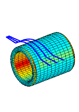
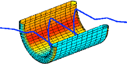
Figure 3: An electromagnetic wormhole is obtained by blowing up a metric near a curve. This corresponds to $\epsilon$ and $\mu$ on the exterior of a thickened cylinder causing electromagnetic waves to propagate as if a handle were attached to Euclidean space. Behavior of light rays: (Left) Rays travelling outside wormhole. (Right) A ray transiting wormhole.

Both the anisotropy and singularity of the cloaking devices present serious challenges in trying to physically realize such theoretical plans using metamaterials. In Sec. 7, we give a general method, isotropic transformation optics, for dealing with both of these problems; we describe it in some detail in the context of cloaking, but it should be applicable to a wider range of transformation optics-based designs.

A well known phenomenon in effective medium theory is that homogenization of isotropic material parameters may lead, in the small-scale limit, to anisotropic ones [81]. Using ideas from [2, 26] and elsewhere, we showed in [40, 41, 42] how to exploit this to find cloaking material parameters that are at once both isotropic and nonsingular, at the price of replacing perfect cloaking with approximate cloaking of arbitrary accuracy. This method, starting with transformation optics-based designs and constructing approximations to them, first by nonsingular, but still anisotropic, material parameters, and then by nonsingular isotropic parameters, seems to be a very flexible tool for creating physically realistic designs, easier to implement than the ideal ones due to the relatively tame nature of the materials needed, yet essentially capturing the desired effect on waves for all practical purposes.

In Sec. 8 we consider some further developments and open problems.

2 Visibility for electrostatics:
Calderón’s problem

Calderón’s inverse conductivity problem, which forms the mathematical foundation of Electrical Impedance Tomography (EIT), is the question of whether an unknown conductivity distribution inside a domain in $\mathbb{R}^{n}$, modelling, e.g., the Earth, a human thorax, or a manufactured part, can be determined from voltage and current measurements made on the boundary. A.P. Calderón’s motivation for proposing this problem was geophysical prospection. In the 1940’s, before his distinguished career as a mathematician, Calderón was an engineer working for the Argentinian state oil company. Apparently, Calderón had already at that time formulated the problem that now bears his name, but he did not publicize this work until thirty years later [19].

One widely studied potential application of EIT is the early diagnosis of breast cancer [25]. The conductivity of a malignant breast tumor is typically 0.2 mho, significantly higher than normal tissue, which has been typically measured at 0.03 mho. See the book [49] and the special issue of Physiological Measurement [51] for applications of EIT to medical imaging and other fields, and [13] for a review.

         

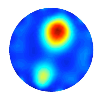
Figure 4: Left: An EIT measurement configuration for imaging objects in a tank. The electrodes used for measurements are at the boundary of the tank, which is filled with a conductive liquid. Right: A reconstruction of the conductivity inside the tank obtained using boundary measurements.   [Jari Kaipio, Univ. of Kuopio, Finland; by permission.]

For isotropic conductivities this problem can be mathematically formulated as follows: Let $\Omega$ be the measurement domain, and denote by $\sigma(x)$ the coefficient, bounded from above and below by positive constants, describing the electrical conductivity in $\Omega$. In $\Omega$ the voltage potential $u$ satisfies a divergence form equation,

$$\nabla\cdot\sigma\nabla u=0.$$ (10)

To uniquely fix the solution $u$ it is enough to give its value, $f$, on the boundary. In the idealized case, one measures, for all voltage distributions $u|_{\partial\Omega}=f$ on the boundary the corresponding current fluxes, $\nu\cdotp\sigma\nabla u$, over the entire boundary, where $\nu$ is the exterior unit normal to $\partial\Omega$. Mathematically this amounts to the knowledge of the Dirichlet-to-Neumann (DN) map, $\Lambda_{\sigma}$, corresponding to $\sigma$, i.e., the map taking the Dirichlet boundary values of the solution to (10) to the corresponding Neumann boundary values,

$$\Lambda_{\sigma}:\ \ u|_{\partial\Omega}\mapsto\nu\cdotp\sigma\nabla u|_{\partial\Omega}.$$ (11)

Calderón’s inverse problem is then to reconstruct $\sigma$ from $\Lambda_{\sigma}$.

In the following subsections, we give a brief overview of the positive results known for Calderón’s problem and related inverse problems.

A basic distinction, important for understanding cloaking, is between isotropic conductivities, which are scalar-valued, and anisotropic conductivities, which are symmetric matrix- or tensor-valued, modelling situations where the conductivity depends on both position and direction. Of course, an isotropic $\sigma(x)$ can be considered as anisotropic by identifying it with $\sigma(x)I_{n\times n}$.

Unique determination of an isotropic conductivity from the DN map was shown in dimension $n>2$ for $C^{2}$ conductivities in [108]. At the writing of the current paper this result has been extended to conductivities having $\frac{3}{2}$ derivatives in [14] and [92]. In two dimensions the first unique identifiability result was proven in [85] for $C^{2}$ conductivities. This was improved to Lipschitz conductivities in [15] and to merely $L^{\infty}$ conductivities in [5]. All of these results use complex geometrical optics (CGO) solutions, the construction of which we review in Sec. 2.1. We briefly discuss in Sec. 2.2 shielding, a less satisfactory variant of cloaking which is possible using highly singular isotropic materials.

In Sec. 2.3 we discuss the case of anisotropic conductivities, i.e., conductivities that may vary not only with location but also on the direction. In this case, the problem is invariant under changes of variables that are the identity at the boundary. We review the positive results that are known about the Calderón problem in this setting. The fact that the anisotropic conductivity equation is invariant under transformations plays a crucial role on the constructions of electromagnetic parameters that make objects invisible, but for those one needs to make a final leap to using singular transformations.

2.1 Complex geometrical optics solutions

In this section, we consider isotropic conductivities. If $u$ is a solution of (10) with boundary data $f$, the divergence theorem gives that

$$Q_{\sigma}(f):=\int_{\Omega}\sigma|\nabla u|^{2}\,dx=\int_{\partial\Omega}\Lambda_{\sigma}(f)f\,dS$$ (12)

where $dS$ denotes surface measure. In other words $Q_{\sigma}(f)$ is the quadratic form associated to the linear map $\Lambda_{\sigma}(f)$, i.e., to know $\Lambda_{\sigma}(f)$ or $Q_{\sigma}(f)$ for all $f\in H^{\frac{1}{2}}(\partial\Omega)$ is equivalent. The form $Q_{\sigma}(f)$ measures the energy needed to maintain the potential $f$ at the boundary. Calderón’s point of view in order to determine $\sigma$ in $\Omega$ was to find enough solutions $u\in H^{1}(\Omega)$ of the conductivity equation $\mbox{div}(\sigma\nabla u)=0$ so that the functions $|\nabla u|^{2}$ span a dense set (in an appropriate topology). Notice that the DN map (or $Q_{\sigma}$) depends non-linearly on $\sigma.$ Calderón considered the linearized problem at a constant conductivity. A crucial ingredient in his approach is the use of the harmonic complex exponential solutions:

$$u=e^{x\cdot\rho},\mbox{ where }\rho\in{\mathbb{C}}^{n}\mbox{ with }\rho\cdot\rho=0.$$ (13)

Sylvester and Uhlmann [108] constructed in dimension $n\geq 2$ complex geometrical optics (CGO) solutions of the conductivity equation for $C^{2}$ conductivities similar to Calderón’s. This can be reduced to constructing solutions in the whole space (by extending $\sigma=1$ outside a large ball containing $\Omega$) for the Schrödinger equation with potential. We describe this more precisely below.

Let $\sigma\in C^{2}(\mathbb{R}^{n})$, $\sigma$ strictly positive in $\mathbb{R}^{n}$ and $\sigma=1$ for $|x|\geq R$, for some $R>0$. Let $L_{\sigma}u=\nabla\cdot\sigma\nabla u$. Then we have

$$\sigma^{-\frac{1}{2}}L_{\sigma}\left(\sigma^{-\frac{1}{2}}v\right)=(\Delta-q)v,$$ (14)

where

$$q=\frac{\Delta\sqrt{\sigma}}{\sqrt{\sigma}}.$$ (15)

Therefore, to construct solutions of $L_{\sigma}u=0$ in $\mathbb{R}^{n}$ it is enough to construct solutions of the Schrödinger equation $(\Delta-q)v=0$ with $q$ of the form (15). The next result proven in [108] states the existence of complex geometrical optics solutions for the Schrödinger equation associated to any bounded and compactly supported potential.

Theorem 2.1

Let $q\in L^{\infty}(\mathbb{R}^{n})$, $n\geq 2$, with $q(x)=0$ for $|x|\geq R>0$. Let $-1<\delta<0.$ There exists $\epsilon(\delta)$ and such that for every $\rho\in{\mathbb{C}}^{n}$ satisfying

$$\rho\cdot\rho=0$$

and

$${\|(1+|x|^{2})^{1/2}q\|_{L^{\infty}(\mathbb{R}^{n})}+1\over|\rho|}\leq\epsilon$$

there exists a unique solution to

$$(\Delta-q)v=0$$

of the form

$$v=e^{x\cdot\rho}(1+\psi_{q}(x,\rho))$$ (16)

with $\psi_{q}(\cdot,\rho)\in L^{2}_{\delta}(\mathbb{R}^{n})$. Moreover $\psi_{q}(\cdot,\rho)\in H^{2}_{\delta}(\mathbb{R}^{n})$ and, for $0\leq s\leq 1$, there exists $C=C(n,s,\delta)>0$ such that

$$\|\psi_{q}(\cdot,\rho)\|_{H^{s}_{\delta}}\leq\frac{C}{|\rho|^{1-s}}$$ (17)

Here

$$L^{2}_{\delta}(\mathbb{R}^{n})=\{f;\int(1+|x|^{2})^{\delta}|f(x)|^{2}dx<\infty\}$$

with the norm given by $\|f\|^{2}_{L^{2}_{\delta}}=\int(1+|x|^{2})^{\delta}|f(x)|^{2}dx$ and $H^{m}_{\delta}(\mathbb{R}^{n})$ denotes the corresponding Sobolev space. Note that for large $|\rho|$ these solutions behave like Calderón’s exponential solutions $e^{x\cdot\rho}$. The equation for $\psi_{q}$ is given by

$$(\Delta+2\rho\cdot\nabla)\psi_{q}=q(1+\psi_{q}).$$ (18)

The equation (18) is solved by constructing an inverse for $(\Delta+2\rho\cdot\nabla)$ and solving the integral equation

$$\psi_{q}=(\Delta+2\rho\cdot\nabla)^{-1}(q(1+\psi_{q})).$$ (19)

Lemma 2.2

Let $-1<\delta<0,\quad 0\leq s\leq 1$. Let $\rho\in{\mathbb{C}}^{n}\setminus 0$, $\rho\cdot\rho=0$. Let $f\in L^{2}_{\delta+1}(\mathbb{R}^{n})$. Then there exists a unique solution $u_{\rho}\in L^{2}_{\delta}(\mathbb{R}^{n})$ of the equation

$$\Delta_{\rho}u_{\rho}:=(\Delta+2\rho\cdot\nabla)u_{\rho}=f.$$ (20)

Moreover $u_{\rho}\in H^{2}_{\delta}(\mathbb{R}^{n})$ and

$$\|u_{\rho}\|_{H^{s}_{\delta}(\mathbb{R}^{n})}\leq\frac{C_{s,\delta}\|f\|_{L^{2}_{\delta+1}}}{|\rho|^{1-s}}$$

for $0\leq s\leq 2$ and for some constant $C_{s,\delta}>0$.

The integral equation (19) with Faddeev’s Green kernel [34] can then be solved in $L^{2}_{\delta}(\mathbb{R}^{n})$ for large $|\rho|$ since

$$(I-(\Delta+2\rho\cdot\nabla)^{-1}q)\psi_{q}=(\Delta+2\rho\cdot\nabla)^{-1}q$$

and $\|(\Delta+2\rho\cdot\nabla)^{-1}q\|_{L^{2}_{\delta}\to L^{2}_{\delta}}\leq\frac{C}{|\rho|}$ for some $C>0$ where $\|\cdot\|_{L^{2}_{\delta}\to L^{2}_{\delta}}$ denotes the operator norm between $L^{2}_{\delta}(\mathbb{R}^{n})$ and $L^{2}_{\delta}(\mathbb{R}^{n})$. We will not give details of the proof of Lemma 2.2 here. We refer to the papers [108, 107] .

If $0$ is not a Dirichlet eigenvalue for the Schrödinger equation we can also define the DN map

$$\Lambda_{q}(f)=\frac{\partial u}{\partial\nu}|_{\partial\Omega}$$

where $u$ solves

$$(\Delta-q)u=0;\quad u|_{\partial\Omega}=f.$$

Under some regularity assumptions, the DN map associated to the Schrödinger equation $\Delta-q$ determines in dimension $n>2$ uniquely a bounded potential; see [108] for the smooth case, [87] for $L^{\infty}$, and [20] for potentials in a Fefferman-Phong class.

The two dimensional results of [85],[15], [5] use similar CGO solutions and the $\overline{\partial}$ method in the complex frequency domain, introduced by Beals and Coifman in [9] and generalized to higher dimensions in several articles [10],[1],[86].

More general CGO solutions have been constructed in [52] of the form

$$u=e^{\tau(\phi+i\psi)}(a+r),$$ (21)

where $\nabla\phi\cdot\nabla\psi=0,|\nabla\phi|^{2}=|\nabla\psi|^{2}$ and $\phi$ is a limiting Carleman weight (LCW). Moreover $a$ is smooth and non-vanishing and $\|r\|_{L^{2}(\Omega)}=O(\frac{1}{\tau})$, $\|r\|_{H^{1}(\Omega)}=O(1)$. Examples of LCW are the linear phase $\phi(x)=x\cdot\omega,\omega\in S^{n-1},$ used in the results mentioned above, and the non-linear phase $\phi(x)=\ln|x-x_{0}|$, where $x_{0}\in{\bf R}^{n}\setminus\overline{{\rm ch\,}(\Omega)}$ ($ch(\cdot)$ denoting the convex hull) which was used in [52] for the problem where the DN map is measured in parts of the boundary. For a characterization of all the LCW in $\mathbb{R}^{n}$, $n>2$, see [31]. In two dimensions any harmonic function is a LCW [113].

Recently, Bukhgeim [16] used CGO solutions in two dimensions of the form (21) with $\phi=z^{2}$ or $\phi=\overline{z}^{2}$ (identifying $\mathbb{R}^{2}\sim\mathbb{C}$) to prove that any compactly supported potential $q\in L^{p},p>2$, is uniquely determined by Cauchy data of the associated Schrödinger operator.

Other applications to inverse problems using the CGO solutions described above with a linear phase are:

• Quantum scattering: It is shown in [84] and [88] that in dimension $n>2$ the scattering amplitude at a fixed energy determines uniquely a two body compactly supported potential. This result also follows from [108] (see for instance [111], [112]). Applications of CGO solutions to the 3-body problem were given in [114]. In two dimensions the result of [16] implies unique determination of the potential from the scattering amplitude at fixed energy.

• Scalar optics: The DN map associated to the Helmholtz equation $\Delta+k^{2}n^{2}(x)$ with an isotropic index of refraction $n$ determines uniquely a bounded index of refraction in dimension $3$ or larger, see e.g. [84, 108].

• Optical tomography in the diffusion approximation: In this case we have $\nabla\cdot a(x)\nabla u-\sigma_{a}(x)u-i\omega u=0$ in $\Omega$ where $u$ represents the density of photons, $a(x)$ the diffusion coefficient, and $\sigma_{a}$ the optical absorption. Using the result of [108] one can show in dimension three or higher that if $\omega\neq 0$ one can recover both $a$ and $\sigma_{a}$ from the corresponding DN map. If $\omega=0$ then one can recover one of the two parameters.

• Electromagnetics: The DN map for isotropic Maxwell’s equations determines uniquely the isotropic electric permittivity, magnetic permeability and conductivity [91]. This system can in fact be reduced to an $8\times 8$ Schrödinger system, $\Delta\cdot I_{8\times 8}-Q$ [91].

For further discussion and other applications of CGO with linear phase solutions, including inverse problems for the magnetic Schrödinger operator, see [111].

2.2 Quantum Shielding

In [43], also using CGO solutions, we proved uniqueness for the Calderón problem for Schrödinger operators having a more singular class of potentials, namely potentials conormal to submanifolds of $\mathbb{R}^{n},n\geq 3$. These may be more singular than the potentials in [20] and, for the case of a hypersurface $S$, can have any strength less than the delta function $\delta_{S}$.

However, for much more singular potentials, there are counterexamples to uniqueness. We constructed a class of potentials that shield any information about the values of a potential on a region $D$ contained in a domain $\Omega$ from measurements of solutions at $\partial\Omega$. In other words, the boundary information obtained outside the shielded region is independent of $q|_{D}$. On $\Omega\setminus D$, these potentials behave like $q(x)\sim-Cd(x,\partial D)^{-2-\epsilon}$ where $d$ denotes the distance to $\partial D$ and $C$ is a positive constant. In $D$, Schrödinger’s cat could live forever. From the point of view of quantum mechanics, $q$ represents a potential barrier so steep that no tunneling can occur. From the point of view of optics and acoustics, no sound waves or electromagnetic waves will penetrate, or emanate from, $D$. However, this construction should be thought of as shielding, not cloaking, since the potential barrier that shields $q|_{D}$ from boundary observation is itself detectable.

2.3 Anisotropic conductivities

Anisotropic conductivities depend on direction. Muscle tissue in the human body is an important example of an anisotropic conductor. For instance cardiac muscle has a conductivity of 2.3 mho in the transverse direction and 6.3 in the longitudinal direction. The conductivity in this case is represented by a positive definite, smooth, symmetric matrix $\sigma=(\sigma^{ij}(x))$ on $\Omega$.

Under the assumption of no sources or sinks of current in $\Omega$, the potential $u$ in $\Omega$, given a voltage potential $f$ on $\partial\Omega$, solves the Dirichlet problem

$$\left\{\begin{array}[]{rcl}\nabla\cdot\sigma\nabla u:=\mathop{\sum}\limits^{n}_{i,j=1}\frac{\partial}{\partial x_{i}}\left(\sigma^{ij}\frac{\partial u}{\partial x_{j}}\right)&=&0\hbox{ on }\Omega\\ u|_{\partial\Omega}&=&f.\end{array}\right.$$ (22)

The DN map is defined by

$$\Lambda_{\sigma}(f)=\sum^{n}_{i,j=1}\nu^{i}\sigma^{ij}\frac{\partial u}{\partial x_{j}}\Big{|}_{\partial\Omega}$$ (23)

where $\nu=(\nu^{1},\ldots,\nu^{n})$ denotes the unit outer normal to $\partial\Omega$ and $u$ is the solution of (22). The inverse problem is whether one can determine $\sigma$ by knowing $\Lambda_{\sigma}$. Unfortunately, $\Lambda_{\sigma}$ doesn’t determine $\sigma$ uniquely. This observation is due to L. Tartar (see [64] for an account).

Indeed, let $\psi:\overline{\Omega}\to\overline{\Omega}$ be a $C^{\infty}$ diffeomorphism with $\psi|_{\partial\Omega}=Id$, the identity map. We have

$$\Lambda_{\widetilde{\sigma}}=\Lambda_{\sigma}$$ (24)

where $\widetilde{\sigma}=\psi_{*}\sigma$ is the push-forward of conductivity $\sigma$ in $\psi$,

$$\psi_{*}\sigma=\left(\frac{(D\psi)^{T}\circ\sigma\circ(D\psi)}{|\hbox{det}D\psi|}\right)\circ\psi^{-1}.$$ (25)

Here $D\psi$ denotes the (matrix) differential of $\psi$, $(D\psi)^{T}$ its transpose and the composition in (25) is to be interpreted as multiplication of matrices.

We have then a large number of conductivities with the same DN map: any change of variables of $\Omega$ that leaves the boundary fixed gives rise to a new conductivity with the same electrostatic boundary measurements.

The question is then whether this is the only obstruction to unique identifiability of the conductivity. In two dimensions, this was proved for $C^{3}$ conductivities by reducing the anisotropic problem to the isotropic one by using isothermal coordinates [106] and using Nachman’s isotropic result [85]. The regularity was improved in [105] to Lipschitz conductivities using the techniques of [15] and to $L^{\infty}$ conductivities in [6] using the results of [5].

In the case of dimension $n\geq 3$, as was pointed out in [72], this is a problem of geometrical nature and makes sense for general compact Riemannian manifolds with boundary.

Let $(M,g)$ be a compact Riemannian manifold with boundary; the Laplace-Beltrami operator associated to the metric $g$ is given in local coordinates by (1). Considering the Dirichlet problem (2) associated to (1), we defined in the introduction the DN map in this case by

$$\Lambda_{g}(f)=\sum^{n}_{i,j=1}\left.\nu_{i}g^{ij}\frac{\partial u}{\partial x_{j}}\sqrt{|g|}\right|_{\partial\Omega}$$ (26)

where $\nu$ is the unit-outer normal.

The inverse problem is to recover $g$ from $\Lambda_{g}$.

If $\psi$ is a $C^{\infty}$ diffeomorphism of $\overline{M}$ which is the identity on the boundary, and $\psi^{\ast}g$ denotes the pull back of the metric $g$ by $\psi$, we then have that (4) holds.

In the case that $M$ is an open, bounded subset of $\mathbb{R}^{n}$ with smooth boundary, it is easy to see ([72]) that for $n\geq 3$

$$\Lambda_{g}=\Lambda_{\sigma},$$ (27)

where

$$g^{ij}=|\sigma|^{-1/(n-2)}\sigma^{ij},\quad\sigma^{ij}=|g|^{\frac{1}{2}}g^{ij}.$$ (28)

In the two dimensional case there is an additional obstruction since the Laplace-Beltrami operator is conformally invariant. More precisely we have

$$\Delta_{\alpha g}=\frac{1}{\alpha}\Delta_{g}$$

for any function $\alpha$, $\alpha>0$. Therefore we have that (for $n=2$ only)

$$\Lambda_{\alpha(\psi^{\ast}g)}=\Lambda_{g}$$ (29)

for any smooth function $\alpha>0$ so that $\alpha|_{\partial M}=1$.

Lassas and Uhlmann [69] proved that (4) is the only obstruction to unique identifiability of the conductivity for real-analytic manifolds in dimension $n\geq 3$. In the two dimensional case they showed that (29) is the only obstruction to unique identifiability for $C^{\infty}$-smooth Riemannian surfaces. Moreover these results assume that $\Lambda$ is measured only on an open subset of the boundary. We state the two basic results.

Let $\Gamma$ be an open subset of $\partial M$. We define for $f$, $\hbox{supp}\,f\subseteq\Gamma$

$$\Lambda_{g,\Gamma}(f)=\Lambda_{g}(f)|_{\Gamma}.$$

Theorem 2.3 ($n\geq 3$)

Let $(M,g)$ be a real-analytic compact, connected Riemannian manifold with boundary. Let $\Gamma\subseteq\partial M$ be real-analytic and assume that $g$ is real-analytic up to $\Gamma$. Then $(\Lambda_{g,\Gamma},\partial M)$ determines uniquely $(M,g)$.

Theorem 2.4 ($n=2$)

Let $(M,g)$ be a compact Riemannian surface with boundary. Let $\Gamma\subseteq\partial M$ be an open subset. Then $(\Lambda_{g,\Gamma},\partial M)$ determines uniquely the conformal class of $(M,g)$.

Notice that these two results don’t assume any condition on the topology of the manifold except for connectedness. An earlier result of [72] assumed that $(M,g)$ was strongly convex and simply connected and $\Gamma=\partial M$. Theorem 2.3 was extended in [70] to non-compact, connected real-analytic manifolds with boundary. The number of needed measurements for determination of the conformal class for generic Riemannian surfaces was reduced in [47]. It was recently shown that Einstein manifolds are uniquely determined up to isometry by the DN map [46].

In two dimensions the invariant form of the conductivity equation is given by

$$\mbox{div}_{g}(\beta\nabla_{g})u:=g^{-1/2}\partial_{i}\left(g^{1/2}\beta g^{ij}\partial_{j}u\right)=0$$ (30)

where $\beta$ is the conductivity and $\mbox{div}_{g}$ (resp. $\nabla_{g}$) denotes divergence (resp. gradient) with respect to the Riemannian metric $g.$ This includes the isotropic case considered by Calderón with $g$ the Euclidian metric, and the anisotropic case by taking $(g^{ij}=\gamma^{ij}$ and $\beta=|g|^{1/2}).$ It was shown in [105] for bounded domains of Euclidian space that the isometry class of $(\beta,g)$ is determined uniquely by the corresponding DN map.

We remark that there is an extensive literature on a related inverse problem, the so-called Gelfand’s problem, where one studies the inverse problem of determining a Riemannian manifold from the DN map associated to the Laplace-Beltrami operator for all frequencies, see [54] and the references cited there.

3 Invisibility for Electrostatics

The fact that the boundary measurements do not change, when a conductivity is pushed forward by a smooth diffeomorphism leaving the boundary fixed, can already be considered as a weak form of invisibility. Different media appear to be the same, and the apparent location of objects can change. However, this does not yet constitute real invisibility, as nothing has been hidden from view.

In invisibility cloaking the aim is to hide an object inside a domain by surrounding it with (exotic) material so that even the presence of this object can not be detected by measurements on the domain’s boundary. This means that all boundary measurements for the domain with this cloaked object included would be the same as if the domain were filled with a homogeneous, isotropic material. Theoretical models for this have been found by applying diffeomorphisms having singularities. These were first introduced in the framework of electrostatics, yielding counterexamples to the anisotropic Calderón problem in the form of singular, anisotropic conductivities in $\mathbb{R}^{n},n\geq 3$, indistinguishable from a constant isotropic conductivity in that they have the same Dirichlet-to-Neumann map [44, 45]. The same construction was rediscovered for electromagnetism in [93], with the intention of actually building such a device with appropriately designed metamaterials; a modified version of this was then experimentally demonstrated in [99]. (See also [73] for a somewhat different approach to cloaking in the high frequency limit.)

The first constructions in this direction were based on blowing up the metric around a point [70]. In this construction, let $(M,g)$ be a compact 2-dimensional manifold with non-empty boundary, let $x_{0}\in M$ and consider the manifold

$$\widetilde{M}=M\setminus\{x_{0}\}$$

with the metric

$$\widetilde{g}_{ij}(x)=\frac{1}{d_{M}(x,x_{0})^{2}}g_{ij}(x),$$

where $d_{M}(x,x_{0})$ is the distance between $x$ and $x_{0}$ on $(M,g)$. Then $(\widetilde{M},\widetilde{g})$ is a complete, non-compact 2-dimensional Riemannian manifold with the boundary $\partial\widetilde{M}=\partial M$. Essentially, the point $x_{0}$ has been ‘pulled to infinity”. On the manifolds $M$ and $\widetilde{M}$ we consider the boundary value problems

$$\left\{\begin{array}[]{l}\Delta_{g}u=0\quad\hbox{in $M$,}\\ u=f\quad\hbox{on $\partial M$,}\end{array}\right.\quad\hbox{and}\quad\left\{\begin{array}[]{l}\Delta_{\widetilde{g}}\widetilde{u}=0\quad\hbox{in $\widetilde{M}$,}\\ \widetilde{u}=f\quad\hbox{on $\partial\widetilde{M}$,}\\ \widetilde{u}\in L^{\infty}(\widetilde{M}).\end{array}\right.$$

These boundary value problems are uniquely solvable and define the DN maps

$$\Lambda_{M,g}f=\partial_{\nu}u|_{\partial M},\quad\Lambda_{\widetilde{M},\widetilde{g}}f=\partial_{\nu}\widetilde{u}|_{\partial\widetilde{M}}$$

where $\partial_{\nu}$ denotes the corresponding conormal derivatives. Since, in the two dimensional case functions which are harmonic with respect to the metric $g$ stay harmonic with respect to any metric which is conformal to $g$, one can see that $\Lambda_{M,g}=\Lambda_{\widetilde{M},\widetilde{g}}$. This can be seen using e.g. Brownian motion or capacity arguments. Thus, the boundary measurements for $(M,g)$ and $(\widetilde{M},\widetilde{g})$ coincide. This gives a counter example for the inverse electrostatic problem on Riemannian surfaces - even the topology of possibly non-compact Riemannian surfaces can not be determined using boundary measurements (see Fig. 5).

Figure 5: Blowing up a metric at a point, after [70]. The electrostatic boundary measurements on the boundary of the surfaces, one compact and the other noncompact but complete, coincide.

The above example can be thought as a “hole” in a Riemann surface that does not change the boundary measurements. Roughly speaking, mapping the manifold $\widetilde{M}$ smoothly to the set $M\setminus\overline{B}_{M}(x_{0},\rho)$, where $B_{M}(x_{0},\rho)$ is a metric ball of $M$, and by putting an object in the obtained hole $\overline{B}_{M}(x_{0},\rho)$, one could hide it from detection at the boundary. This observation was used in [44, 45], where “undetectability” results were introduced in three dimensions, using degenerations of Riemannian metrics, whose singular limits can be considered as coming directly from singular changes of variables. Thus, this construction can be considered as an extreme, or singular, version of the transformation optics of [116].

Figure 6: A typical member of a family of manifolds developing a singularity as the width of the neck connecting the two parts goes to zero.

The degeneration of the metric (see Fig. 6), can be obtained by considering surfaces (or manifolds in the higher dimensional cases) with a thin “neck” that is pinched. At the limit the manifold contains a pocket about which the boundary measurements do not give any information. If the collapsing of the manifold is done in an appropriate way, we have, in the limit, a singular Riemannian manifold which is indistinguishable in boundary measurements from a flat surface. Then the conductivity which corresponds to this metric is also singular at the pinched points, cf. the first formula in (36). The electrostatic measurements on the boundary for this singular conductivity will be the same as for the original regular conductivity corresponding to the metric $g$.

To give a precise, and concrete, realization of this idea, let $B(0,R)\subset\mathbb{R}^{3}$ denote the open ball with center 0 and radius $R$. We use in the sequel the set $N=B(0,2)$, the region at the boundary of which the electrostatic measurements will be made, decomposed into two parts, $N_{1}=B(0,2)\setminus\overline{B}(0,1)$ and $N_{2}=B(0,1)$. We call the interface $\Sigma=\partial N_{2}$ between $N_{1}$ and $N_{2}$ the cloaking surface.

We also use a “copy” of the ball $B(0,2)$, with the notation $M_{1}=B(0,2)$, another ball $M_{2}=B(0,1)$, and the disjoint union $M$ of $M_{1}$ and $M_{2}$. (We will see the reason for distinguishing between $N$ and $M$.) Let $g_{jk}=\delta_{jk}$ be the Euclidian metrics in $M_{1}$ and $M_{2}$ and let $\gamma=1$ be the corresponding isotropic homogeneous conductivity. We define a singular transformation

$$F_{1}:M_{1}\setminus\{0\}\to N_{1},\quad\ F_{1}(x)=(\frac{|x|}{2}+1)\frac{x}{|x|},\quad 0<|x|\leq 2,$$ (32)

and a regular transformation (diffeomorphism) $F_{2}:M_{2}\mapsto N_{2}$, which for simplicity we take to be the identity map $F_{2}=Id$. Considering the maps $F_{1}$ and $F_{2}$ together, $F=(F_{1},F_{2})$, we define a map $F:M\setminus\{0\}=(M_{1}\setminus\{0\})\cup M_{2}\to N\setminus\Sigma$.

The push-forward $\widetilde{g}=F_{*}g$ of the metric $g$ in $M$ by $F$ is the metric in $N$ given by

$$\left(F_{*}g\right)_{jk}(y)=\left.\sum_{p,q=1}^{n}\frac{\partial F^{p}}{\partial x^{j}}(x)\,\frac{\partial F^{q}}{\partial x^{k}}(x)g_{pq}(x)\right|_{x=F^{-1}(y)}.$$ (33)

This metric gives rise to a conductivity $\widetilde{\sigma}$ in $N$ which is singular in $N_{1}$,

$$\widetilde{\sigma}=\left\{\begin{array}[]{ll}|\widetilde{g}|^{1/2}\widetilde{g}^{jk}&\hbox{for }x\in N_{1},\\ \delta^{jk}&\hbox{for }x\in N_{2}.\end{array}\right.$$ (36)

Thus, $F$ forms an invisibility construction that we call the “blowing up a point”. Denoting by $(r,\phi,\theta)\mapsto(r\sin\theta\cos\phi,r\sin\theta\sin\phi,r\cos\theta)$ the spherical coordinates, we have

$$\widetilde{\sigma}=\left(\begin{array}[]{ccc}2(r-1)^{2}\sin\theta&0&0\\ 0&2\sin\theta&0\\ 0&0&2(\sin\theta)^{-1}\\ \end{array}\right),\quad 1<|x|\leq 2.$$ (37)

Note that the anisotropic conductivity $\widetilde{\sigma}$ is singular degenerate on $\Sigma$ in the sense that it is not bounded from below by any positive multiple of $I$. (See [62] for a similar calculation.) The Euclidian conductivity $\delta^{jk}$ in $N_{2}$ (36) could be replaced by any smooth conductivity bounded from below and above by positive constants. This would correspond to cloaking of a general object with non-homogeneous, anisotropic conductivity. Here, we use the Euclidian metric just for simplicity.

Consider now the Cauchy data of all solutions in the Sobolev space $H^{1}(N)$ of the conductivity equation corresponding to $\widetilde{\sigma}$, that is,

$$C_{1}(\widetilde{\sigma})=\{(u|_{\partial N},\nu\cdotp\widetilde{\sigma}\nabla u|_{\partial N})\ :\ u\in H^{1}(N),\ \nabla\cdotp\widetilde{\sigma}\nabla u=0\},$$

where $\nu$ is the Euclidian unit normal vector of $\partial N$.

Theorem 3.1

([45]) The Cauchy data of all $H^{1}$-solutions for the conductivities $\widetilde{\sigma}$ and $\gamma$ on $N$ coincide, that is, $C_{1}(\widetilde{\sigma})=C_{1}(\gamma)$.

This means that all boundary measurements for the homogeneous conductivity $\gamma=1$ and the degenerated conductivity $\widetilde{\sigma}$ are the same. The result above was proven in [44, 45] for the case of dimension $n\geq 3.$ The same basic construction works in the two dimensional case [62]. For a further study of the limits of visibility and invisibility in two dimensions, see [7].

Fig. 2 portrays an analytically obtained solution on a disc with conductivity $\widetilde{\sigma}$. As seen in the figure, no currents appear near the center of the disc, so that if the conductivity is changed near the center, the measurements on the boundary $\partial N$ do not change.

The above invisibility result is valid for a more general class of singular cloaking transformations, e.g., quadratic singular transformations for Maxwell’s equations which were introduced first in [18]. A general class, sufficing at least for electrostatics, is given by the following result from [45]:

Theorem 3.2

Let $\Omega\subset\mathbb{R}^{n}$, $n\geq 3$, and $g=(g_{ij})$ a smooth metric on $\Omega$ bounded from above and below by positive constants. Let $D\subset\subset\Omega$ be such there is a $C^{\infty}$-diffeomorphism $F:\Omega\setminus\{y\}\to\Omega\setminus\overline{D}$ satisfying $F|_{\partial\Omega}=Id$ and such that

$$dF(x)\geq c_{0}I,\quad\hbox{det}\,(dF(x))\geq c_{1}\,\hbox{dist}_{{}_{\mathbb{R}^{n}}}\,(x,y)^{-1}$$ (38)

where $dF$ is the Jacobian matrix in Euclidian coordinates on $\mathbb{R}^{n}$ and $c_{0},c_{1}>0$. Let $\widehat{g}$ be a metric in $\Omega$ which coincides with $\widetilde{g}=F_{*}g$ in $\Omega\setminus\overline{D}$ and is an arbitrary regular positive definite metric in $D^{int}$. Finally, let $\sigma$ and $\widehat{\sigma}$ be the conductivities corresponding to $g$ and $\widehat{g}$, cf. (28). Then,

$$C_{1}(\widehat{\sigma})=C_{1}(\sigma).$$

The key to the proof of Thm. 3.2 is a removable singularities theorem that implies that solutions of the conductivity equation in $\Omega\setminus\overline{D}$ pull back by this singular transformation to solutions of the conductivity equation in the whole $\Omega$.

Returning to the case $\Omega=N$ and the conductivity given by (36), similar type of results are valid also for a more general class of solutions. Consider an unbounded quadratic form, $A$ in $L^{2}(N,|\widetilde{g}|^{1/2}dx)$,

$$A_{\widetilde{\sigma}}[u,v]=\int_{N}\widetilde{\sigma}\nabla u\cdotp\nabla v\,dx$$

defined for $u,v\in{\mathcal{D}}(A_{\widetilde{\sigma}})=C_{0}^{\infty}(N)$. Let $\overline{A}_{\widetilde{\sigma}}$ be the closure of this quadratic form and say that

$$\nabla\cdotp\widetilde{\sigma}\nabla u=0\quad\hbox{in }N$$

is satisfied in the finite energy sense if there is $u_{0}\in H^{1}(N)$ supported in $N_{1}$ such that $u-u_{0}\in{\mathcal{D}}(\overline{A}_{\widetilde{\sigma}})$ and

$$\overline{A}_{\widetilde{\sigma}}[u-u_{0},v]=-\int_{N}\widetilde{\sigma}\nabla u_{0}\cdotp\nabla v\,dx,\quad\hbox{for all }v\in{\mathcal{D}}(\overline{A}_{\widetilde{\sigma}}).$$

Then the Cauchy data set of the finite energy solutions, denoted by

$$C_{f.e.}(\widetilde{\sigma})=\Big{\{}(u|_{\partial N},\nu\cdotp\widetilde{\sigma}\nabla u|_{\partial N})\ :\ \hbox{$u$ is a finite energy solution of $\nabla\cdotp\widetilde{\sigma}\nabla u=0$}\Big{\}}$$

coincides with the Cauchy data $C_{f.e.}(\gamma)$ corresponding to the homogeneous conductivity $\gamma=1$, that is,

$$C_{f.e.}(\widetilde{\sigma})=C_{f.e.}(\gamma).$$ (39)

This and analogous results for the corresponding equation in the non-zero frequency case,

$$\nabla\cdot\widetilde{\sigma}\nabla u=\lambda u,$$

were considered in [35]. We will discuss them in more detail in the next section.

We emphasize that the above results were obtained in dimensions $n\geq 3$. Kohn, Shen, Vogelius and Weinstein [62] have shown that the singular conductivity resulting from the same transformation also cloaks for electrostatics in two dimensions.

4 Optical Invisibility:
Cloaking at Positive Frequencies

4.1 Developments in physics

Two transformation optics–based invisibility cloaking constructions were proposed in 2006 [73, 93]. Both of these were expressed in the frequency domain, i.e., for monochromatic waves. Even though the mathematical models can be considered at any frequency, it is important to note that the custom designed metamaterials manufactured for physical implementation of these or similar designs are very dispersive; that is, the relevant material parameters (index of refraction, etc.) depend on the frequency. Thus, physical cloaking constructions with current technology are essentially monochromatic, working over at best a very narrow range of frequencies. The many interesting issues in physics and engineering that this difficulty raises are beyond the scope of this article; see [75] for recent work in this area.

Thus, we will also work in the frequency domain and will be interested in either scalar waves of the form $U(x,t)=u(x)e^{ikt}$, with $u$ satisfying the Helmholtz equation,

$$(\Delta+k^{2}n^{2}(x))u(x)=\rho(x),$$ (40)

where $\rho(x)$ represents any internal source present, or in time-harmonic electric and magnetic fields ${\bf{E}}(x,t)=E(x)e^{ikt},\,{\bf{H}}(x,t)=H(x)e^{ikt}$, with $E,H$ satisfying Maxwell’s equations,

$$\nabla\times H=-ik\varepsilon E+J,\quad\nabla\times E=ik\mu H,$$ (41)

where $J$ denotes any external current present.

To review the ideas of [93] for electromagnetic cloaking construction, let us start with Maxwell’s equations in three dimensions. We consider a ball $B(0,2)$ with the homogeneous, isotropic material parameters, the permittivity $\varepsilon_{0}\equiv 1$ and the permeability $\mu_{0}\equiv 1$. Note that, with respect to a smooth coordinate transformation, the permittivity and the permeability transform in the same way (25) as conductivity. Thus, pushing $\varepsilon_{0}$ and $\mu_{0}$ forward by the “blowing up a point” map $F_{1}$ introduced in (32) yields permittivity $\widetilde{\varepsilon}(x)$ and permeability $\widetilde{\mu}(x)$ which are inhomogeneous and anisotropic. In spherical coordinates, the representations of $\widetilde{\varepsilon}(x)$ and $\widetilde{\mu}(x)$ are identical to the conductivity $\widetilde{\sigma}$ given in (37). They are are smooth and non-singular in the open domain $N_{1}:=B(0,2)\setminus\overline{B}(0,1)$ but, as seen from (37), degenerate as $|x|\longrightarrow 1^{+}$, i.e. at the cloaking surface $\Sigma=\{|x|=1\}$. One of the eigenvalues, namely the one associated with the radial direction, behaves as $2(|x|^{2}-1)^{2}$ and tends to zero as $|x|\to 1^{+}$. This determines the electromagnetic parameters in the image of $F_{1}$, that is, in $N_{1}$. In $N_{2}$ we can choose the electromagnetic parameters $\varepsilon(x),\mu(x)$ to be any smooth, nonsingular tensors. The material parameters in $N_{2}$ correspond to an arbitrary object we want to hide from exterior measurements.

In the following, we refer to $N:=N_{1}\cup N_{2}\cup\Sigma=B(0,2)$ with the described material parameters as the cloaking device and denote the resulting specification of the material parameters on $N$ by $\widetilde{\varepsilon},\widetilde{\mu}$. As noted, the representations of $\widetilde{\varepsilon}$ and $\widetilde{\mu}$ on $N_{1}$ coincide with that of $\widetilde{\sigma}$ given by (36) in spherical coordinates. Later, we will also describe the double coating construction, which corresponds to appropriately matched layers of metamaterials on both the outside and the inside of $\Sigma$.

The construction above is what we call the single coating [35]. This theoretical description of an invisibility device can, in principle, be physically realized by taking an arbitrary object in $N_{2}$ and surrounding it with special material, located in $N_{1}$, which implements the values of $\widetilde{\varepsilon},\widetilde{\mu}$. Materials with customized values of $\epsilon$ and $\mu$ (or other material parameters) are referred to as metamaterials, the study of which has undergone an explosive growth in recent years. There is no universally accepted definition of metamaterials, which seem to be in the “know it when you see it” category. However, the label usually attaches to macroscopic material structures having a manmade one-, two- or three-dimensional cellular architecture, and producing combinations of material parameters not available in nature (or even in conventional composite materials), due to resonances induced by the geometry of the cells [115, 33]. Using metamaterial cells (or “atoms”, as they are sometimes called), designed to resonate at the desired frequency, it is possible to specify the permittivity and permeability tensors fairly arbitrarily at a given frequency, so that they may have very large, very small or even negative eigenvalues. The use of resonance phenomenon also explains why the material properties of metamaterials strongly depend on the frequency, and broadband metamaterials may not be possible.

4.2 Physical justification of cloaking

To understand the physical arguments describing the behavior of electromagnetic waves in the cloaking device, consider Maxwell’s equations exclusively on the open annulus $N_{1}$ and in the punctured ball $M_{1}\setminus\{0\}$. Between these domains, the transformation $F_{1}:M_{1}\setminus\{0\}\to N_{1}$ is smooth. Assume that the electric field $E$ and the magnetic field $H$ in $M_{1}\setminus\{0\}$ solve Maxwell’s equations,

$$\nabla\times H=-ik\varepsilon_{0}E,\quad\nabla\times E=ik\mu_{0}H$$ (42)

with constant, isotropic $\varepsilon_{0},\,\mu_{0}$. Considering $E$ as a differential 1-form $E(x)=E_{1}(x)dx^{1}+E_{2}(x)dx^{2}+E_{3}(x)dx^{3}$ we define the push-forward of $E$ by $F_{1}$, denoted $\widetilde{E}=(F_{1})_{*}E$, in $N_{1}$, by

$$\widetilde{E}(\widetilde{x})=\sum_{j=1}^{3}\widetilde{E}_{j}(\widetilde{x})d\widetilde{x}^{j}=\sum_{j=1}^{3}\bigg{(}\sum_{k=1}^{3}(DF^{-1})_{j}^{k}(\widetilde{x})\,E_{k}(F^{-1}(\widetilde{x}))\bigg{)}d\widetilde{x}^{j},\quad\widetilde{x}=F(x).$$

Similarly, for the magnetic field $H$ we define $\widetilde{H}=(F_{1})_{*}H$ in $N_{1}$. Then $\widetilde{E}$ and $\widetilde{H}$ satisfy Maxwell’s equations in $N_{1}$,

$$\nabla\times\widetilde{H}=-ik\widetilde{\varepsilon}\widetilde{E},\quad\nabla\times\widetilde{E}=ik\widetilde{\mu}\widetilde{H},$$ (43)

where the material parameters in $\widetilde{\varepsilon},\widetilde{\mu}$ are defined in $N_{1}$ by

$$\widetilde{\varepsilon}=(F_{1})_{*}\varepsilon_{0}=\widetilde{\sigma},\quad\widetilde{\mu}=(F_{1})_{*}\mu_{0}=\widetilde{\sigma}.$$

Here $\widetilde{\sigma}$ is given by (37).

Thus, the solutions $(E,H)$ in the open annulus $N_{1}$ and solutions $(\widetilde{E},\widetilde{H})$ in the punctured ball $M_{1}\setminus\{0\}$ are in a one-to-one correspondence. If one compares just the solutions in these domains, without considering the behavior within the cloaked region $N_{2}$ or any boundary condition on the cloaking surface $\Sigma$, the observations of the possible solutions of Maxwell’s equations at $\partial N=\partial B(0,2)$ are unable to distinguish between the cloaking device $N$, with an object hidden from view in $N_{2}$, and the empty space $M$.

One can also consider the behavior of light rays, corresponding to the high frequency limits of solutions; see also [73], which proposed cloaking for scalar optics in $\mathbb{R}^{2}$. These are, mathematically speaking, the geodesics on the manifolds $(M_{1},g)$ and $(N_{1},\widetilde{g})$, see Fig. 7. One observes that almost all geodesics $\mu$ on $N_{1}$ don’t hit the cloaking surface $\Sigma$ but go around the domain $(N_{2},\widetilde{g})$ and have the same intrinsic lengths (i.e., travel times) as the corresponding geodesics $\widetilde{\mu}=F_{1}^{-1}(\mu)$ on $(M_{1},g)$. Thus, roughly speaking, almost all light rays sent into $N_{1}$ from $\partial N$ go around the “hole” $N_{2}$, and reach $\partial N$ in the same time as the corresponding rays on $M$.

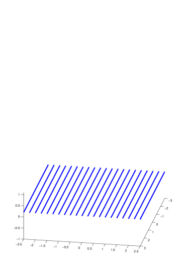
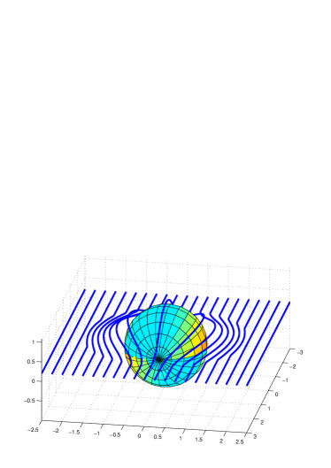
Figure 7: Left, light rays are shown in the Euclidian space $\mathbb{R}^{3}$ and right, the same light rays are shown when a cloaking device $(N,\widetilde{g})$ is located in the ball $B(0,1)$. The metamaterial in which the light rays travel is not shown; the sphere is the cloaking surface $\partial B(0,1)$. On left, the light rays correspond to geodesics on $(M_{1}\setminus\{0\},g)$ and on right, the geodesics on $(N_{1},\widetilde{g})$. The map $F_{1}$ maps the geodesics on $M_{1}$ (not passing through origin) to those of $N_{1}$.

The cloaking effect was justified in [93] on the level of the chain rule for $F_{1}$, and in the sequels [94, 27] on the level of rays and numerical simulations, on $N_{1}$. We will see below that studying the behavior of the waves on the entire space, including in the cloaked region $N_{2}$ and at the cloaking surface $\Sigma$, is crucial to fully understanding cloaking and its limitations.

A particular difficulty is that, due to the degeneracy of $\widetilde{\varepsilon}$ and $\widetilde{\mu}$, the weighted $L^{2}$ space defined by the energy norm

$$\|\widetilde{E}\|_{L^{2}(N,|\widetilde{g}|^{\frac{1}{2}}dx)}^{2}+\|\widetilde{H}\|_{L^{2}(N,|\widetilde{g}|^{\frac{1}{2}}dx)}^{2}=\int_{N}(\widetilde{\varepsilon}^{jk}\,\widetilde{E}_{j}\,\overline{\widetilde{E}_{k}}+\widetilde{\mu}^{jk}\,\widetilde{H}_{j}\,\overline{\widetilde{H}_{k}})\,dx$$ (44)

includes forms, which are not distributions, i.e., not in the dual of the vector fields having $C^{\infty}_{0}(N)$ coefficients. Indeed, this class contains the forms with the radial component behaving like $O((r-1)^{-\alpha})$ in the domain $r>1$, where $1<\alpha<3/2$. The meaning of the Helmholtz or Maxwell’s equations for such “waves” is problematic, and to treat cloaking rigorously, one should consider the boundary measurements (or scattering data) of finite energy waves which also satisfy Maxwell’s equations in some reasonable weak sense. Analysis of cloaking from this more rigorous point of view was carried out in [35], which forms the basis for much of the discussion here.

4.3 Cloaking for the Helmholtz equation

Let us start with the cases of scalar optics or acoustics, governed in the case of isotropic media by the Helmholtz equation (40). In order to work with anisotropic media, we convert this to the Helmholtz equation with respect to a Riemannian metric $g$. Working in dimensions $n\geq 3$, we take advantage of the one-to-one correspondence (28) between (positive definite) conductivities and Riemannian metrics $g$. Let us consider the Helmholtz equation

$$(\Delta_{g}+k^{2})u=\rho,$$ (45)

where $\Delta_{g}$ is the Laplace-Beltrami operator associated with the Euclidian metric $g_{ij}=\delta_{ij}$. Under a smooth diffeomorphism $F$, the metric $g$ pushes forward to a metric $\widetilde{g}=F_{*}g$, and then, for $u=\widetilde{u}\circ F$, we have

$$(\Delta_{g}+k^{2})u=\rho\iff(\Delta_{\widetilde{g}}+k^{2})\widetilde{u}=\widetilde{\rho},$$ (46)

where $\rho=\widetilde{\rho}\circ F$.

Next we consider the case when $F(x)$ is not a smooth diffeomorphism, but the one introduced by (32), if $x\in M_{1}\setminus\{0\}$ and identity, if $x\in M_{2}$.

Let $\widetilde{f}\in L^{2}(N,dx)$ be a function such that $\hbox{supp}\,(\widetilde{f})\cap\Sigma=\emptyset$. We now give the precise definition of a finite energy solution for the Helmholtz equation.

Definition 4.1

Let $g$ be the Euclidian metric on $M$ and $\widetilde{g}=F_{*}g$ be the singular metric on $N\setminus\Sigma$. A measurable function $\widetilde{u}$ on $N$ is a finite energy solution of the Dirichlet problem for the Helmholtz equation on $N$,

$$(\Delta_{\widetilde{g}}+k^{2})\widetilde{u}=\widetilde{f}\quad\hbox{on }N,$$ (47)

$$\widetilde{u}|_{\partial N}=\widetilde{h},$$

if

$$\widetilde{u}\in L^{2}(N,\,|\widetilde{g}|^{1/2}dx);$$ (48)

$$\widetilde{u}|_{N\setminus\Sigma}\in H^{1}_{loc}(N\setminus\Sigma,dx);$$ (49)

$$\int_{N\setminus\Sigma}|\widetilde{g}|^{1/2}\widetilde{g}^{ij}\partial_{i}\widetilde{u}\partial_{j}\widetilde{u}\,dx<\infty,$$ (50)

$$\widetilde{u}|_{\partial N}=\widetilde{h};$$

and, for all ${\widetilde{\psi}}\in C^{\infty}(N)\hbox{ with }{\widetilde{\psi}}|_{\partial N}=0$,

$$\int_{N}[-(D^{j}_{\widetilde{g}}\widetilde{u})\partial_{j}{\widetilde{\psi}}+k^{2}\widetilde{u}{\widetilde{\psi}}|\widetilde{g}|^{1/2}]dx=\int_{N}\widetilde{f}(x){\widetilde{\psi}}(x)|\widetilde{g}|^{1/2}dx$$ (51)

where $D^{j}_{\widetilde{g}}\widetilde{u}=|\widetilde{g}|^{1/2}\widetilde{g}^{ij}\partial_{i}u$ is defined as a Borel measure defining a distribution on $N$.

Note that the inhomogeneity $\widetilde{f}$ is allowed to have two components, $\widetilde{f}_{1}$ and $\widetilde{f}_{2}$, supported in the interiors of $N_{1},N_{2}$, resp. The latter corresponds to an active object being rendered undetectable within the cloaked region. On the other hand, the former corresponds to an active object embedded within the metamaterial cloak itself, whose position apparently shifts in a predictable manner according to the transformation $F_{1}$; this phenomenon, which also holds for both spherical and cylindrical cloaking for Maxwell’s equations, was later described and numerically modelled in the cylindrical setting, and termed the “mirage effect” [126].

Next we consider the relation between the finite energy solutions on $N$ and the solutions on $M$.

Theorem 4.2

([35]) Let $u=(u_{1},u_{2}):(M_{1}\setminus\{0\})\cup M_{2}\to\mathbb{R}$ and $\widetilde{u}:N\setminus\Sigma\to\mathbb{R}$ be measurable functions such that $u=\widetilde{u}\circ F$. Let $f=(f_{1},f_{2}):(M_{1}\setminus\{0\})\cup M_{2}\to\mathbb{R}$ and $\widetilde{f}:N\setminus\Sigma\to\mathbb{R}$ be $L^{2}$ functions, supported away from $0\in M_{1}$ and $\Sigma\subset N$ such that $f=\widetilde{f}\circ F$. At last, let $\widetilde{h}:\partial N\to\mathbb{R},\,h:\partial M_{1}\to\mathbb{R}$ be such that $h=\widetilde{h}\circ F_{1}$.

Then the following are equivalent:

1. The function $\widetilde{u}$, considered as a measurable function on $N$, is a finite energy solution to the Helmholtz equation (47) with inhomogeneity $\widetilde{f}$ and Dirichlet data $\widetilde{h}$ in the sense of Definition 4.1.

2. The function $u$ satisfies

   $$(\Delta_{g}+k^{2})u_{1}=f_{1}\quad\hbox{ on }M_{1},\quad u_{1}|_{\partial M_{1}}=h,$$ (52)

   and

   $$(\Delta_{g}+k^{2})u_{2}=f_{2}\quad\hbox{ on }M_{2},\quad g^{jk}\nu_{j}\partial_{k}u_{2}|_{\partial M_{2}}=b,$$ (53)

   with $b=0$. Here $u_{1}$ denotes the continuous extension of $u_{1}$ from $M_{1}\setminus\{0\}$ to $M_{1}$.

Moreover, if $u$ solves (52) and (53) with $b\not=0$, then the function $\widetilde{u}=u\circ F^{-1}:N\setminus\Sigma\to\mathbb{R}$, considered as a measurable function on $N$, is not a finite energy solution to the Helmholtz equation.

As mentioned in §1, and detailed in [39], this result also describes a structure which cloaks both passive objects and active sources for acoustic waves. Equivalent structures in the spherically symmetric case and with only cloaking of passive objects verified were considered later in [23, 29].

The idea of the proof of Thm. 4.2 is to consider $F_{1}$ and $F_{2}$ as coordinate transformations. As in formula (46), we see that if $u$ is a finite energy solution of the Helmholtz equation (47) in $N$ then $u_{1}=u\circ F_{1}$, defined in $M_{1}\setminus\{0\}$, satisfies the Helmholtz equation (52) on the set $M_{1}\setminus\{0\}$. Moreover, as the energy is invariant under a change of coordinates, one sees that $u|_{M_{1}\setminus\{0\}}$ is in the Sobolev space $H^{1}(M_{1}\setminus\{0\})$. Since the point $\{0\}$ has Hausdorff dimension less or equal the dimension of $\mathbb{R}^{3}$ minus two, the possible singularity of $u_{1}$ at zero is removable (see e.g., [60]), that is, $u_{1}$ has an extension to a function defined on the whole ball $M_{1}$ so that the Helmholtz equation (52) is satisfied on the whole ball.

Let us next discuss the appearance of the Neumann boundary condition in (53). Observe that in Def. 4.1 the Borel measure $D^{j}_{\widetilde{g}}v=|\widetilde{g}|^{1/2}\widetilde{g}^{ij}\partial_{i}v$ is absolutely continuous with respect to the Lebesgue measure for all functions $v\in C^{\infty}_{0}(N)$. We can approximate the finite energy solution $\widetilde{u}$ of equation (47) with source $\widetilde{f}$, supported away from $\Sigma$, by such functions. This yields that the measure of the cloaking surface satisfies $D^{j}_{\widetilde{g}}\widetilde{u}(\Sigma)=0$. Thus, using integration by parts, we see for arbitrary $\widetilde{\psi}\in C^{\infty}_{0}(N)$ that

$$0 = \lim_{\varepsilon\to 0+}\int_{B(0,1+\varepsilon)\setminus B(0,1-\varepsilon)}[(D^{j}_{\widetilde{g}}\widetilde{u})\partial_{j}{\widetilde{\psi}}-k^{2}\widetilde{u}{\widetilde{\psi}}|\widetilde{g}|^{1/2}]dx$$ (54)

$$= \lim_{\varepsilon\to 0+}\left(\int_{\partial B(0,1+\varepsilon)}-\int_{\partial B(0,1-\varepsilon)}\right)[\nu_{j}\,(|\widetilde{g}|^{1/2}\widetilde{g}^{ij}\partial_{i}\widetilde{u}]\,{\widetilde{\psi}}\,dS(x),$$

where $dS$ is the Euclidian surface area. Changing coordinates by $F_{1}^{-1}:\partial B(0,1+\varepsilon)\to\partial B(0,2\varepsilon)$ in the first integral in (54) and letting $\varepsilon\to 0$ in the second integral, we see that

$$0=\lim_{\varepsilon\to 0+}\int_{\partial B(0,2\varepsilon)}\frac{\partial u_{1}}{\partial\nu}\psi\,dS-\int_{\Sigma}\left.\frac{\partial\widetilde{u}}{\partial\nu}\right|_{\Sigma-}\widetilde{\psi}\,dS,$$ (55)

where $\psi=(F_{1})^{*}\widetilde{\psi}$ is a bounded function on $M_{1}$ and $u_{1}$ is the solution of (52) in $M_{1}$, hence smooth near $0$. Here $\left.\frac{\partial u}{\partial\nu}\right|_{\Sigma-}$ denotes the interior normal derivative. Thus, the first integral in (55) over the sphere of radius $2\varepsilon$ goes to zero as $\varepsilon\to 0$ yielding that the last integral must vanish. As $\widetilde{\psi}$ is arbitrary, this implies that $u$ satisfies the homogeneous boundary condition on the inside of the cloaking surface $\Sigma$. We point out that this Neumann boundary condition is a consequence of the fact that the coordinate transformation $F$ is singular on the cloaking surface $\Sigma$. See also [61] for the planar case.

4.4 Cloaking for Maxwell’s equations

In what follows, we treat Maxwell’s equations in non-conducting and lossless media, that is, for which the conductivity vanishes and the components of $\varepsilon,\mu$ are real valued. Although somewhat suspect (presently, metamaterials are quite lossy), these are standard assumptions in the physical literature. We point out that Ola, Päivärinta and Somersalo [91] have shown that cloaking is not possible for Maxwell’s equations with non-degenerate isotropic, sufficiently smooth, electromagnetic parameters.

We will use the invariant formulation of Maxwell’s equations. To this end, consider a smooth compact oriented connected Riemannian 3-manifold $M$, $\partial M\neq\emptyset$, with a metric $g$, that we call the background metric. Clearly, in physical applications we take $M\subset\mathbb{R}^{3}$ with $g$ being the Euclidean metric $g_{0}$. Time-harmonic Maxwell’s equations on the manifold $M$ are equations of the form

$${\rm curl}\,E(x)=ikB(x),$$ (56)

$${\rm curl}\,H(x)=-ikD(x)+J.$$ (57)

Here the electric field $E$ and the magnetic field $H$ are 1-forms and the electric flux $D$ and the magnetic flux $B$ are 2-forms, and curl is the standard exterior differential $d$. The external current $J$ is considered also as a 2-form. The above fields are related by the constitutive relations,

$$D(x)=\varepsilon(x)E(x),\quad B(x)=\mu(x)H(x),$$ (58)

where $\varepsilon$ and $\mu$ are linear maps from 1-forms to 2-forms. Thus, in local coordinates on $M$, we denote

$$E=E_{j}(x)dx^{j},\quad D=D^{1}(x)dx^{2}\wedge dx^{3}+D^{2}(x)dx^{3}\wedge dx^{1}+D^{3}(x)dx^{1}\wedge dx^{2},$$

$$H=H_{j}(x)dx^{j},\quad B=B^{1}(x)dx^{2}\wedge dx^{3}+B^{2}(x)dx^{3}\wedge dx^{1}+B^{3}(x)dx^{1}\wedge dx^{2}.$$

Using these notations, the constitutive relations take the form $D^{j}=\varepsilon^{jk}E_{k}$ and $B^{j}=\mu^{jk}H_{k}$.

Note, that in the case of a homogeneous Euclidian space, where $\varepsilon_{0}=1,\mu_{0}=1$, the operators $\varepsilon$ and $\mu$ correspond to the standard Hodge star operator $*:\Omega^{1}(\mathbb{R}^{3})\to\Omega^{2}(\mathbb{R}^{3})$ corresponding to the Euclidian metric $(g_{0})_{jk}=\delta_{jk}$. On an arbitrary manifold $(M,g)$ it is always possible to define the permittivity $\varepsilon$ and permeability $\mu$, to be the Hodge star operator corresponding to the metric $g$. Then, in local coordinates on $M$,

$$\varepsilon^{jk}=\mu^{jk}=|g|^{1/2}g^{jk}.$$ (59)

This type of electromagnetic material parameters, which has the same transformation law, under the change of coordinates, as the conductivity, was studied in [67].

To introduce the material parameters $\widetilde{\varepsilon}(x)$ and $\widetilde{\mu}(x)$ in the ball $N=B(0,2)\subset\mathbb{R}^{3}$ that make cloaking possible, we start with the singular map $F_{1}$ given by (32). We then introduce the Euclidean metric on $N_{2}$ and the metric $\widetilde{g}=F_{*}g$ in $N_{1}$. Finally, we define the singular permittivity and permeability in $N$ using the transformation rules (59) which lead to the formulae analogous to (36),

$$\widetilde{\varepsilon}^{jk}=\widetilde{\mu}^{jk}=\left\{\begin{array}[]{ll}|\widetilde{g}|^{1/2}\widetilde{g}^{jk}&\hbox{for }x\in N_{1},\\ \delta^{jk}&\hbox{for }x\in N_{2}.\end{array}\right.$$ (62)

Clearly that, as in the case of Helmholtz equations, these material parameters are singular on $\Sigma$.

We note that in $N_{2}$ one could define $\widetilde{\varepsilon}$ and $\widetilde{\mu}$ to be arbitrary smooth non-degenerate material parameters. For simplicity, we consider here only the homogeneous material in the cloaked region $N_{2}$.

4.5 Definition of solutions of Maxwell equations

In the rest of this section, $\varepsilon=1$ and $\mu=1$ on the manifold $M$ and $\widetilde{\varepsilon}$ and $\widetilde{\mu}$ are singular material parameter on $N$ defined in (62).

Since the material parameters $\widetilde{\varepsilon}$ and $\widetilde{\mu}$ are again singular at the cloaking surface $\Sigma$, we need a careful formulation of the notion of a solution.

Definition 4.3

We say that $(\widetilde{E},\widetilde{H})$ is a finite energy solution to Maxwell’s equations on $N$,

$$\nabla\times\widetilde{E}=ik\widetilde{\mu}(x)\widetilde{H},\quad\nabla\times\widetilde{H}=-ik\widetilde{\varepsilon}(x)\widetilde{E}+\widetilde{J}\quad\hbox{ on }N,$$ (63)

if $\widetilde{E}$, $\widetilde{H}$ are one-forms and $\widetilde{D}:=\widetilde{\varepsilon}\,\widetilde{E}$ and $\widetilde{B}:=\widetilde{\mu}\,\widetilde{H}$ two-forms in $N$ with $L^{1}(N,dx)$-coefficients satisfying

$$\|\widetilde{E}\|_{L^{2}(N,|\widetilde{g}|^{1/2}dV_{0}(x))}^{2}=\int_{N}\widetilde{\varepsilon}^{jk}\,\widetilde{E}_{j}\,\overline{\widetilde{E}_{k}}\,dV_{0}(x)<\infty,$$ (64)

$$\|\widetilde{H}\|_{L^{2}(N,|\widetilde{g}|^{1/2}dV_{0}(x))}^{2}=\int_{N}\widetilde{\mu}^{jk}\,\widetilde{H}_{j}\,\overline{\widetilde{H}_{k}}\,dV_{0}(x)<\infty;$$ (65)

where $dV_{0}$ is the standard Euclidean volume and

$$\int_{N}((\nabla\times\widetilde{h})\,\cdotp\widetilde{E}-ik\widetilde{h}\,\cdotp\widetilde{\mu}(x)\widetilde{H})\,dV_{0}(x)=0,$$ (66)

$$\int_{N}((\nabla\times\widetilde{e})\,\cdotp\widetilde{H}+\widetilde{e}\,\cdotp(ik\widetilde{\varepsilon}(x)\widetilde{E}-\widetilde{J}))\,dV_{0}(x)=0$$

for all 1-forms $\widetilde{e},\widetilde{h}$ on $N$ having in the Euclidian coordinates components in $C^{\infty}_{0}(N)$.

Above, the inner product “$\cdotp$” denotes the Euclidean inner product. We emphasize that in Def. 4.3 we assume that the components of the physical fields $\widetilde{E},\widetilde{H},\widetilde{B},$ and $\widetilde{D}$ are integrable functions. This in particular implies that the components of these fields are distributions. Note that the map $F_{*}$ does not map distributions on $M$ isomorphically to distributions on $N$. This is because $F^{*}:\phi\mapsto\phi\circ F$ does not map $C^{\infty}_{0}(N)$ to $C_{0}^{\infty}(M)$. Hence, on $M$ there are currents (i.e. sources) $J$, whose support contains the point zero that do not correspond to distributional sources $\widetilde{J}$ on $N$ for which $\widetilde{J}=F_{*}J$ in $N\setminus\Sigma$. Below we will show that in the case when a source $J$ is not supported on $N_{2}\cup\Sigma$, there exist solutions for Maxwell’s equations on $N$ with the corresponding source so that $\widetilde{J}=F_{*}J$ in $N\setminus\Sigma$. Also, we show that surprisingly, the finite energy solutions do not exist for generic currents $\widetilde{J}$. Roughly speaking, the fact that the map $F$ can not be extended to the whole $M$, so that it would map the differentiable structure on $M$ to that of $N$, seems to be the reason for this phenomena.

Below, we denote $M\setminus\{0\}=(M_{1}\setminus\{0\})\cup M_{2}$.

Theorem 4.4

([35]) Let $E$ and $H$ be 1-forms with measurable coefficients on $M\setminus\{0\}$ and $\widetilde{E}$ and $\widetilde{H}$ be 1-forms with measurable coefficients on $N\setminus\Sigma$ such that $\widetilde{E}=F_{*}E$, $\widetilde{H}=F_{*}H$. Let $J$ and $\widetilde{J}$ be 2-forms with smooth coefficients on $M\setminus\{0\}$ and $N\setminus\Sigma$, that are supported away from $\{0\}$ and $\Sigma$ such that $\widetilde{J}=F_{*}J$.

Then the following are equivalent:

1. The 1-forms $\widetilde{E}$ and $\widetilde{H}$ on $N$ satisfy Maxwell’s equations

   $$\nabla\times\widetilde{E}=ik\widetilde{\mu}(x)\widetilde{H},\quad\nabla\times\widetilde{H}=-ik\widetilde{\varepsilon}(x)\widetilde{E}+\widetilde{J}\quad\hbox{ on }N,$$ (67)

   $$\nu\times\widetilde{E}|_{\partial N}=f$$

   in the sense of Definition 4.3.

2. The forms $E$ and $H$ satisfy Maxwell’s equations on $M$,

   $$\nabla\times E=ik\mu(x)H,\quad\nabla\times H=-ik\varepsilon(x)E+J\quad\hbox{ on }M_{1},$$ (68)

   $$\nu\times E|_{\partial M_{1}}=f$$

   and

   $$\nabla\times E=ik\mu(x)H,\quad\nabla\times H=-ik\varepsilon(x)E+J\quad\hbox{ on }M_{2}$$ (69)

   with Cauchy data

   $$\nu\times E|_{\partial M_{2}}=b^{e},\quad\nu\times H|_{\partial M_{2}}=b^{h}$$ (70)

   that satisfies $b^{e}=b^{h}=0$.

Moreover, if $E$ and $H$ solve (68), (69), and (70) with non-zero $b^{e}$ or $b^{h}$, then the fields $\widetilde{E}$ and $\widetilde{H}$ are not solutions of Maxwell equations on $N$ in the sense of Definition 4.3.

Let us briefly discuss the proof of this theorem. In Euclidian space, with $\varepsilon=1$ and $\mu=1$, Maxwell’s equations (41) with $J=0$ and $k\not=0$ imply that the divergence of $D$ and $B$ fields are zero, or equivalently that

$$\nabla\,\cdotp(\varepsilon E)=0,\quad\nabla\,\cdotp(\mu H)=0.$$

Since $\varepsilon=1$ and $\mu=1$, we obtain using (41) and the basic formulae of calculus,

$$\Delta E=\sum_{j=1}^{3}\frac{\partial^{2}}{\partial x_{j}^{2}}E=\nabla(\nabla\,\cdotp E)-\nabla\times\nabla\times E=0-\nabla\times(ik\mu H)=-k^{2}E.$$

This implies the Helmholtz equation $(\Delta+k^{2})E=0$. Thus, removable singularity results similar to those used to prove Thm. 4.2 for the Helmholtz equation can be applied to Maxwell’s equations to show that equations (67) on $N$ imply Maxwell’s equations (68) first on $M_{1}\setminus\{0\}$ and then on all of $M_{1}$. Also, analogous computations to those presented after Thm. 4.2 for the finite energy solutions $(E,H)$ of Maxwell’s equations yield that the electric field $E$ has to satisfy the boundary condition $\nu\times E|_{\Sigma-}=0$ on the inside of the cloaking surface. As $E$ and $H$ are in symmetric roles, it follows that also the magnetic field has to satisfy $\nu\times H|_{\Sigma-}=0$. Summarizing, these considerations show that the finite energy solutions that are also solutions in the sense of distributions, have outside the cloaking surface a one-to-one correspondence to the solutions of Maxwell’s equations with the homogeneous, isotropic $\varepsilon_{0}$ and $\mu_{0}$ on $M_{1}$, but inside the cloaking region must satisfy hidden boundary conditions at $\Sigma^{-}$.

Thm. 4.4 can be interpreted by saying that the cloaking of active objects is difficult since, with non-zero currents present within the region to be cloaked, the idealized model leads to non-existence of finite energy solutions. The theorem says that a finite energy solution must satisfy the hidden boundary conditions

$$\nu\times\widetilde{E}=0,\quad\nu\times\widetilde{H}=0\quad\hbox{on }\partial N_{2}.$$ (71)

Unfortunately, these conditions, which correspond physically to the so-called perfect electrical conductor (PEC) and perfect magnetic conductor (PMC) conditions, simultaneously, constitute an overdetermined set of boundary conditions for Maxwell’s equations on $N_{2}$ (or, equivalently, on $M_{2}$). For cloaking passive objects, for which $J=0$, they can be satisfied by fields which are identically zero in the cloaked region, but for generic $J$, including ones arbitrarily close to 0, there is no solution. The perfect, ideal cloaking devices in practice can only be approximated with a medium whose material parameters approximate the degenerate parameters $\widetilde{\varepsilon}$ and $\widetilde{\mu}$. For instance, one can consider metamaterials built up using periodic structures whose effective material parameters approximate $\widetilde{\varepsilon}$ and $\widetilde{\mu}$. Thus the question of when the solutions exist in a reasonable sense is directly related to the question of which approximate cloaking devices can be built in practice. We note that if $E$ and $H$ solve (68), (69), and (70) with non-zero $b^{e}$ or $b^{h}$, then the fields $\widetilde{E}$ and $\widetilde{H}$ can be considered as solutions to a set of non-homogeneous Maxwell equations on $N$ in the sense of Definition 4.3.

$$\nabla\times\widetilde{E}=ik\widetilde{\mu}(x)\widetilde{H}+\widetilde{K}_{surf},\quad\nabla\times\widetilde{H}=-ik\widetilde{\varepsilon}(x)\widetilde{E}+\widetilde{J}+\widetilde{J}_{surf}\quad\hbox{ on }N,$$

where $\widetilde{K}_{surf}$ and $\widetilde{J}_{surf}$ are magnetic and electric surface currents supported on $\Sigma$. The appearance of these currents has been discussed in [35, 37, 124]. We note that there are many possible choices for the currents $\widetilde{J}_{surf}$ and $\widetilde{K}_{surf}$. If we include a PEC lining on $\Sigma$, that in physical terms means that we add a thin surface made of perfectly conducting material on $\Sigma$, the solution for the given boundary value $f$ is the one for which the magnetic boundary current vanish, $\widetilde{K}_{surf}=0$ and the electric boundary current $\widetilde{J}_{surf}$ is possibly non-zero. Introducing this lining on the cloaking surface $\Sigma$ turns out to be a remedy for the non-existence results, and we will see that the invisibility cloaking then be allowed to function as desired.

To define the boundary value problem corresponding to PEC lining, denote by $C^{\infty}_{\Sigma}(N)$ the space of functions $f:N\to\mathbb{R}$ such that $f|_{N_{1}}$ and $f|_{N_{2}}$ are $C^{\infty}$ smooth up to the boundary.

Definition 4.5

We say that $(\widetilde{E},\widetilde{H})$ is a finite energy solution to Maxwell’s equations on $N\setminus\Sigma$ with perfectly conducting cloaking surface,

$$\nabla\times\widetilde{E}=ik\widetilde{\mu}(x)\widetilde{H},\quad\nabla\times\widetilde{H}=-ik\widetilde{\varepsilon}(x)\widetilde{E}+\widetilde{J}\quad\hbox{ on }N\setminus\Sigma,$$ (72)

$$\nu\times E|_{\Sigma}=0$$

if $\widetilde{E}$, $\widetilde{H}$ are one-forms and $\widetilde{D}:=\widetilde{\varepsilon}\,\widetilde{E}$ and $\widetilde{B}:=\widetilde{\mu}\,\widetilde{H}$ two-forms in $N$ with $L^{1}(N,dx)$-coefficients satisfying conditions (64-65), and equations (66) hold for all 1-forms $\widetilde{e}$ and $\widetilde{h}$ on $N$ having in the Euclidian coordinates components in $C^{\infty}_{\Sigma}(N)$, vanishing near $\partial N$, and satisfing $\nu\times\widetilde{e}|_{\Sigma}=0$ from both sides of $\Sigma.$

With such lining of $\Sigma$, cloaking is possible with the following result, obtained similarly to Thm. 5 in [35] (cf. [35, Thm. 2 and 3]).

Theorem 4.6

Let $E$ and $H$ be 1-forms with measurable coefficients on $M\setminus\{0\}$ and $\widetilde{E}$ and $\widetilde{H}$ be 1-forms with measurable coefficients on $N\setminus\Sigma$ such that $\widetilde{E}=F_{*}E$, $\widetilde{H}=F_{*}H$. Let $J$ and $\widetilde{J}$ be 2-forms with smooth coefficients on $M\setminus\{0\}$ and $N\setminus\Sigma$, that are supported away from $\{0\}$ and $\Sigma$ such that $\widetilde{J}=F_{*}J$.

Then the following are equivalent:

1. The 1-forms $\widetilde{E}$ and $\widetilde{H}$ on $N$ satisfy Maxwell’s equations (72) in the sense of Definition 4.5.

2. The forms $E$ and $H$ satisfy Maxwell’s equations on $M$,

   $$\nabla\times E=ik\mu(x)H,\quad\nabla\times H=-ik\varepsilon(x)E+J\quad\hbox{ on }M_{1},$$ (73)

   and

   $$\nabla\times E=ik\mu(x)H,\quad\nabla\times H=-ik\varepsilon(x)E+J\quad\hbox{ on }M_{2},$$ (74)

   $$\nu\times E|_{\partial M_{2}}=0.$$

The above results show that if we are building an approximate cloaking device with metamaterials, effective constructions could be done in such a way that the material approximates a cloaking material with PEC (or PMC lining), which gives rise to the boundary condition on the inner part of $\Sigma$ of the form $\nu\times E|_{\partial M_{2}}=0$ (or $\nu\times H|_{\partial M_{2}}=0)$. Another physically relevant lining is the so-called SHS (soft-and-hard surface) [57, 58, 48, 77]. Mathematically, it corresponds to a boundary condition on the inner part of $\Sigma$ of the form $E(X)=H(X)=0$, where $X$ is a tangent vector field on $\Sigma$. It is particularly useful for the cloaking of a cylinder $\{(x_{1},x_{2},x_{3})\in\mathbb{R}^{3}:(x_{1},x_{2})\in D\}$, $D\subset\mathbb{R}^{3}$, when $X$ is the vector $\frac{\partial}{\partial\theta}$ in cylindrical coordinates, see [35], [37]. Further examples of mathematically possible boundary conditions on the inner part of $\Sigma$, for a different notion of solution, can be found in [119].

The importance of the SHS lining in the context of cylindrical cloaking is discussed in detail in [37]. In that case, adding a special physical surface on $\Sigma$ improves significantly the behavior of approximate cloaking devices; without this kind of lining the fields blow up. Thus we suggest that the engineers building cloaking devices should consider first what kind of cloak with well-defined solutions they would like to approximate. Indeed, building up a material where solutions behave nicely is probably easier than building a material with huge oscillations of the fields.

As an alternative, one can avoid the above difficulties by modifying the basic construction by using a double coating. Mathematically, this corresponds to using an $F=(F_{1},F_{2})$ with both $F_{1},F_{2}$ singular, which gives rise to a singular Riemannian metric which degenerates in the same way as one approaches $\Sigma$ from both sides. Physically, the double coating construction corresponds to surrounding both the inner and outer surfaces of $\Sigma$ with appropriately matched metamaterials, see [35] for details.

5 Electromagnetic wormholes

We describe in this section another application of transformation optics which consists in “blowing” up a curve rather than a point. In [36, 38] a blueprint is given for a device that would function as an invisible tunnel, allowing electromagnetic waves to propagate from one region to another, with only the ends of the tunnel being visible. Such a device, making solutions of Maxwell’s equations behave as if the topology of $\mathbb{R}^{3}$ has been changed to that $\mathbb{R}^{3}\#({\mathbb{S}}^{2}\times{\mathbb{S}}^{1})$, the connected sum of the Euclidian space $\mathbb{R}^{3}$ and the product manifold ${\mathbb{S}}^{2}\times{\mathbb{S}}^{1}$. The connected sum is somewhat analogous to an Einstein-Rosen wormhole [32] in general relativity, and so we refer to this construction as an electromagnetic wormhole.

We start by considering, as in Fig. 8, a 3-dimensional wormhole manifold, $M=M_{1}\cup M_{2}/\sim$, with components

$$M_{1}=\mathbb{R}^{3}\setminus(B(O,1)\cup B(P,1)),$$

$$M_{2}={\mathbb{S}}^{2}\times[0,1].$$

Here $\sim$ corresponds to a smooth identification, i.e., gluing, of the boundaries $\partial M_{1}$ and $\partial M_{2}$.

An optical device that acts as a wormhole for electromagnetic waves at a given frequency $k$ can be constructed by starting with a two-dimensional finite cylinder

$$T={\mathbb{S}}^{1}\times[0,L]\subset\mathbb{R}^{3},$$

taking its neighborhood $K=\{x\in\mathbb{R}^{3}:\ \hbox{dist}(x,T)\leq\rho\}$, where $\rho>0$ is small enough and defining $N=\mathbb{R}^{3}\setminus K$.

Figure 8: A two dimensional schematic figure of wormhole construction by gluing surfaces. Note that the components of the artificial wormhole construction are three dimensional.

Let us put the SHS lining on the surface $\partial K$, corresponding to the angular vector field $X=\partial_{\theta}$ in the cylindrical coordinates $(r,\theta,z)$ in $\mathbb{R}^{3}$, and cover $K$ with an invisibility cloak of the single coating type. This material has permittivity $\widetilde{\varepsilon}$ and permeability $\widetilde{\mu}$ described below, which are singular at $\partial K$. Finally, let

$$U=\{x:\ \hbox{dist}(x,K)>1\}\subset\mathbb{R}^{3}.$$

The set $U$ can be considered both as a subset of $N$, $U\subset N(\subset\mathbb{R}^{3})$ and of the introduced earlier abstract wormhole manifold $M$, $U\subset M_{1}$. Let us consider the electromagnetic measurements done in $U$, that is, measuring fields $E$ and $H$ satisfying a radiation condition that corresponds to an arbitrary current $J$ that is compactly supported in $U$. Then, as shown in [38], all electromagnetic measurements in $U\subset M$ and $U\subset N$ coincide; that is, waves on the wormhole device $(N,\widetilde{\varepsilon},\widetilde{\mu})$ in $\mathbb{R}^{3}$ behave as if they were propagating on the abstract wormhole manifold $M$.

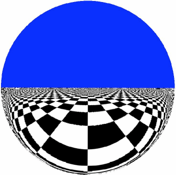
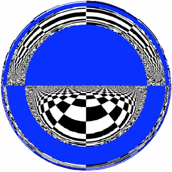
Figure 9: Ray tracing simulations of views through the bores of two wormholes. The distant ends are above an infinite chess board under a blue sky. On left, $L<<1$; on right, $L\approx 1$. Note that blue is used for clarity; the wormhole construction should be considered essentially monochromatic, for physical rather than mathematical reasons.

In Figures 3 and 9 we give ray-tracing simulations in and near the wormhole. The obstacle in Fig. 3 is $K$, and the metamaterial corresponding to $\widetilde{\varepsilon}$ and $\widetilde{\mu}$, through which the rays travel, is not shown.

We now give a more precise description of an electromagnetic wormhole. Let us start by making two holes in $\mathbb{R}^{3}$, say by removing the open unit ball $B_{1}=B(O,1)$, and also the open ball $B_{2}=B(P,1)$, where $P=(0,0,L)$ is a point on the $z$-axis with $L>3$, so that $\overline{B_{1}}\cap\overline{B_{2}}=\emptyset$. The region so obtained, $M_{1}=\mathbb{R}^{3}\setminus(B_{1}\cup B_{2})$, equipped with the standard Euclidian metric $g_{0}$ and a ”cut” $\gamma_{1}=\{(0,0,z):1\leq z\leq L-1\}$, is the first component $M_{1}$ of the wormhole manifold.

The second component of the wormhole manifold is a $3-$dimensional cylinder, $M_{2}=\mathbb{S}^{2}\times[0,1]$, with boundary $\partial M_{2}=(\mathbb{S}^{2}\times\{0\})\cup(\mathbb{S}^{2}\times\{1\}):=\mathbb{S}^{2}_{3}\cup\mathbb{S}^{2}_{4}$. We make a ”cut” $\gamma_{2}=\{NP\}\times[0,1]$, where $NP$ denotes an arbitrary point in $\mathbb{S}^{2}$, say the North Pole. We initially equip $M_{2}$ with the product metric, but several variations on this basic design are possible, having somewhat different possible applications which will be mentioned below.

Let us glue together the boundaries $\partial M_{1}$ and $\partial M_{2}$. The glueing is done so that we glue the point $(0,0,1)\in\partial B({\it O},1)$ with the point $NP\times\{0\}$ and the point $(0,0,L-1)\in\partial B(P,1)$ with the point $NP\times\{1\}$. Note that in this construction, $\gamma_{1}$ and $\gamma_{2}$ correspond to two nonhomotopic curves connecting $(0,0,1)\sim NP\times\{0\}$ to $(0,0,L-1)\sim NP\times\{1\}$. Moreover, $\gamma=\gamma_{1}\cup\gamma_{2}$ will be a closed curve on $M$.

Using cylindrical coordinates, $(r,\theta,z)\mapsto(r\cos\theta,r\sin\theta,z)$, let $N_{2}=\{(r,\theta,z):\ |r|<1,\ z\in[0,L]\}\cap N$ and $N_{1}=N\setminus N_{2}$; then consider singular transformations $F_{j}:M_{j}\setminus\gamma_{j}\longrightarrow\mathbb{R}^{3},\ j=1,2$, whose images are $N_{1},N_{2}$, resp., see [38] for details. For instance, the map $F_{1}$ can be chosen so that it keeps the $\theta$-coordinate the same and maps $(z,r)$ coordinates by $f_{1}:(z,r)\to(z^{\prime},r^{\prime})$. In the Fig. 10 the map $f_{1}$ is visualized.

Together the maps $F_{1}$ and $F_{2}$ define a diffeomorphism $F:M\setminus\gamma\to N$, that blows up near $\gamma$. We define the material parameters $\widetilde{\varepsilon}$ and $\widetilde{\mu}$ on $N$ by setting $\widetilde{\varepsilon}=F_{*}\varepsilon$ and $\widetilde{\mu}=F_{*}\mu$. These material parameters (having freedom in choosing the map $F$) give blueprints for how a wormhole device could be constructed in the physical space $\mathbb{R}^{3}$.

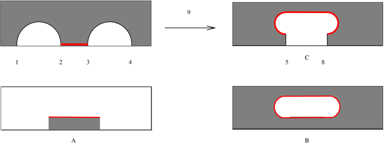
Figure 10: Above: A schematic figure of $f_{1}$, representing $F_{1}$, in the $(z,r)$ plane. Its image $P$ corresponds to $N_{1}$ in $(z,r)$ coordinates. Below: The sets $Q$ and $R$ correspond to $N_{2}$ and $N$. In the figure, $R=Q\cup P$ which corresponds to $N=N_{1}\cup N_{2}$ in $\mathbb{R}^{3}$.

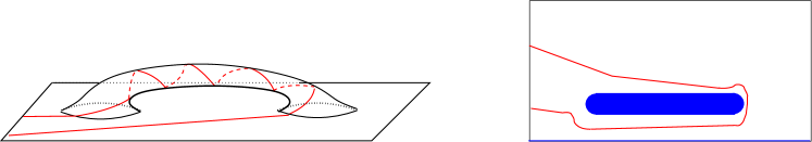
Figure 11: Schematic figure. Left: Some rays enter the wormhole and come out from the other end so that they return near where the ray entered to the wormhole. Right: The corresponding ray in the complement $N$ of the obstacle $K$ shown in the $(z,r)$ coordinates. Note that there are also closed light rays.

Possible applications of electromagnetic wormholes (with varying degrees of likelihood of realization!), when the metamaterials technology has sufficiently progressed, include invisible optical cables, 3D video displays, scopes for MRI-assisted medical procedures, and beam collimation. For the last two, one needs to modify the design by changing the metric $g_{2}$ on $M_{2}=\mathbb{S}^{2}\times[0,1]$. By flattening the metric on $\mathbb{S}^{2}$ so that the antipodal point $SP$ (the south pole) to $NP$ has a neighborhood on which the metric is Euclidian, the axis of the tunnel $N_{2}$ will have a tubular neighborhood on which $\varepsilon,\mu$ are constant isotropic and hence can be allowed to be empty space, allowing for passage of instruments. On the other hand, if we use a warped product metric on $M_{2}$, corresponding to $\mathbb{S}^{2}\times\{z\}$ having the metric of the sphere of radius $r(z)$ for an appropriately chosen function $r:[0,1]\longrightarrow\mathbb{R}_{+}$, then only rays that travel through $N_{2}$ almost parallel to the axis can pass all the way through, with others being returned to the end from which they entered.

Remark 5.1

Along similar lines, we can produce another interesting class of devices, made possible with the use of metamaterials, which behave as if the topology of $\mathbb{R}^{3}$ is altered. Let $M_{1}=\mathbb{R}^{3}\setminus B(0,1)$ endowed with the Euclidian metric $g$ and $M_{2}$ be a copy of $M_{1}$. Let $M$ be the manifold obtained by glueing the boundaries $\partial M_{1}$ and $\partial M_{2}$ together. Then $M$ can be considered as a $C^{\infty}$ smooth manifold with Lipschitz smooth metric. Let $N_{1}=M_{2}$ and $F_{1}:M_{1}\to N_{1}$ be the identity map, $N_{2}=B(0,1)\setminus\overline{B}(0,\rho)$ with $\rho\geq 0$, and finally $N=\mathbb{R}^{3}\setminus\overline{B}(0,\rho)$. Let $F_{2}:M_{2}\to N_{2}$ be the map $F_{2}(x)=(\rho+(1-\rho)|x|^{-1})|x|^{-1}x$. Together the maps $F_{1}$ and $F_{2}$ define a map that can be extended to a Lipschitz smooth diffeomorphism $F:M\to N$. As before, we define on $N$ the metric $\widetilde{g}=F_{*}g$, and the permittivity $\widetilde{\varepsilon}$ and permeability $\widetilde{\mu}$ according to formula (62). As $N=\mathbb{R}^{3}\#\mathbb{R}^{3}$, we can consider the $(N,\widetilde{\varepsilon},\widetilde{\mu})$ as a parallel universe device on which the electromagnetic waves on $\mathbb{R}^{3}\#\mathbb{R}^{3}$ can be simulated. It is particularly interesting to consider the high frequency case when the ray-tracing leads to physically interesting considerations. Light rays correspond to the locally shortest curves on $N$, so all rays emanating from $N_{1}$ that do not hit $\partial N_{1}$ tangentially then enter $N_{2}$. Thus the light rays in $N_{1}$ that hit $\partial N_{1}$ non-tangentially change the sheet $N_{1}$ to $N_{2}$. From the point of view of an observer in $N_{1}$, the rays are absorbed by the device. Thus on the level of ray-tracing the device is a perfectly black body, or a perfect absorber. Similarly analyzing the quasi-classical solutions, the energy, corresponding to the non-tangential directions is absorbed, up to the first order of magnitude, by the device. Other, metamaterial-based constructions of a perfect absorber have been considered in [68]. We note that in our considerations the energy is not in reality absorbed as there is no dissipation in the device, and thus the energy is in fact trapped inside the device, which naturally causes difficulties in practical implementation. On the level of the ray tracing similar considerations using multiple sheets have been considered before in [76].

6 A general framework:
singular transformation optics

Having seen how cloaking based on blowing up a point or blowing up a line can be rigorously analyzed, we now want to explore how more general optical devices can be described using the transformation rules satisfied by $n,(\rho,\lambda),\varepsilon$ and $\mu$. This point of view has been advocated by J. Pendry and his collaborators, and given the name transformation optics [116]. As discussed earlier, under a nonsingular changes of variables $F$, there is a one-to-one correspondence between solutions $\widetilde{u}$ of the relevant equations for the transformed medium and solutions $u=\widetilde{u}\circ F$ of the original medium. However, when $F$ is singular at some points, as is the case for cloaking and the wormhole, we have shown how greater care needs to be taken, not just for the sake of mathematical rigour, but to improve the cloaking effect for more physically realistic approximations to the ideal material parameters. Cloaking and the wormhole can be considered as merely starting points for what might be termed singular transformation optics, which, combined with the rapidly developing technology of metamaterials, opens up entirely new possibilities for designing devices having novel effects on acoustic or electromagnetic wave propagation. Other singular transformation designs in 2D that rotate waves within the cloak [21], concentrate waves [96] or act as beam splitters [97] have been proposed. Analogies with phenomena in general relativity have been proposed in [74] as a source of inspiration for designs.

We formulate a general approach to the precise description of the ideal material parameters in a singular transformation optics device, $N\subset\mathbb{R}^{3}$, and state a “metatheorem”, analogous to the results we have seen above, which should, in considerable generality, give an exact description of the electromagnetic waves propagating through such a device. However, we wish to stress that, as for cloaking [35] and the wormhole [36, 38], actually proving this “result” in particular cases of interest, and determining the hidden boundary conditions, may be decidedly nontrivial.

A general framework for considering ideal mathematical descriptions of such designs is as follows: Define a singular transformation optics (STO) design as a triplet $({\mathcal{M}},{\mathcal{N}},{\mathcal{F}})$, consisting of:

(i)  An STO manifold, ${\mathcal{M}}=(M,g,\gamma)$, where $M=(M_{1},\dots,M_{k})$, the disjoint union of $n$-dimensional Riemannian manifolds $(M_{j},g_{j})$, with or without boundary, and (possibly empty) submanifolds $\gamma_{j}\subset\hbox{int }M_{j}$, with $\dim\gamma_{j}\leq n-2$;

(ii)  An STO device, ${\mathcal{N}}=(N,\Sigma)$, where $N=\bigcup_{j=1}^{k}N_{j}\subset\mathbb{R}^{n}$ and $\Sigma=\bigcup_{j=1}^{k}\Sigma_{j}$, with $\Sigma_{j}$ a (possibly empty) hypersurface in $N_{j}$; and

(iii)  A singular transformation ${\mathcal{F}}=(F_{1},\dots,F_{k})$, with each $F_{j}:M_{j}\setminus\gamma_{j}\longrightarrow N_{j}\setminus\Sigma_{j}$ a diffeomorphism.

Note that $N$ is then equipped with a singular Riemannian metric $\widetilde{g}$, with $\widetilde{g}|_{N_{j}}=(F_{j})_{*}(g_{j})$, in general degenerate on $\Sigma_{j}$. Reasonable conditions need to be placed on the Jacobians $DF_{j}$ as one approached $\gamma_{j}$ so that the $\widetilde{g}_{j}$ have the appropriate degeneracy, cf. [45,  Thm.3].

In the context of the conductivity or Helmholtz equations, we can then compare solutions $u$ on ${\mathcal{M}}$ and $\widetilde{u}$ on ${\mathcal{N}}$, while for Maxwell we can compare fields $(E,H)$ on ${\mathcal{M}}$ (with $\varepsilon$ and $\mu$ being the Hodge-star operators corresponding to the metric $g$) and $(\widetilde{E},\widetilde{H})$ on ${\mathcal{N}}$. For simplicity, below we refer to the fields as just $u$.

Principle of Singular Transformation Optics, or “A Metatheorem about Metamaterials”: If $({\mathcal{M}},{\mathcal{N}},{\mathcal{F}})$ is an STO triplet, there is a 1-1 correspondence, given by $u=\widetilde{u}\circ{\mathcal{F}}$, i.e., $u|_{M_{j}}=(\widetilde{u}|_{N_{j}})\circ F_{j}$, between finite energy solutions $\widetilde{u}$ to the equation(s) on ${\mathcal{N}}$, with source terms $\widetilde{f}$ supported on ${\mathcal{N}}\setminus\Sigma$, and finite energy solutions $u$ on ${\mathcal{M}}$, with source terms $f=\widetilde{f}\circ{\mathcal{F}}$, satisfying certain “hidden” boundary conditions on $\partial M=\bigcup_{j=1}^{k}\,\partial M_{j}$.

7 Isotropic Transformation Optics

The design of transformation optics (TO) devices, based on the transformation rule (25), invariably leads to anisotropic material parameters. Furthermore, in singular TO designs, such as cloaks, field rotators [21], wormholes [36, 38], beam-splitters [97], or any of those arising from the considerations of the previous section, the material parameters are singular, with one or more eigenvalues going to 0 or $\infty$ at some points.

While raising interesting mathematical issues, such singular, anisotropic parameters are difficult to physically implement. The area of metamaterials is developing rapidly, but fabrication of highly anisotropic and (nearly) singular materials at frequencies of interest will clearly remain a challenge for some time. Yet another constraint on the realization of theoretically perfect ( or ideal in the physics nomenclature) TO designs is discretization: the metamaterial cells have positive diameter and any physical construction can represent at best a discrete sampling of the ideal parameters.

There is a way around these difficulties. At the price of losing the theoretically perfect effect on wave propagation that ideal TO designs provide, one can gain the decided advantages of being able to use discrete arrays of metamaterial cells with isotropic and nonsingular material parameters. The procedure used in going from the anisotropic, singular ideal parameters to the isotropic, nonsingular, discretized parameters involves techniques from the analysis of variational problems, homogenization and spectral theory. We refer to the resulting designs as arising from isotropic transformation optics. How this is carried out is sketched below in the context of cloaking; more details and applications can be found in [40, 41, 42].

The initial step is to truncate ideal cloaking material parameters, yielding a nonsingular, but still anisotropic, approximate cloak; similar constructions have been used previously in the analysis of cloaking [98, 37, 62, 24]. This approximate cloak is then itself approximated by nonsingular, isotropic parameters. The first approximation is justified using the notions of $\Gamma$- and $G$-convergence from variational analysis [8, 30], while the second uses more recent ideas from [2, 3, 26].

We start with the ideal spherical cloak for the acoustic wave equation. For technical reasons, we modify slightly the cloaking conductivity (36) by setting it equal to $2\delta^{jk}$ on $B(0,1)$, and relabel it as $\sigma$ for simplicity. Recall that $\sigma$ corresponds to a singular Riemannian metric $g_{jk}$ that is related to $\sigma^{ij}$ by

$$\sigma^{ij}(x)=|g(x)|^{1/2}g^{ij}(x),\quad|g|=\left(\hbox{det}[\sigma^{ij}]\right)^{2}$$ (75)

where $[g^{jk}(x)]$ is the inverse matrix of $[g_{jk}(x)]$ and $|g(x)|=\hbox{det}[g_{jk}(x)]$. The resulting Helmholtz equation, with a source term $p$,

$$\sum_{j,k=1}^{3}|g(x)|^{-1/2}\frac{\partial}{\partial x^{j}}(|g(x)|^{1/2}g^{jk}(x)\frac{\partial}{\partial x^{k}}u)+\omega^{2}u=p\quad\hbox{on }N,$$ (76)

$$u|_{\partial N}=f,$$

can then be reinterpreted by thinking of $\sigma$ as a mass tensor (which indeed has the same transformation law as conductivity under coordinate diffeomorphisms ) and $|g|^{\frac{1}{2}}$ as a bulk modulus parameter; (76) then becomes an acoustic wave equation at frequency $\omega$ with the new source $p|g|^{1/2}$,

$$\left(\nabla\cdotp\sigma\nabla+\omega^{2}|g|^{\frac{1}{2}}\right)u=p(x)|g|^{\frac{1}{2}}\quad\hbox{on }N,$$ (77)

$$u|_{\partial N}=f.$$

This is the form of the acoustic wave equation considered in [23, 29, 39]. (See also [28] for $d=2$, and [89] for cloaking with both mass and bulk modulus anisotropic.) To consider equation (77) rigorously, we assume that the source $p$ is supported away from the surface $\Sigma$. Then the finite energy solutions $u$ of equation (77) are defined analogously to Def. 4.1. Note that the function $|g|^{1/2}$ appearing in (77) is bounded from above.

Now truncate this ideal acoustic cloak: for each $1<R<2$, let $\rho=2(R-1)$ and define $F_{R}:\mathbb{R}^{3}\setminus B(0,\rho)\to\mathbb{R}^{3}\setminus B(0,R)$ by

$$x:=F_{R}(y)=\left\{\begin{array}[]{cl}y,&\hbox{for }|y|>2,\\ \left(1+\frac{|y|}{2}\right)\frac{y}{|y|},&\hbox{for }\rho<|y|\leq 2.\end{array}\right.$$

We define the corresponding approximate conductivity, $\sigma_{R}$ as

$$\sigma^{jk}_{R}(x)=\left\{\begin{array}[]{cl }\sigma^{jk}(x)&\hbox{for }|x|>R,\\ 2\delta^{jk},&\hbox{for }|x|\leq R,\end{array}\right.$$ (81)

where $\sigma^{jk}$ is the same as in the first formula in (36) or, in spherical coordinates, (37). Note that then $\sigma^{jk}(x)=\left(\left(F_{R}\right)_{*}\sigma_{0}\right)^{jk}(x)$ for $|x|>R$, where $\sigma_{0}\equiv 1$ is the homogeneous, isotropic mass density tensor. Observe that, for each $R>1$, $\sigma_{R}$ is nonsingular, i.e., is bounded from above and below, but with the lower bound going to $0$ as $R\searrow 1$. Now define

$$g_{R}(x)=\hbox{det}\,(\sigma_{R}(x))^{2}=\left\{\begin{array}[]{cl}64|x|^{-4}(|x|-1)^{4}&\hbox{for }R<|x|<2,\\ 64,&\hbox{for }|x|\leq R,\end{array}\right.$$ (84)

cf. (75). Similar to (77), consider the solutions of

$$(\nabla\cdotp\sigma_{R}\nabla+\omega^{2}g_{R}^{1/2})u_{R} = g_{R}^{1/2}p\quad\hbox{in }N$$ (85)

$$u_{R}|_{\partial N} = f.$$

As in Thm. 4.2, by considering $F_{R}$ as a transformations of coordinates one sees that

$$u_{R}(x)=\left\{\begin{array}[]{cl}v_{R}^{+}(F_{R}^{-1}(x)),&\hbox{for }R<|x|<2,\\ v_{R}^{-}(x),&\hbox{for }|y|\leq R,\end{array}\right.$$

with $v_{R}^{\pm}$ satisfying

$$(\Delta+\omega^{2})v_{R}^{+}(y) = p(F_{R}(y))\quad\hbox{in }\rho<|y|<2,$$

$$v_{R}^{+}|_{\partial B(0,2)} = f,$$

and

$$(\nabla^{2}+4\omega^{2})v_{R}^{-}(y) = 4p(y),\quad\hbox{in }|y|<R.$$ (87)

Since $\sigma_{R}$ and $g_{R}$ are nonsingular everywhere, we have the standard transmission conditions on $\Sigma_{R}:=\{x:\ |x|=R\}$,

$$u_{R}|_{\Sigma_{R}+}=u_{R}|_{\Sigma_{R}-},$$ (88)

$$e_{r}\cdotp\sigma_{R}\nabla u_{R}|_{\Sigma_{R}+}=e_{r}\cdotp\sigma_{R}\nabla u_{R}|_{\Sigma_{R}-},$$ (89)

where $e_{r}$ is the radial unit vector and $\pm$ indicates when the trace on $\Sigma_{R}$ is computed as the limit $r\to R^{\pm}$.

The resulting solutions, say for either no source, or for $p$ supported at the origin, can be analyzed using spherical harmonics, and one can show that the waves $v$ for the ideal cloak are the limits of the waves for the approximate cloaks, with the Neumann boundary condition in (53) for the ideal cloak emerging from the behavior of the waves $v_{R}^{\pm}$ for the truncated cloaks. This can be seen using spherical coordinates and observing that the trace of the radial component of conductivity from outside, $\sigma_{R}^{rr}|_{\Sigma_{R}+}$, goes to zero as $R\to 1$ but the trace $\sigma_{R}^{rr}|_{\Sigma_{R}+}$ from inside stays bounded from below. Using this, we can see that the transmission condition (89) explains the appearance of the Neumann boundary condition on the inside of the cloaking surface.

To consider general conductivities, we recall that for a conductivity $\gamma^{jk}(x)$ that is bounded both from above and below, the solution of the boundary value problem (22) in $N$ is the unique minimizer of the quadratic form

$${\mathcal{Q}}_{\gamma}(v)=\int_{N}\gamma\nabla v\,\cdotp\nabla v\,dx$$ (90)

over the functions $v\in H^{1}(N)$ satisfying the boundary condition $v|_{\partial N}=f$.

We use the above to consider the truncated conductivities $\sigma_{R}$. Note that at each point $x\in N$ the non-negative matrix $\sigma_{R}(x)$ is a decreasing function of $R$. Thus the quadratic forms $v\mapsto{\mathcal{Q}}_{\sigma_{R}}(v)$ are pointwise decreasing. As the minimizer $v$ of the quadratic form ${\mathcal{Q}}_{\sigma_{R}}(v)+\langle h,v\rangle_{L^{2}}$ with the condition $v|_{\partial N}=f$ is the solution of the equation

$$\nabla\cdotp\sigma_{R}\nabla v=h,\quad v|_{\partial N}=f,$$

we can use methods from variational analysis, in particular $\Gamma$-convergence (see, e.g., [30]) to consider solutions of equation (85). Using that, it is possible to show that the solutions $u_{R}$ of the approximate equations (85) converge to the solution $u$ of (77) for the general sources $p$ not supported on $\Sigma$ in the case when $\omega^{2}$ is not an eigenvalue of the equation (77).

Next, we approximate the nonsingular but anisotropic conductivity $\sigma_{R}$ with isotropic tensors. One can show that there exist nonsingular, isotropic conductivities $\gamma_{n}$ such that the solutions of

$$\left(g_{R}(x)^{-1/2}\nabla\cdotp\gamma_{n}(x)\nabla+\omega^{2}\right)u_{n}=p\quad\hbox{on }N,$$ (91)

$$u_{n}|_{\partial N}=f,$$

tend to the solution of (85) as $n\to\infty$. This is obtained by considering isotropic conductivities $\gamma_{n}(x)=h_{n}(|x|)$ depending only on radial variable $r=|x|$, where $h_{n}$ oscillates between large and small values. Physically, this corresponds to layered spherical shells having high and low conductivities. As the oscillation of $h_{n}$ increases, these spherical shells approximate an anisotropic medium where the conductivity has much lower value in the radial direction than in the angular variables. Roughly speaking, currents can easily flow in the angular directions on the highly conducting spherical shells, but the currents flowing in the radial direction must cross both the low and high conductivity shells. Rigorous analysis based on homogenization theory [2, 26] is used for $\omega^{2}\in\mathbb{R}_{-}$, and one can see that, with appropriately chosen isotropic conductivities $\gamma_{n}$, the solutions $u_{n}$ converge to the limit $u_{R}$. These considerations can be extended to all $\omega^{2}\in{\mathbb{C}}\setminus{\it D}$, where ${\it D}\subset\mathbb{R}_{-}$ is a discrete set, by spectral-theoretic methods, [55]. More details can be found in [40, 42].

Summarizing, considering equations (91) with appropriately chosen smooth isotropic conductivities $\gamma_{n}$ and bulk moduli $g_{R}$ and letting $n\to\infty$ with $R=R(n)\to 1$, we obtain Helmholtz equations with isotropic and non-singular mass and bulk modulus, whose solutions converge to the solution of the ideal invisibility cloak (77).

A particularly interesting application of the above construction is to quantum mechanics. Zhang, et al. [125] described an anisotropic mass tensor $\widehat{m}$ and a potential $V$ which together act as a cloak for matter waves, i.e., solutions of the corresponding anisotropic Schrödinger equation. This ideal quantum cloak is the result of applying the same singular transform $F$ as used for conductivity, Helmholtz and Maxwell, and applying it to the Schrödinger equation with mass tensor $\widehat{m}_{0}=\delta^{jk},\,V_{0}\equiv 0$. Due to the anisotropy of $\widehat{m}$, and the singularity of both $\widehat{m}$ and $V$, physical realization would be quite challenging. However, using the approximate acoustic cloak, one can describe an approximate quantum cloak that should be much easier to physically realize. An analogue of the reduction (14), (15) of the isotropic conductivity equation to a Schrödinger equation can be carried out for the acoustic equation. Letting $E=\omega^{2}$, $\psi_{n}(x)=\gamma_{n}^{1/2}(x)u_{n}(x)$, and

$$V_{n}^{E}(x):\,=\gamma_{n}^{-1/2}\nabla^{2}\gamma_{n}^{1/2}(x)-E\gamma_{n}^{-1}g_{n}^{1/2}+E,$$ (92)

one computes that $\psi_{n}$ satisfies the Schrödinger equation

$$(-\Delta+V_{n}^{E})\psi_{n}=E\psi_{n}\quad\hbox{in }\,\,N.$$

Furthermore, the family $\{V_{n}^{E}\}$ acts an approximate cloak at energy $E$:

Theorem 7.1

Approximate quantum cloaking. Let $W$ be a potential $W\in L^{\infty}(B(0,1))$, and $E\in\mathbb{R}$ not be a Dirichlet eigenvalue of $-\Delta$ on $N=B(0,2)$, nor a Neumann eigenvalue of $-\Delta+W$ on $B(0,1)$. The DN operators at $\partial N$ for the Schrödinger operators corresponding to the potentials $W+V_{n}^{E}$ converge to the DN operator corresponding to free space, that is,

$$\lim_{n\to\infty}\Lambda_{W+V_{n}^{E}}(E)f=\Lambda_{0}(E)f$$

in $L^{2}(\partial N)$ for any smooth $f$ on $\partial N$.

The convergence of the DN operators also implies convergence of the scattering amplitudes [12]: $\lim_{n\to\infty}a_{W+V_{n}^{E}}(E,\theta^{\prime},\theta)=a_{0}(E,\theta^{\prime},\theta)$.

(Note that this is not a consequence of standard results from perturbation theory, since the $V_{n}^{E}$ do not tend to $0$ as $n\to\infty$. Rather, as $n\to\infty$, the $V_{n}^{E}$ become highly oscillatory near $\Sigma$ and $\sup_{x}|V_{n}^{E}(x)|\to\infty$ as $n\to\infty$.)

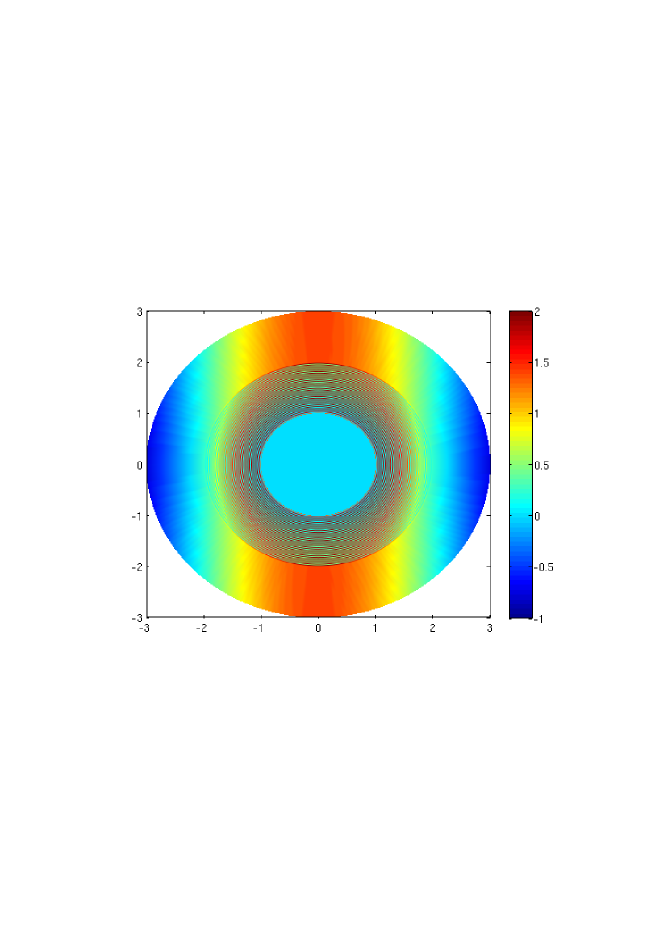
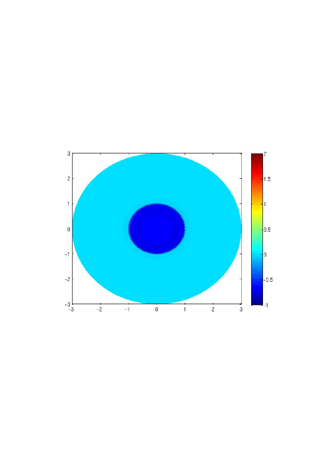
Figure 12: Left: $E$ not a Neumann eigenvalue; approximate quantum cloak. Matter wave passes almost unaltered. Right: $E$ a Neumann eigenvalue; potential supports almost trapped state.

On the other hand, when $E$ is a Neumann eigenvalue of $-\Delta+W$ on $B(0,1)$, then $V^{E}_{n}$ supports almost trapped states, which correspond to matter waves (i.e., quantum mechanical particles) which reside in $B(0,1)$ with high probability. See Fig. 12 and [41] for more details and applications.

Remark 7.2

Parameter distribution similar to (81) have been studied in the physics literature in the context of realistically achievable layouts of metamaterials approximating an ideal cloak. Using other, apparently only slightly different designs, one obtains in the limit other cloaking devices with enforced boundary conditions on the inside of $\Sigma$; see [40], where approximate cloaks are specified which give rise instead to the Robin boundary condition.

8 Further developments and open problems

The literature on metamaterials, cloaking, and transformation optics is growing rapidly . We briefly describe here only a few recent developments and remaining challenges. See [75] for a variety of perspectives.

(a)  Although the first description [44, 45] of the cloaking phenomenon was in the context of electrostatics, no proposals of electrostatic metamaterials that might be used to physically implement these examples have been made to date. A proposal for metamaterials suitable for magnetostatics (cloaking for which is of course mathematically identical to electrostatics), and magnetism at very low frequencies, is in [120]. Since [99], there has been a push to obtain cloaking at higher frequencies, with the visual part of the electromagnetic spectrum an obvious goal. Progress has been reported in [17, 104, 78, 102]. However, broadband visual cloaking seems at this point to be far off. It should also be pointed out that serious skepticism concerning the practical advantages of transformation optics based cloaking over earlier techniques for reducing scattering has been expressed [59].

(b)  Other boundary conditions at the cloaking surface, analyzed in the time domain, based on Von Neumann’s theory of self-adjoint extensions and using a different notion of solution than that considered here, have been studied in [117, 118, 119]. See also [121].

(c)  For simplicity, in cloaking we have mainly considered singular transformations which are affine linear in $r$. (See, however, Thm.  3.2.) In situations where the measurements are made further from cloaked object, [18] introduced, for spherical cloaking, transformations nonlinear in the radial variable in order to give better impedance matching with the surrounding media, and this was further explored for cylindrical cloaking in [122].

(d)  Effective medium theory for metamaterials is in its early development, and seems to be particularly difficult for materials assembled from periodic or almost-periodic arrays of small cells whose properties are based on resonance effects. A physical (although mathematically nonrigorous) analysis of this kind of media is in [103], which makes implicit assumptions about the smoothness of the fields which are violated when the fields experience the blow up demonstrated in [98, 37]. Some recent work on homogenization in this context is in [63]. However, further efforts in this directions are needed.

(e)  Existing theories of cloaking deal predominantly with non-relativistic media; see, however, [74]. It seems that developing a theory compatible with the relativistic framework would be important. Similarly, transformation optics in the context of nonlinear media seems likely to become significant as metamaterial technology develops.

(f)  At the cloaking surface $\Sigma$ the cloaking metric $\widetilde{g}$ on $N_{1}$ has a conical singularity in the sense of geometric scattering theory. It would be interesting to understand the relationship between cloaking and other transformation optics constructions on the one hand and geometric scattering on the other.

References

- [1] M. Ablowitz, D. Bar Yaacov and A. Fokas, On the inverse scattering transform for the Kadomtsev-Petviashvili equation, Studies Appl. Math. 69 (1983), 135–143.
- [2] G. Allaire: Homogenization and two-scale convergence, SIAM J. Math. Anal. 23 (1992), 1482-1518.
- [3] G. Allaire and A. Damlamian and U. Hornung, Two-scale convergence on periodic surfaces and applications, In A. Bourgeat, C. Carasso, S. Luckhaus and A. Mikelic (eds.), Mathematical Modelling of Flow through Porous Media, 15-25, Singapore, World Scientific, 1995.
- [4] A. Alu and N. Engheta, Achieving transparency with plasmonic and metamaterial coatings, Phys. Rev. E, 72, 016623 (2005)
- [5] K. Astala and L. Päivärinta: Calderón’s inverse conductivity problem in the plane. Annals of Math. 163 (2006), 265-299.
- [6] K. Astala, M. Lassas, and L. Päiväirinta, Calderón’s inverse problem for anisotropic conductivity in the plane, Comm. Partial Diff. Eqns. 30 (2005), 207–224.
- [7] K. Astala, M. Lassas, and L. Päivärinta, Limits of visibility and invisibility for Calderón’s inverse problem in the plane, in preparation.
- [8] H. Attouch, Variational convergence for functions and operators, Appl. Math. Series, Pitman, Boston, 1984. xiv+423 pp.
- [9] R. Beals and R. Coifman, Scattering, spectral transformations and nonlinear evolution equations. II, Goulaouic-Meyer-Schwartz Seminar, 1981/1982, Exp. No. XXI, (1982).
- [10] R. Beals and R. Coifman, Multidimensional inverse scatterings and nonlinear partial differential equations, in Pseudodifferential operators and applications (Notre Dame, Ind., 1984), 45–70, Proc. Sympos. Pure Math.,43, Amer. Math. Soc., Providence, RI, 1985.
- [11] Y. Benveniste and T. Miloh, Neutral inhomogeneities in conduction phenomenon, Jour. Mech. Phys. Solids. 47 (1999), 1873.
- [12] Y. Berezanskii, The uniqueness theorem in the inverse problem of spectral analysis for the Schrödinger equation (Russian), Trudy Moskov. Mat. Obsch. 7 (1958), 1–62.
- [13] L. Borcea, Electrical impedance tomography, Inverse Problems 18 (2002), R99–R136.
- [14] R. Brown and R. Torres, Uniqueness in the inverse conductivity problem for conductivities with derivatives in J. Fourier Analysis Appl., 9 (2003), 1049-1056.
- [15] R. Brown and G. Uhlmann, Uniqueness in the inverse conductivity problem with less regular conductivities in two dimensions, Comm. PDE, 22(1997), 1009-10027.
- [16] A. Bukhgeim, Recovering the potential from Cauchy data in two dimensions, J. Inverse Ill-Posed Probl., 16 (2008), 19-34.
- [17] W. Cai, U. Chettiar, A. Kildishev, V. Shalaev, Optical cloaking with metamaterials, Nature Photonics, 1 (2007), 224–227.
- [18] W. Cai, U. Chettiar, A. Kildishev, G. Milton and V. Shalaev, Non-magnetic cloak without reflection, arXiv:0707.3641 (2007).
- [19] A.P. Calderón, On an inverse boundary value problem, Seminar on Numerical Analysis and its Applications to Continuum Physics (Rio de Janeiro, 1980), pp. 65–73, Soc. Brasil. Mat., Río de Janeiro, 1980.
- [20] S. Chanillo, A problem in electrical prospection and an -dimensional Borg-Levinson theorem, Proc. Amer. Math. Soc. 108 (1990), 761–767.
- [21] H. Chen and C.T. Chan, Transformation media that rotate electromagnetic fields, Appl. Phys. Lett. 90 (2007), 241105.
- [22] H. Chen, Z. Liang, P. Yao, X. Jiang, H. Ma and C.T. Chan, Extending the bandwidth of electromagnetic cloaks, Phys. Rev. B, 76 (2007), 241104(R).
- [23] H. Chen and C.T. Chan, Acoustic cloaking in three dimensions using acoustic metamaterials, Appl. Phys. Lett. 91 (2007), 183518.
- [24] H.-S. Chen, B.-I. Wu, B. Zhang and J.A. Kong, Electromagnetic wave interactions with a metamaterial cloak, Phys. Rev. Lett. 99 (2007), 063903.
- [25] M. Cheney, D. Isaacson and J. Newell, Electrical impedance tomography, SIAM Rev. 41 (1999), 85–101.
- [26] A. Cherkaev, Variational methods for structural optimization, Appl. Math. Sci., 140, Springer-Verlag, New York, 2000.
- [27] S. Cummer, B.-I. Popa, D. Schurig, D. Smith and J. Pendry, Full-wave simulations of electromagnetic cloaking structures, Phys. Rev. E 74, 036621 (2006).
- [28] S. Cummer and D. Schurig, One path to acoustic cloaking, New Jour. Phys., 9 (2007), 45.
- [29] S. Cummer, et al., Scattering theory derivation of a 3D acoustic cloaking shell, Phys. Rev. Lett., 100 (2008), 024301.
- [30] G. Dal Maso, An Introduction to -convergence, Prog. in Nonlinear Diff. Eq. and their Appl., 8. Birkhauser Boston, Inc., Boston, MA, 1993. xiv+340 pp.
- [31] D. Dos Santos Ferreira, C. Kenig, J. Sjöstrand and G. Uhlmann, Determining the Magnetic Schrödinger Operator from Partial Cauchy Data. Comm. Math. Phys. 271 (2007), 467–488.
- [32] A. Einstein and N. Rosen, The Particle Problem in the General Theory of Relativity, Physical Review 48 (1935), 73.
- [33] G. Eleftheriades and K. Balmain, eds., Negative-Refraction Metamaterials, IEEE/Wiley, Hoboken (2005).
- [34] L. Faddeev, The inverse problem in the quantum theory of scattering. II. (Russian) Current problems in mathematics 3 (1974), 93–180.
- [35] A. Greenleaf, Y. Kurylev, M. Lassas, G. Uhlmann: Full-wave invisibility of active devices at all frequencies, Comm. Math. Phys. 275 (2007), 749-789.
- [36] A. Greenleaf, Y. Kurylev, M. Lassas, G. Uhlmann: Electromagnetic wormholes and virtual magnetic monopoles from metamaterials, Phys. Rev. Lett. 99 (2007), 183901.
- [37] A. Greenleaf, Y. Kurylev, M. Lassas, G. Uhlmann: Improvement of cylindrical cloaking with the SHS lining, Optics Express 15 (2007), 12717-12734.
- [38] A. Greenleaf, Y. Kurylev, M. Lassas, G. Uhlmann, Electromagnetic wormholes via handlebody constructions, Comm. Math. Phys. 281 (2008), 369-385.
- [39] A. Greenleaf, Y. Kurylev, M. Lassas, G. Uhlmann, Comment on “Scattering theory derivation of a 3D acoustic cloaking shell”, arXiv:0801.3279 (2008).
- [40] A. Greenleaf, Y. Kurylev, M. Lassas, G. Uhlmann, Isotropic transformation optics: approximate acoustic and quantum cloaking, arXiv:0806.0085 (2008).
- [41] A. Greenleaf, Y. Kurylev, M. Lassas, G. Uhlmann, Approximate quantum cloaking and almost trapped states, arXiv:0806.0368 (2008).
- [42] A. Greenleaf, Y. Kurylev, M. Lassas, G. Uhlmann, Approximate quantum and acoustic cloaking, in preparation.
- [43] A. Greenleaf, M. Lassas, and G. Uhlmann, The Calderón problem for conormal potentials, I: Global uniqueness and reconstruction, Comm. Pure Appl. Math 56 (2003), 328–352.
- [44] A. Greenleaf, M. Lassas, and G. Uhlmann, Anisotropic conductivities that cannot detected in EIT, Physiolog. Meas. (special issue on Impedance Tomography), 24 (2003), 413-420.
- [45] A. Greenleaf, M. Lassas, and G. Uhlmann, On nonuniqueness for Calderón’s inverse problem, Math. Res. Lett. 10 (2003), no. 5-6, 685-693.
- [46] C. Guillarmou, A. Sa Barreto: Inverse problems for Einstein manifolds, arXiv:0710.1136v1 (2007)
- [47] G. Henkin, V. Michel, On the explicit reconstruction of a Riemann surface from its Dirichlet-Neumann operator Geometric and Functional Analysis 17 (2007), 116-155.
- [48] I. Hänninen, I. Lindell and A. Sihvola, Realization of generalized soft-and-hard boundary, Prog. Electromag. Res., PIER 64 (2006), 317.
- [49] D. Holder, Electrical Impedance Tomography, Institute of Physics Publishing, Bristol and Philadelphia (2005).
- [50] A. Hoffman, et al., Negative refraction in semiconductor metamaterials, Nature Materials, doi:10.1038/nmat2033 (14 Oct 2007).
- [51] D. Isaacson, J. Mueller and S. Siltanen, Special issue on electrical impedance tomography of Physiolog. Meas. 24, 2003.
- [52] C.E. Kenig, J. Sjöstrand and G. Uhlmann, The Calderón problem with partial data, Annals of Math., 165 (2007), 567-591.
- [53] A. Jenkins, Metamaterials: Lost in space, Nature Photonics 2, 11-11 (01 Jan 2008).
- [54] A. Kachalov, Y. Kurylev and M. Lassas, Inverse Boundary Spectral Problems, Chapman and Hall/CRC Monogr. and Surv. in Pure and Appl. Math., 123. Chapman and Hall/CRC, Boca Raton, 2001. xx+290 pp.
- [55] T. Kato, Perturbation theory for linear operators. Springer-Verlag, Berlin, 1980. xxii+619 pp.
- [56] M. Kerker, Invisible bodies, J. Opt. Soc. Am. 65 (1975), 376.
- [57] P.-S. Kildal, Definition of artificially soft and hard surfaces for electromagnetic waves, Electron. Lett. 24 (1988), 168–170.
- [58] P.-S. Kildal, Artificially soft and hard surfaces in electromagnetics, IEEE Trans. Ant. and Prop., 38, no. 10, 1537-1544 (1990).
- [59] P.-S. Kildal, A. Kishk, Z. Sipus, RF invisibility using metamaterials: Harry Potter’s cloak or the Emperor’s new clothes?, IEEE APS Int. Symp., Hawai, June, 2007.
- [60] T. Kilpeläinen, J. Kinnunen, and O. Martio, Sobolev spaces with zero boundary values on metric spaces, Potential Anal. 12 (2000), 233–247.
- [61] R. Kohn, D. Onofrei, M. Vogelius and M. Weinstein, Cloaking via change of variables for the Helmholtz equation, in preparation.
- [62] R. Kohn, H. Shen, M. Vogelius, and M. Weinstein, Cloaking via change of variables in electrical impedance tomography, Inver. Prob., 24 (2008), 015016.
- [63] R. Kohn and S. Shipman, Magnetism and homogenization of micro-resonators, arXiv:0712.2210v1 (2007).
- [64] R. Kohn, M. Vogelius, Identification of an unknown conductivity by means of measurements at the boundary, in Inverse Problems, SIAM-AMS Proc., 14 (1984).
- [65] V. Kolehmainen, M. Lassas and P. Ola, Inverse conductivity problem with an imperfectly known boundary, SIAM J. Appl. Math., 66 (2005), 365–383.
- [66] Y. Kurylev, Multidimensional inverse boundary problems by the B-method: groups of transformations and uniqueness results, Math. Comput. Modelling, 18 (1993), 33-46.
- [67] Y. Kurylev, M. Lassas, and E. Somersalo, Maxwell’s equations with a polarization independent wave velocity: Direct and inverse problems, J. Math. Pures Appl., 86 (2006), 237-270.
- [68] N. I. Landy, S. Sajuyigbe, J. J. Mock, D. R. Smith, and W. J. Padilla, Perfect metamaterial absorber, Phys. Rev. Lett. 100, (2008) 207402.
- [69] M. Lassas and G. Uhlmann, Determining Riemannian manifold from boundary measurements, Ann. Sci. École Norm. Sup., 34 (2001), 771–787.
- [70] M. Lassas, M. Taylor, and G. Uhlmann, The Dirichlet-to-Neumann map for complete Riemannian manifolds with boundary, Comm. Geom. Anal., 11 (2003), 207-222.
- [71] R. Lavine and A. Nachman, The Faddeev-Lipmann-Schwinger equation in multidimensional quantum inverse scattering, in Inverse problems: an interdisciplinary study (Montpellier, 1986), 169-174.
- [72] J. Lee and G. Uhlmann, Determining anisotropic real-analytic conductivities by boundary measurements, Comm. Pure Appl. Math., 42 (1989), 1097–1112.
- [73] U. Leonhardt, Optical Conformal Mapping, Science 312 (2006), 1777-1780.
- [74] U. Leonhardt and T. Philbin, General relativity in electrical engineering, New J. Phys., 8 (2006), 247; doi:10.1088/1367-2630/8/10/247.
- [75] U. Leonhardt and D. Smith, eds., Focus issue on Cloaking and Transformation Optics, New Jour. Phys. (2008).
- [76] U. Leonhardt and T. Tyc, Superantenna made of transformation media, arXiv:0806.0070v1 (2008)
- [77] I. Lindell, Generalized soft-and-hard surface, IEEE Tran. Ant. and Propag., 50 (2002), 926–929.
- [78] N. Liu, H. Guo, L. Fu, S. Kaiser, H. Schweizer and H. Giessen, Three-dimensional photonic metamaterials at optical frequencies, Nature Materials, 7 (2008), 31-37.
- [79] D. Miller, On perfect cloaking, Opt. Exp. 14 (2006),12457–12466.
- [80] G. Milton, The Theory of Composites, Camb. U. Pr., 2001.
- [81] G. Milton, New metamaterials with macroscopic behavior outside that of continuum elastodynamics, New Jour. Phys. 9 (2007), 359.
- [82] G. Milton, M. Briane, and J. Willis, On cloaking for elasticity and physical equations with a transformation invariant form, New J. Phys. 8 (2006), 248.
- [83] G. Milton and N.-A. Nicorovici, On the cloaking effects associated with anomalous localized resonance, Proc. Royal Soc. A 462 (2006), 3027–3059.
- [84] A. Nachman, Reconstructions from boundary measurements. Ann. of Math. (2) 128 (1988), 531–576.
- [85] A. Nachman, Global uniqueness for a two-dimensional inverse boundary value problem, Ann. of Math. 143 (1996), 71-96.
- [86] A. Nachman and M. Ablowitz, A multidimensional inverse scattering method, Studies in App. Math. 71 (1984), 243–250.
- [87] A. Nachman, J. Sylvester and G. Uhlmann, An -dimensional Borg-Levinson theorem, Comm. Math. Phys. 115 (1988), 595–605.
- [88] R. Novikov, A multidimensional inverse spectral problem for the equation . (Russian) Funktsional. Anal. i Prilozhen. 22 (1988), no. 4, 11–22, 96; translation in Funct. Anal. Appl. bf 22 (1988), no. 4, 263–272 (1989)
- [89] A. Norris, Acoustic cloaking theory, Proc. Royal Soc. A, doi:10.1098/rspa.2008.0076 (2008).
- [90] T. Ochiai, U. Leonhardt and J. Nacher, A novel design of dielectric perfect invisibility devices, J. Math. Phys. 49 (2008), 032903.
- [91] P. Ola, L. Päivärinta, E. Somersalo, An inverse boundary value problem in electrodynamics. Duke Math. J. 70 (1993), 617–653.
- [92] L. Päivärinta, A. Panchenko and G. Uhlmann, Complex geometrical optics for Lipschitz conductivities, Rev. Mat. Iberoam., 19 (2003), 57-72.
- [93] J.B. Pendry, D. Schurig, and D.R. Smith, Controlling electromagnetic fields, Science 312 (2006), 1780-1782.
- [94] J.B. Pendry, D. Schurig, and D.R. Smith, Calculation of material properties and ray tracing in transformation media, Opt. Exp. 14 (2006) 9794.
- [95] Physorg.com, The Mathematics of Cloaking, http:// www.physorg.com/news86358402.html (Dec. 26, 2006).
- [96] M. Rahm, D. Schurig, D. Roberts, S. Cummer, D. Smith, J. Pendry, Design of electromagnetic cloaks and concentrators using form-invariant coordinate transformations of Maxwell’s equations,, Photonics and Nanostructures, 6 (2008), 87-95.
- [97] M. Rahm, S. Cummer, D. Schurig, J. Pendry and D. Smith, Optical design of reflectionless complex media by finite embedded coordinate transformations, Phys. Rev. Lett., 100 (2008), 063903.
- [98] Z. Ruan, M. Yan, C. Neff and M. Qiu, Ideal cylindrical cloak: perfect but sensitive to tiny perturbations, Phys. Rev. Lett. 99 (2007), 113903.
- [99] D. Schurig, J. Mock, B. Justice, S. Cummer, J. Pendry, A. Starr, and D. Smith, Metamaterial electromagnetic cloak at microwave frequencies, Science 314 (2006), 977-980.
- [100] V. Shalaev, W. Cai, U. Chettiar, H.-K. Yuan, A. Sarychev, V. Drachev, and A. Kildishev, Negative index of refraction in optical metamaterials Opt. Lett., 30 (2005), 3356-3358
- [101] D. Schurig, J. Pendry, D. R. Smith, Transformation-designed optical elements Optics Express, 15 (2007), 14772-14782.
- [102] G. Shvets, Metamaterials add an extra dimension, Nature Materials, 7 (2008), 7–8.
- [103] D. Smith and J. Pendry, Homogenization of metamaterials by field averaging, Jour. Opt. Soc. Am. B, 23 (2006), 391–403.
- [104] I. Smolyaninov, Y. Hung and C. Davis, Electromagnetic cloaking in the visible frequency range, arXiv:0709.2862v2 (2007).
- [105] Z. Sun and G. Uhlmann, Anisotropic inverse problems in two dimensions, Inverse Problems, 19 (2003), 1001-1010.
- [106] J. Sylvester, An anisotropic inverse boundary value problem, Comm. Pure Appl. Math. 43 (1990), 201–232.
- [107] J. Sylvester and G. Uhlmann, Sylvester, John; Uhlmann, Gunther A uniqueness theorem for an inverse boundary value problem in electrical prospection, Comm. Pure Appl. Math. 39 (1986), 91–112.
- [108] J. Sylvester and G. Uhlmann, A global uniqueness theorem for an inverse boundary value problem, Ann. of Math. 125 (1987), 153–169.
- [109] K. Tsakmakidis and O. Hess, Optics: Watch your back, Nature 451, 27 (3 January 2008), doi:10.1038/451027a.
- [110] G. Uhlmann, Scattering by a metric, Chap. 6.1.5, in Encyclopedia on Scattering, R. Pike and P. Sabatier, eds., Academic Pr. (2002), 1668-1677.
- [111] G. Uhlmann, Developments in inverse problems since Calderón’s foundational paper, Chapter 19 in Harmonic Analysis and Partial Differential Equations, M. Christ, C. Kenig and C. Sadosky, eds., University of Chicago Press (1999), 295-345. PIE
- [112] G. Uhlmann, Inverse boundary value problems and applications, Astérisque 207(1992), 153–211.
- [113] G. Uhlmann and J.-N. Wang, Complex spherical waves and reconstruction of discontinuities, SIAM J. Appl. Math., SIAM J. Math. Analysis, 38 (2007), 1967–1980 .
- [114] G. Uhlmann, A. Vasy, Low-energy inverse problems in three-body scattering. Inverse Problems 18 (2002), 719–736.
- [115] R. Walser, in: W.S. Weiglhofer and A. Lakhtakia (Eds.), Introduction to Complex Mediums for Electromagnetics and Optics, S Press, Bellingham, WA, USA, 2003
- [116] A. Ward and J. Pendry, Refraction and geometry in Maxwell’s equations, Jour. Modern Opt. 43 (1996), 773–793.
- [117] R. Weder, A rigorous time-domain analysis of full–wave electromagnetic cloaking (Invisibility), arXiv:0704.0248 (2007).
- [118] R. Weder, A rigorous analysis of high order electromagnetic invisibility cloaks, Jour. Phys. A: Math. Theor., 41 (2008), 065207.
- [119] R. Weder, The boundary conditions for electromagnetic invisibility cloaks, arXiv:0801.3611 (2008).
- [120] B. Wood and J. Pendry, Metamaterials at zero frequency, Jour. Phys.:Condens Matter, 19 (2007), 076208.
- [121] A. Yaghjian and S. Maci, Alternative derivation of electromagnetic cloaks and concentrators, arXiv:0710.2933 (2007).
- [122] M. Yan, Z. Ruan and M. Qiu, Scattering characteristics of simplified cylindrical invisibility cloaks, Opt. Exp. 15 (2007), 17772.
- [123] B. Zhang, et al., Response of a cylindrical invisibility cloak to electromagnetic waves, Phys. Rev. B 76 (2007), 121101(R).
- [124] B. Zhang, et al., Extraordinary surface voltage effect in the invisibility cloak with an active device inside, Phys. Rev. Lett., 100 (2008), 063904.
- [125] S. Zhang, D. Genov, C. Sun and X. Zhang, Cloaking of matter waves, Phys. Rev. Lett. 100 (2008), 123002.
- [126] F. Zolla, S, Guenneau, A. Nicolet and J. Pendry, Electromagnetic analysis of cylindrical invisibility cloaks and the mirage effect, Opt. Lett. 32 (2007), 1069–1071.