Direct Imaging of Fine Structure in the Chromosphere of a Sunspot Umbra

Abstract

High-resolution imaging observations from the Hinode spacecraft in the Ca II H line are employed to study the dynamics of the chromosphere above a sunspot. We find that umbral flashes and other brightenings produced by the oscillation are extremely rich in fine structure, even beyond the resolving limit of our observations (0.22”). The umbra is tremendously dynamic, to the point that our time cadence of 20 s does not suffice to resolve the fast lateral (probably apparent) motion of the emission source. Some bright elements in our dataset move with horizontal propagation speeds of 30 km s^-1. We have detected filamentary structures inside the umbra (some of which have a horizontal extension of $\sim$1500 km) which, to our best knowledge, had not been reported before. The power spectra of the intensity fluctuations reveals a few distinct areas with different properties within the umbra that seem to correspond with the umbral cores that form it. Inside each one of these areas the dominant frequencies of the oscillation are coherent, but they vary considerably from one core to another.

1 Introduction

The umbra of sunspots has been traditionally regarded as a relatively calm and well understood place where nothing terribly exciting takes place. Contributing to this idea is the contrast with the surrounding penumbra, whose nature, dynamics and structure are still rather mysterious. A first glance at some of the recent reviews on sunspots shows that they are mostly focused on the problems posed by the penumbra, sometimes with no mention at all of the umbra (e.g., Scharmer et al. 2007; Bellot Rubio 2007). This is mainly because the observations are in good agreement with the prevailing paradigm of what a sunspot looks like. The idea is that a sunspot can be viewed as the cross-section of a thick flux tube with magnetic field lines that are vertical at the center and then fan out radially. Of course this picture is too simplistic to explain what is seen in the penumbra but it does a good job in terms of the umbra. There is still the issue of umbral dots and light bridges but those can be addressed by considering magneto-convection in the picture (Schüssler & Vögler 2006).

However, the umbra looks very different when we observe its chromosphere. The photospheric oscillation becomes steeper as the wave travels upward into a lower density regime before forming a shock. Sometimes the hot shocked material produces clearly visible emissions in the cores of chromospheric lines known as umbral flashes. First discovered by Beckers & Tallant (1969) (see also Wittmann 1969), their study is still a hot topic of research (Nagashima et al. 2007; Tziotziou et al. 2007; Rouppe van der Voort et al. 2003; Tziotziou et al. 2002; López Ariste et al. 2001; Socas-Navarro et al. 2000b; Turova et al. 1983; Kneer et al. 1981). The flashes are seen as bright patches with typical diameters of a few arc-seconds. The prevailing paradigm views the umbral chromosphere as very homogeneous in the horizontal direction. This is not only because the umbral flashes are relatively large in extension but also because the strong magnetic field, which dominates the dynamics in the low-$\beta$ regime, must relax itself to an equilibrium configuration similar to the cartoon picture mentioned above with field lines smoothly fanning out.

The first indication that something more complicated was going on came with the analysis of polarization observations of Socas-Navarro et al. (2000b) (see also 2000a) . They detected the occurrence of “anomalous” Stokes spectra in coincidence with the peak of the oscillation. The anomalous Stokes profiles occurred periodically and in coincidence with the umbral flashes when they were visible. After ruling out other scenarios, the authors concluded that such unusual profiles had to be produced by the coexistence of two different components within the resolution element ($\sim$1”). One of the components was active, harboring very hot up-flowing material and giving rise to the observed emission, while the other component was cool and at rest. The notion that the chromospheric oscillation has very fine structure would introduce important complications in a problem that was thought to be reasonably well understood and the whole idea was received without much enthusiasm by the community.

In fact, the only other paper published thus far that deals with this issue is that of Centeno et al. (2005) in which a second independent observation points in the direction of fine structure inside the emission patch. In this work the authors had observed the infrared He I multiplet at 1080.3 nm and their interpretation also leads to the coexistence of an active and a quiet component in the resolution element ($\sim$1”).

Imaging observations at La Palma with the SST and the DOT by Rouppe van der Voort et al. (2003) start to reveal some small bright elements in the umbra, although with their spatial resolution the umbral flashes still appeared as a monolithic structure. In fact, the authors did not pay attention to that issue in the paper. Here we use similar observations from the Hinode (Kosugi et al. 2007; Shimizu et al. 2008) spacecraft (but with improved spatial resolution) that allow us to resolve for the first time an intermixed pattern of bright and dark features in the oscillation elements, even inside the umbral flashes themselves.

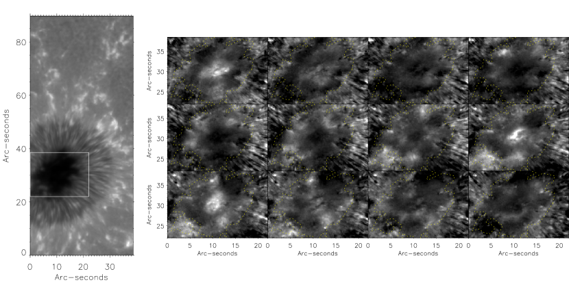
Figure 1: Left: Time average of the intensity in the observed field of view. The area enclosed in the white rectangle is displayed in the right panel. Right: 12 successive snapshots (running from top left to bottom right) of the intensity after subtracting a 20-frame running mean and saturating the scale to show the umbral emission. The yellow dotted lines show the umbra-penumbra boundary as a reference.

2 Observations and data reduction

The observations were taken on 2008 March 29^th at 11:53 UT using the broadband filter of the Solar Optical Telescope onboard the Hinode spacecraft. For details on the instrumentation see Tsuneta et al. (2008). We observed time series of the sunspot in active region number NOAA 10988, located at coordinates (-501”,-104”) from disk center. The time cadence was 20 s. The SOT broadband filter for the Ca II H line has a pass-band of 0.3 nm. Standard reduction procedures, including flatfield and dark current correction, were applied. The time span of our dataset is of approximately 1 hour and 4 minutes. The original series contains some bad frames (i.e., frames with no data in all or part of the field of view) which we avoid by using only a smaller subset of 40 minutes. In this manner we work with a continuous good data set of homogeneous quality and regular sampling. The diffraction limit of the telescope at this wavelength is approximately 0.2”, which is only slightly under-sampled by the pixel size (after binning) of 0.11”. Therefore, our spatial resolution is 0.22” and this figure is of course constant through the entire series.

3 Results

The field of view of our observation can be seen in Figure 1 (left panel). It encompasses most of the sunspot and some of the surrounding moat. In this paper we shall focus on the umbra, in particular the sub-field indicated by the white rectangle in the figure. The right panel of the figure shows a sequence of successive snapshots to give the reader an idea of the complex and intricate patterns found, as well as their very vigorous dynamics. In order to enhance the contrast and present the oscillatory behavior clearly in this and the following figures, we have subtracted a running mean from each snapshot. The mean that we subtract is composed of 20 frames (spanning 400 seconds) around the snapshot under consideration. This procedure is very similar to the one used by Rouppe van der Voort et al. (2003). The umbra-penumbra boundary is overlaid in yellow (dotted line) for reference. The series presented in the figure shows 12 successive snapshots, from top left to bottom right, covering 4 minutes of real time. The dominant oscillation period in the umbra is approximately 3 minutes (see below).

The figure shows some hints of the complex behavior of the umbral dynamics which are more clearly appreciated by viewing the data as a movie. We have included it as an mpeg file with the electronic version of this paper. Umbral flashes are visible occasionally at different locations, some times near the center of the umbra and others near the umbra-penumbra boundary. A more diffuse (but still structured) bright component can be seen moving very rapidly. These motions are unlikely to be actual plasma motions because they would be unrealistically fast ($\sim$100 km s^-1) and the associated Doppler shifts would have been observed already in observations away from the disk center. Most likely the apparent motion is simply caused by the wavefront reaching the line formation height at different times in different locations.

The changes in the diffuse bright component are so fast that they are under-sampled by our 20 s cadence. It is then impossible to track a feature as it moves around because the whole structure has changed from one snapshot to the next. When one watches the movies, the eye tends to interpret the motion as a wave moving around and bouncing off of the umbra-penumbra boundary or the relatively bright structures that protrude into the umbra. However, given that the presumed propagation is under-sampled in time, this might just be an illusion. This component is probably the same that Rouppe van der Voort et al. (2003) describe as arches emanating radially from the flashes. However, we do not see that morphology or behavior in our data. Perhaps the differences in spatial resolution (better in our case) or the time sampling (better in their case) are responsible for the discrepancy. In any case, one should be careful not to over-interpret the sequence of images.

The visual appearance of the movie is very chaotic in the umbra whereas the penumbra exhibits a much smoother behavior. Very fine penumbral filaments are clearly visible in the data, swaying with a slow and smooth oscillation pattern (probably running penumbral waves, described by Nye & Thomas 1974). When umbral flashes occur, they exhibit fine structure. They are actually made of a mixture of bright and dark dots.

Sometimes, however, the bright emission of a flash exhibits filamentary structure. An example is given in Fig 2 (right), where one such structure (marked with arrow “B”) appears in the second frame (top right), remains in the third (bottom left) although the brightening has moved towards the bottom of the figure, and finally has already disappeared by the fourth frame (bottom right). Actually, this figure shows two distinct filament systems. One, around coordinates (8”,25”), marked with arrow “A” in the figure, is nearly oriented along the $y$-axis and is extremely thin. In fact, it is barely resolved in our data and is likely to have even finer structure. The other one, mentioned above, is around coordinates (9”,26”) and marked with arrow “B” in the figure. This second system is more prominent and shows four thick filaments that are still visible in the third frame (identified by the numbers next to them). Figure 3 shows a cross plot with the intensity fluctuation along a line perpendicular to the filaments. We can see that the contrast is not very high, except for filament number 3, which makes it rather hard to discern the structure in the grayscale panels.

We computed the horizontal speed of the brightenings in the four thick filaments as they moved from the second to the third frame of Figure 2, obtaining (from 1 to 4) the following values in km s^-1: 23$\pm$4, 20$\pm$2, 33$\pm$1 and 27$\pm$3. The uncertainty is estimated as the difference in speeds obtained for different points along the same filament. Some of the speeds obtained differ in a statistically significant manner, which may be an indication of differences in field geometry and, possibly, in the wave propagation paths. The speeds are much larger than the vertical Doppler velocities observed in umbral flashes (Beckers & Tallant 1969; Socas-Navarro et al. 2001) so it is unlikely that we are seeing an actual motion of plasma along the field lines.

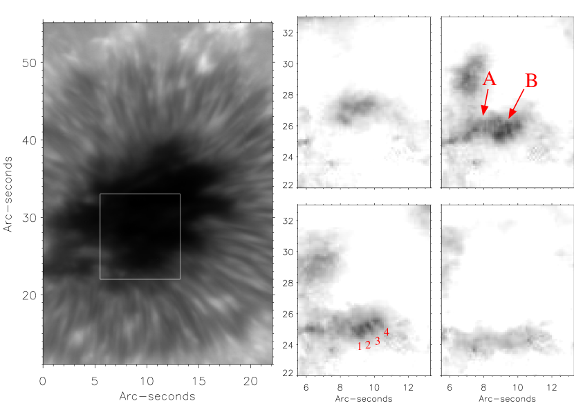
Figure 2: Left: Field of view analyzed in the right panel. Right: 4 successive snapshots showing the propagation of a wavefront inside a filamentary structure. A 20-frame running median has been subtracted from the data. The grey scale has been inverted to show a negative for better viewing. Dark structures in the figure are actually bright and the white background is actually dark.

Figure 3: Cut perpendicular to the direction defined by the filaments marked with arrow “B” in Figure 2. The curve shows the intensity after subracting a 20-frame median in units of the quiet Sun average continuum. The positions of the four filaments labeled with numbers in Figure 2 are shown with vertical dotted lines.

The presence of filaments whose geometry has a significant horizontal component inside the umbra is certainly puzzling. The filament system seen in Fig 2 has a horizontal extension of about 2,000 km. Even taking a conservatively large range for the formation height of the Ca H line core of 1,000 km (the response functions of Carlsson et al. 2007 in the Fontenla et al. 1990 C model would indicate more like $\sim$500 km), the filament orientation must be nearly horizontal. Spanning 2,000 km in the horizontal direction and less than 1,000 km in the vertical, they would deviate less than 25^o from the horizontal. However, we do not make a strong claim in this sense because one has to be careful with such estimates as the formation height is only a meaningful concept in a plane-parallel 1D atmospheric model.

This filamentary system is seen persistently at other times, whenever a strong brightening occurs at this location (for instance, see frames number 32, 49, 56 or 156 in the movie). It is almost as if the umbral flashes acted as a spotlight that moves around the dark umbra and allows us to see things as it illuminates here and there. Figure 4 shows a different filamentary system. The top right figure has been saturated to show in detail the structure of the umbral flash and the filaments that emanate almost radially from the top (pointed by arrow “C”). The bottom right figure has been enhanced to show the filaments emanating from the weaker brightening to the left of the main one (pointed by arrow “D”). These weaker filaments appear to be oriented radially from a common center at coordinates (8”, 32”) approximately.

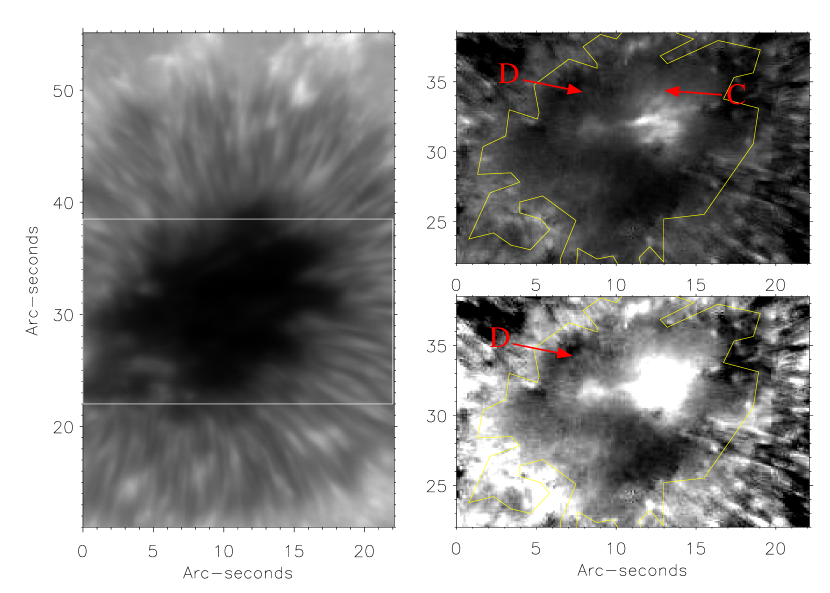
Figure 4: Left: Field of view analyzed in the right panel. Right: Snapshot showing filamentary structure around an umbral flash. A 20-frame running median has been subtracted from the data. The top and bottom images are the same but with different levels of saturation of the grey scale to show different details.

There was one instance where we detected a bright flash that started as a compact emission and then propagated outwards forming a ring (see Fig 5). This flash appears to be near the center of one of the umbral cores and perhaps what we see here is the propagation along field lines fanning out. The propagation speed in this case is 33.5$\pm$3.5 km s^-1, very close to what we had before for the propagation along the filaments in Fig 2. The difference with the Doppler velocity measured in flashes suggests again that this is not an actual motion of material.

Figure 5: Left: Field of view analyzed in the right panel. Right: Two successive snapshots showing the propagation of an umbral flash forming a ring-like structure around the origin.

A Fourier analysis of the intensity oscillation shows that the umbra does not oscillate as a whole (see Figure 6). Instead, it is divided into smaller regions (resembling the umbral cores) inside which the oscillation has a similar dominant frequency. This property, however, can vary abruptly from one region to another. Such subdivision of the umbra into smaller oscillating elements had already been observed before (Lites 1986; Aballe Villero et al. 1993). Part of the variation in the dominant frequency is likely a reflection of the gradient in field inclination across the umbra (McIntosh & Jefferies 2006).

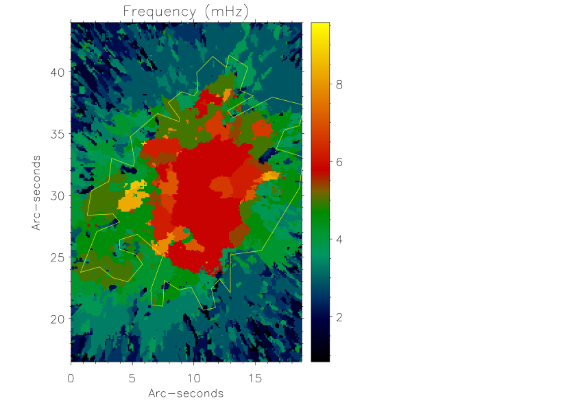
Figure 6: Spatial distribution of the dominant oscillation frequency.

4 Conclusions

We have presented new observations of the umbral chromosphere that finally prove the existence of very fine structure in umbral flashes, as had been anticipated by Socas-Navarro et al. (2000b) and Centeno et al. (2005) based on indirect spectroscopic evidence. Using Hinode’s unique capabilities of very high spatial resolution and time stability, it is now possible to actually see such structure directly. Whether the dark component seen here can be identified with the cool component at rest described in those papers still remains to be confirmed.

To our surprise, we have found evidence for filamentary structure inside the umbra with an important horizontal component (if not nearly horizontal), which is difficult to understand in terms of the simple cartoon picture of a theoretician’s spot. Once more, while simple idealized models are an excellent tool to understand global properties, reality is also rich in intricate details that need to be studied carefully as well.

Clearly, the nature and properties of the filaments deserve further study. Ideally one would like to have Stokes spectroscopy in order to infer the actual orientation of the magnetic field. Unfortunately, no instrument exists today that can do spectro-polarimetry of a Ca II line with the necessary spatial resolution ($\sim$0.2”). Hopefully, 2D imaging filter-polarimeters such as IBIS (Cauzzi et al. 2006) or CRISP (Scharmer et al. 2008) may be able to accomplish this in the near future (but observing the infrared triplet, not the H line).

Perhaps even more mysterious is the existence of fine structure in the chromospheric oscillation. One would think that it must be the reflection of fine structure in the lower layers (possibly below the photosphere) where the waves are excited. Numerical simulations indicate that, in an umbra, waves must propagate upwards in the vertical direction and are channeled by the field lines (Bogdan et al. 2003). The photospheric magnetic field appears even at very high resolution to be very homogeneous and vertically oriented. Therefore, the field cannot be responsible for the inhomogeneities in the oscillation and the source must be in the excitation mechanism itself.

References

- Aballe Villero et al. (1993) Aballe Villero, M. A., Marco, E., Vazquez, M., & Garcia de La Rosa, J. I. 1993, A&A, 267, 275
- Beckers & Tallant (1969) Beckers, J. M., & Tallant, P. E. 1969, Solar Phys., 7, 351
- Bellot Rubio (2007) Bellot Rubio, L. R. 2007, in Highlights of Spanish Astrophysics IV, ed. F. Figueras, J. M. Girart, M. Hernanz, & C. Jordi, 271–+
- Bogdan et al. (2003) Bogdan, T. J., Carlsson, M., Hansteen, V. H., McMurry, A., Rosenthal, C. S., Johnson, M., Petty-Powell, S., Zita, E. J., Stein, R. F., McIntosh, S. W., & Nordlund, Å. 2003, ApJ, 599, 626
- Carlsson et al. (2007) Carlsson, M., Hansteen, V. H., de Pontieu, B., McIntosh, S., Tarbell, T. D., Shine, D., Tsuneta, S., Katsukawa, Y., Ichimoto, K., Suematsu, Y., Shimizu, T., & Nagata, S. 2007, Pub. Astron. Soc. Japan, 59, 663
- Cauzzi et al. (2006) Cauzzi, G., Cavallini, F., Reardon, K., Berrilli, F., Rimmele, T., & IBIS Team. 2006, in Bulletin of the American Astronomical Society, Vol. 38, Bulletin of the American Astronomical Society, 226–+
- Centeno et al. (2005) Centeno, R., Socas-Navarro, H., Collados, M., & Trujillo Bueno, J. 2005, ApJ, 635, 670
- Fontenla et al. (1990) Fontenla, J. M., Avrett, E. H., & Loeser, R. 1990, ApJ, 355, 700
- Kneer et al. (1981) Kneer, F., Mattig, W., & v. Uexkuell, M. 1981, A&A, 102, 147
- Kosugi et al. (2007) Kosugi, T., Matsuzaki, K., Sakao, T., Shimizu, T., Sone, Y., Tachikawa, S., Hashimoto, T., Minesugi, K., Ohnishi, A., Yamada, T., Tsuneta, S., Hara, H., Ichimoto, K., Suematsu, Y., Shimojo, M., Watanabe, T., Shimada, S., Davis, J. M., Hill, L. D., Owens, J. K., Title, A. M., Culhane, J. L., Harra, L. K., Doschek, G. A., & Golub, L. 2007, Solar Phys., 243, 3
- Lites (1986) Lites, B. W. 1986, ApJ, 301, 992
- López Ariste et al. (2001) López Ariste, A., Socas-Navarro, H., & Molodij, G. 2001, ApJ, 552, 871
- McIntosh & Jefferies (2006) McIntosh, S. W., & Jefferies, S. M. 2006, ApJ, 647, L77
- Nagashima et al. (2007) Nagashima, K., Sekii, T., Kosovichev, A. G., Shibahashi, H., Tsuneta, S., Ichimoto, K., Katsukawa, Y., Lites, B., Nagata, S., Shimizu, T., Shine, R. A., Suematsu, Y., Tarbell, T. D., & Title, A. M. 2007, Pub. Astron. Soc. Japan, 59, 631
- Nye & Thomas (1974) Nye, A. H., & Thomas, J. H. 1974, Solar Phys., 38, 399
- Rouppe van der Voort et al. (2003) Rouppe van der Voort, L. H. M., Rutten, R. J., Sütterlin, P., Sloover, P. J., & Krijger, J. M. 2003, A&A, 403, 277
- Scharmer et al. (2007) Scharmer, G. B., Langhans, K., Kiselman, D., & Löfdahl, M. G. 2007, in Astronomical Society of the Pacific Conference Series, Vol. 369, New Solar Physics with Solar-B Mission, ed. K. Shibata, S. Nagata, & T. Sakurai, 71–+
- Scharmer et al. (2008) Scharmer, G. B., Narayan, G., Hillberg, T., de la Cruz Rodriguez, J., Lofdahl, M. G., Kiselman, D., Sutterlin, P., van Noort, M., & Lagg, A. 2008, ArXiv e-prints
- Schüssler & Vögler (2006) Schüssler, M., & Vögler, A. 2006, ApJ, 641, L73
- Shimizu et al. (2008) Shimizu, T., Nagata, S., Tsuneta, S., Tarbell, T., Edwards, C., Shine, R., Hoffmann, C., Thomas, E., Sour, S., Rehse, R., Ito, O., Kashiwagi, Y., Tabata, M., Kodeki, K., Nagase, M., Matsuzaki, K., Kobayashi, K., Ichimoto, K., & Suematsu, Y. 2008, Solar Phys., 249, 221
- Socas-Navarro et al. (2000a) Socas-Navarro, H., Trujillo Bueno, J., & Ruiz Cobo, B. 2000a, ApJ, 544, 1141
- Socas-Navarro et al. (2000b) —. 2000b, Science, 288, 1396
- Socas-Navarro et al. (2001) —. 2001, ApJ, 550, 1102
- Tsuneta et al. (2008) Tsuneta, S., Ichimoto, K., Katsukawa, Y., Nagata, S., Otsubo, M., Shimizu, T., Suematsu, Y., Nakagiri, M., Noguchi, M., Tarbell, T., Title, A., Shine, R., Rosenberg, W., Hoffmann, C., Jurcevich, B., Kushner, G., Levay, M., Lites, B., Elmore, D., Matsushita, T., Kawaguchi, N., Saito, H., Mikami, I., Hill, L. D., & Owens, J. K. 2008, Solar Phys., 249, 167
- Turova et al. (1983) Turova, I. P., Teplitskaia, R. B., & Kuklin, G. V. 1983, Solar Phys., 87, 7
- Tziotziou et al. (2007) Tziotziou, K., Tsiropoula, G., Mein, N., & Mein, P. 2007, A&A, 463, 1153
- Tziotziou et al. (2002) Tziotziou, K., Tsiropoula, G., & Mein, P. 2002, A&A, 381, 279
- Wittmann (1969) Wittmann, A. 1969, Solar Phys., 7, 366