Stochastic excitation of nonradial modes
II. Are solar asymptotic gravity modes detectable?

Abstract

Context. Detection of solar gravity modes remains a major challenge to our understanding of the inner parts of the Sun. Their frequencies would enable the derivation of constraints on the core physical properties, while their amplitudes can put severe constraints on the properties of the inner convective region.

Aims. Our purpose is to determine accurate theoretical amplitudes of solar g modes and estimate the SOHO observation duration for an unambiguous detection of individual modes. We also explain differences in theoretical amplitudes derived from previous works.

Methods. We investigate the stochastic excitation of modes by turbulent convection, as well as their damping. Input from a 3D global simulation of the solar convective zone is used for the kinetic turbulent energy spectrum. Damping is computed using a parametric description of the nonlocal, time-dependent, convection-pulsation interaction. We then provide a theoretical estimation of the intrinsic, as well as apparent, surface velocity.

Results. Asymptotic g-mode velocity amplitudes are found to be orders of magnitude higher than previous works. Using a 3D numerical simulation from the ASH code, we attribute this to the temporal-correlation between the modes and the turbulent eddies, which is found to follow a Lorentzian law rather than a Gaussian one, as previously used. We also find that damping rates of asymptotic gravity modes are dominated by radiative losses, with a typical life time of $3\times 10^{5}$ years for the $\ell=1$ mode at $\nu=60\,\mu$Hz. The maximum velocity in the considered frequency range (10-100 $\mu$Hz) is obtained for the $\ell=1$ mode at $\nu=60\,\mu$Hz and for the $\ell=2$ at $\nu=100\,\mu$Hz. Due to uncertainties in the modeling, amplitudes at maximum i.e. for $\ell=1$ at 60 $\mu$Hz can range from 3 to 6 mm s^-1. The upper limit is too high, as g modes would have been easily detected with SOHO, the GOLF instrument, and this sets an upper constraint mainly on the convective velocity in the Sun.

1 Introduction

The pioneer works of Ulrich (1970) and Leibacher & Stein (1971) led to the identification of the solar five-minutes oscillations as global acoustic standing waves ($p$ modes). Since then, successful works have determined the Sun internal structure from the knowledge of its oscillation frequencies (e.g., Christensen-Dalsgaard 2004). However, $p$ modes are not well-suited to probing the deepest inner part of the Sun. On the other hand, $g$ modes are mainly trapped in the radiative region and are thus able to provide information on the properties of the central part of the Sun ($r<0.3\,R_{\odot}$) (e.g., Turck-Chièze et al. 2001; Christensen-Dalsgaard 2006). As $g$ modes are evanescent in the convective region, their amplitudes are expected to be very low at the photosphere and above, where observations are made, making their detection is thus quite a challenge for more than $30$ years.

The first claims of detection of solar gravity modes began with the work of Severnyi et al. (1976) and Brookes et al. (1976). Even after more than ten years of observations from SOHO, there is still no consensus about detection of solar $g$ modes. Most of the observational efforts have been focused on low-order $g$ modes motivated by a low the granulation noise (Appourchaux et al. 2006; Elsworth et al. 2006) and by previous theoretical estimates of $g$-mode amplitudes (e.g., Turck-Chièze et al. 2004; Kumar et al. 1996). Recently, García et al. (2007) have investigated the low-frequency domain, with the hope of detecting high radial-order $g$ modes. The method looked for regularities in the power spectrum, and the authors claim to detect a periodicity in accordance with what is expected from simulated power spectra. The work of García et al. (2007) present the advantage of exploring a different frequency domain ($\nu\in[25;140]\mu$Hz) more favorable to a reliable theoretical estimation of the $g$-mode amplitudes, as we will explain later on.

Amplitudes of $g$ modes, as $p$ modes, are believed to result from a balance between driving and damping processes in the solar convection zone. Two major processes have been identified as stochastically driving the resonant modes in the stellar cavity. The first is related to the Reynolds stress tensor, the second is caused by the advection of turbulent fluctuations of entropy by turbulent motions. Theoretical estimations based on stochastic excitation have been previously obtained by Gough (1985) and Kumar et al. (1996). Gough (1985) made an order of magnitude estimate based on an assumption of equipartition of energy as proposed by Goldreich & Keeley (1977b). He found a maximum velocity around $0.5\,\textrm{mm\,s}^{-1}$ for an $\ell=1$ mode at $\nu\approx 100\,\mu$Hz. Kumar et al. (1996) used a different approach based on the Goldreich et al. (1994) modeling of stochastic excitation by turbulent convection, as well as an estimating of the damping rates (Goldreich & Kumar 1991) that led to a surface velocity near $0.01\,\textrm{mm\,s}^{-1}$ for the $\ell=1$ mode at $\nu\approx 100\,\mu$Hz. The results differ from each other by orders of magnitude, as pointed out by Christensen-Dalsgaard (2002b). Such differences remain to be understood. One purpose of the present work is to carry out a comprehensive study of both the excitation and damping rates of asymptotic $g$ modes. Our second goal is to provide theoretical oscillation mode velocities, , as reliably as possible. Note, however, that penetrative convection is another possible excitation mechanism (Andersen 1996; Dintrans et al. 2005), but it is beyond the scope of this paper.

Damping rates are computed using the Grigahcène et al. (2005) formalism that is based on a non-local time-dependent treatment of convection. We will show that, contrary to $p$ modes and high frequency $g$ modes, asymptotic $g$-mode (i.e low frequency) damping rates are insensitive to the treatment of convection. This then removes most of the uncertainties in the estimated theoretical oscillation mode velocities. Consequently, we restrict our investigation to low-frequency gravity modes. Stochastic excitation is modeled in the same way as in Belkacem et al. (2008), which is a generalization to non-radial modes of the formalism developed by Samadi & Goupil (2001) and Samadi et al. (2003b, a), for radial modes. As in the case of $p$-modes, the excitation formalism requires knowing the turbulent properties of the convection zone, but unlike $p$ modes, the excitation of gravity modes is not concentrated towards the uppermost surface layers. One must then have some notion about the turbulent properties across the whole convection zone. Those properties will be inferred from a 3-D numerical simulation provided by the ASH code (Miesch et al. 2008).

The paper is organized as follows. Section 2 briefly recalls our model for the excitation by turbulent convection and describes the input from a 3D numerical simulation. Section 3 explains how the damping rates are computed. Section 4 gives our theoretical results on the surface velocities of asymptotic $g$ modes and compares them with those from previous works. Section 5 provides the apparent surface velocities, which take disk integrated effects and line formation height into account. These quantities can be directly compared with observations. We then discuss our ability to detect these modes using data from the GOLF instrument onboard SOHO as a function of the observing duration. The discussion is based on estimations of detection threshold and numerical simulations of power spectra. In Sect. 6., uncertainties on the estimated theoretical and apparent velocities, due to the main uncertainties in our modeling, are discussed. Finally, conclusions are provided in Sect. 7.

2 Excitation by turbulent convection

The formalism we used to compute excitation rates of non-radial modes was developed by Belkacem et al. (2008) who extended the work of Samadi & Goupil (2001) developed for radial modes to non-radial modes. It takes the two sources into account that drive the resonant modes of the stellar cavity. The first is related to the Reynolds stress tensor and the second one is caused by the advection of the turbulent fluctuations of entropy by the turbulent motions (the ”entropy source term”). Unlike for $p$ modes, the entropy source term is negligible for $g$ modes. We numerically verified that it is two to four orders of magnitude lower than the Reynolds stress contribution depending on frequency. This is explained by the entropy contribution being sensitive to second-order derivatives of the displacement eigenfunctions in the superadiabatic region where entropy fluctuations are localized. As the gravity modes are evanescent in the convection zone, the second derivatives of displacement eigenfunctions are negligible and so is the entropy contribution.

The excitation rate, $P$, then arises from the Reynolds stresses and can be written as (see Eq. (21) of Belkacem et al. 2008)

$$P =\frac{\pi^{3}}{2I}\int_{0}^{M}\textrm{d}m\,\rho_{0}\,R(r)\int_{0}^{+\infty}\textrm{d}k\;\mathcal{S}_{k}$$ (1)

$$\mathcal{S}_{k} =\frac{1}{k^{2}}\int_{-\infty}^{+\infty}\textrm{d}\omega\leavevmode\nobreak\ E^{2}(k)\leavevmode\nobreak\ \chi_{k}(\omega+\omega_{0})\leavevmode\nobreak\ \chi_{k}(\omega)$$ (2)

where $m$ is the local mass, $\rho_{0}$ the mean density, $\omega_{0}$ the mode angular frequency, $I$ the mode inertia, $\mathcal{S}_{k}$ the source function, $E(k)$ the spatial kinetic energy spectrum, $\chi_{k}$ the eddy-time correlation function, and $k$ the wavenumber. The term $R(r)$ depends on the eigenfunction, its expression is given in Eq. (23) of Belkacem et al. (2008), i.e

$$R(r) = {16\over 15}\leavevmode\nobreak\ \left|\frac{\textrm{d}\xi_{r}}{\textrm{d}r}\right|^{2}+{44\over 15}\leavevmode\nobreak\ \left|\frac{\xi_{r}}{r}\right|^{2}+\frac{4}{5}\left(\frac{\xi^{*}_{r}}{r}\frac{\textrm{d}\xi_{r}}{\textrm{d}r}+c.c\right)$$ (3)

$$+ \leavevmode\nobreak\ L^{2}\left({11\over 15}\leavevmode\nobreak\ \left|\zeta_{r}\right|^{2}-{22\over 15}(\frac{\xi_{r}^{*}\xi_{h}}{r^{2}}+c.c)\right)$$

$$- {2\over 5}L^{2}\left(\frac{\textrm{d}\xi^{*}_{r}}{\textrm{d}r}{\xi_{h}\over r}+c.c\right)$$

$$+ \left|\frac{\xi_{h}}{r}\right|^{2}\left(\frac{16}{15}L^{4}+\frac{8}{5}{\cal F}_{\ell,|m|}-\frac{2}{3}L^{2}\right)\,,$$

where we have defined

$$L^{2} = \ell(\ell+1)$$ (4)

$$\zeta_{r} \equiv \frac{\textrm{d}\xi_{h}}{\textrm{d}r}+\frac{1}{r}(\xi_{r}-\xi_{h})$$ (5)

$${\cal F}_{\ell,|m|} = \frac{|m|(2\ell+1)}{2}\left(L^{2}-(m^{2}+1)\right)\,,$$ (6)

and $\xi_{r},\xi_{h}$ are the radial and horizontal components of the fluid displacement eigenfunction ($\@vec{\xi}$), and $\ell,m$ represent the degree and azimuthal number of the associated spherical harmonics.

2.1 Numerical computation of theoretical excitation rates

In the following, we compute the excitation rates of $g$ modes for a solar model. The rate ($P$) at which energy is injected into a mode per unit time is calculated according to Eq. (1). Eigenfrequencies and eigenfunctions are computed using the adiabatic pulsation code OSC (Boury et al. 1975). The solar structure model used for these computations is obtained with the stellar evolution code CESAM (Morel 1997) for the interior and a Kurucz (1993) model for the atmosphere. The interior-atmosphere matching point is chosen at $\log\tau=0.1$ (above the convective envelope). The pulsation computations use the full model (interior+atmosphere). In the interior model, we used the OPAL opacities (Iglesias & Rogers 1996) extended to low temperatures with the opacities of Alexander & Ferguson (1994) and the CEFF equation of state (Christensen-Dalsgaard & Däppen 1992). Convection is included according to a Böhm-Vitense mixing-length (MLT) formalism (see Samadi et al. 2006, for details), from which the convective velocity is computed. Turbulent pressure is not included (but see discussion in Sect.6).

Apart from the eigenfunctions and the density stratification, Eq. (1) involves both the convective velocity and the turbulent kinetic energy spectrum. To get some insight into the turbulent properties of the inner part of the solar convection zone, we chose to use results from (ASH) 3D numerical simulations. Such a choice was motivated by the uncertainties inherent in the treatment of turbulence by the MLT. The MLT indeed only gives us an estimation of the convective flux but is not able to assess the contributions of all scales involved in turbulent convection. Thus, in the following, the rms convective velocity is taken from the mixing-length theory, while both the spatial and temporal turbulent properties are inferred from the 3D simulation. Then, velocity from the numerical simulation is not used in our calculation. This choice is motivated by the rigid boundary condition at the top of the simulation that results in an unrealistic decrease in the vertical velocity for $r>0.93\,R_{\odot}$.

2.2 The 3D convection simulation

Figure 1: Luminosity flux contributions versus radius, averaged over horizontal surfaces and in time. The solid line corresponds to the enthalpy luminosity ($L_{e}$), the short dashed-line to the radiative luminosity ($L_{r}$), the dotted-dashed line to the kinetic energy luminosity ( $L_{kin}$), the long-dashed line to the total luminosity ($L_{tot}$), and the dot-dashed line correspond to the unresolved eddy luminosity ($L_{ed}$) (Brun et al. 2004). We particularly emphasize the negative kinetic-energy flux that results in a larger convective flux (see text for details).

One way of assessing the dynamical properties of the deep solar turbulent convection zone is to exploit a high resolution numerical simulation such as those performed with the anelastic spherical harmonic (ASH) code (Miesch et al. 2008; Brun et al. 2004). The simulation of global scale turbulent convection used in the present work is discussed in detail in Miesch et al. (2008). The ASH code solves the hydrodynamic anelastic equations within a spherical shell extending from $r=0.71$ up to $r=0.98R_{\odot}$, yielding an overall radial density contrast of 132. Solar values were assumed for the rotation rate and the imposed luminosity. Figure 1 represents the energy flux balance (converted to luminosity and normalized to the solar luminosity) in the simulation. We clearly see how dominant, and overluminous, the convective (enthalpy) flux is in carrying the heat outward. This is mostly due to the strong density contrast and to the corresponding strong asymmetry between up- and downflows yielding a large inward kinetic energy flux (see Miesch et al. 2008 for more details). We have seen above that, in order to compute the excitation rate of the waves, one needs some well-defined physical quantities, such as the kinetic energy spectrum $(E_{k})$ and the eddy time function $({\chi_{k}})$. It is straightforward to deduce these quantities from the 3D simulation as explained in Appendix B. We then directly use $E_{k}$ in Eq. (2) to compute the source function, whereas for $\chi_{k}$ we perform a fit of the 3-D results with a simple analytical expression. In the ASH code, the set of anelastic equations is projected onto spherical harmonics for the horizontal dimensions. This implies that the kinetic energy spectrum is obtained as a function of the spherical degree l . The local wavenumber $k_{h}$ is obtained via the simple expression $k_{h}=\sqrt{{\cal\it l}({\cal\it l}+1)}/r$, with $r$ the shell radius.

2.2.1 Kinetic energy spectrum and time-correlation function

Figure 2: $E(k_{h})$ computed as explained in Appendix. B, for three shell radii that sample the convection zone, as a function of the local horizontal wave number $k_{h}$.

Figure 3: Top: Crosses represent $\chi_{k}(\omega)$ obtained from the 3D simulation at the wave number $k_{0}$ that corresponds to the maximum of $E(k)$, and at the radius $r/R_{\odot}=0.89$. Data are obtained with a time series of duration $\approx 45.83$ days with a sampling time of $4\cdot 10^{4}$ seconds. Analytical functions are normalized so that their integrals are equal to unity. Bottom: The same as the upper panel except that data are obtained with a time series of duration $\sim$ 4.68 days with a sampling time of 800 seconds. The theoretical curves are normalized so that their integrals over frequency equal that of the simulated data.

The kinetic energy spectrum of the total velocity (i.e. the horizontal and vertical components), $E(k_{h})$, is plotted in the top panel of Fig. 2 as a function of the local horizontal wave number $k_{h}$. The rms convective velocity ($u$) increases with $r$, thus explaining that the deeper the layers, the smaller $E(k)$ since $\int\textrm{d}k\,E(k)=1/2\,u^{2}$. In terms of excitation rates, an important issue is the scale at which the spectrum peaks. As pointed out by Miesch et al. (2008), the scale at which the kinetic energy spectrum is maximum is the scale between the downwflows. It is about $58$ Mm at the top of the simulation ($r=0.98\,R_{\odot}$) up to $300$ Mm at the bottom. This is quite different from what is found in the uppermost layers in 3D numerical simulations of the Sun (e.g., Stein & Nordlund 1998), in which the maximum of $E(k)$ is found on a scale around $1$ Mm. Such a difference is explained by the density that strongly decreases in the upper layers.

The time-correlation function ($\chi_{k}$) also plays an important role. Usually, a Gaussian time-correlation function is used (Goldreich et al. 1994; Chaplin et al. 2005). Samadi et al. (2003a) demonstrate that $\chi_{k}$ is reproduced better by a Lorentzian function. They argue that the departure from a Gaussian function can be explained by the presence of plumes in the uppermost part of the convection zone. This result, obtained with 3-D numerical simulations, was then confirmed by confronting solar-$p$ modes excitation rates, computed with Gaussian and Lorentzian functions, with the observational data. It turns out that the Lorentzian function greatly improves the agreement between models and observations. However, the time-correlation function is unknown at deeper layers. The eddy-time correlation function derived from the 3D numerical simulation provided by the ASH code is therefore compared to Gaussian and Lorentzian functions that are respectively defined as

$$\chi_{k}(\omega) =\frac{1}{\omega_{k}\,\sqrt{\pi}}e^{-(\omega/\omega_{k})^{2}}$$ (7)

$$\chi_{k}(\omega) =\frac{1}{\pi\omega_{k}/2}\,\frac{1}{1+\left(2\omega/\omega_{k}\right)^{2}}$$ (8)

with the condition

$$\int_{-\infty}^{+\infty}\chi_{k}(\omega)\textrm{d}\omega=1$$ (9)

where $\omega_{k}$ is its linewidth, defined as

$$\omega_{k}\equiv\,{2\,k\,u_{k}\over\lambda}\;.$$ (10)

where $\lambda$ is a parameter as in Balmforth (1992), the velocity $u_{k}$ of the eddy with wavenumber $k$ is related to the kinetic energy spectrum $E(k_{h})$ by (Stein 1967)

$$u_{k}^{2}=\int_{k}^{2k}dk\,E(k)\;.$$ (11)

Figure 3 presents the comparison between analytical time-correlation functions, computed following the set of Eqs. (7)-(11), and $\chi_{k}$ computed from the 3D numerical simulation. The latter is calculated as described in Appendix. B. The Lorentzian function represents the eddy-time correlation function better than a Gaussian function in the frequency range we are interested in ($\nu\in[20\,\mu\textrm{Hz};110\,\mu\textrm{Hz}]$).

The best fit is found using a sum of a Lorentzian function with $\lambda=3$ and a Gaussian with $\lambda=1/3$ as shown in the top panel of Fig. 3. In the frequency range we are interested in, i.e. at frequencies corresponding to the gravity modes (bottom panel of Fig. 3) the fit reproduces the time-correlation given by the 3-D numerical simulation. We also clearly see that the eddy-time correlation function is very poorly represented by a Gaussian function, which only reproduces very low frequencies that do not significantly contribute to the excitation, then it fails and underestimates $\chi_{k}$ by many order of magnitudes (see Sect. 4.2.2).

The results presented in Fig. 3 are for the depth $r\approx 0.8R_{\odot}$, where excitation is dominant, and for an angular degree corresponding to the maximum of the kinetic energy spectrum ($\ell=40$), whose contribution is dominant in the excitation rates. Those results do not depend on the shell considered but instead on the wavenumber. For very high angular degree ($\ell>300$) we find that $\chi_{k}$ becomes more and more Gaussian. Nevertheless, as shown by Fig. 2, those contributions are negligible compared to large-scale ones.

The value of the parameter $\lambda$ is also of interest. Contrary to the upperlayers where $\lambda=1$ (Samadi et al. 2003b), we find a higher value, $\lambda=3$, that accords with the result of Samadi et al. (2003b) who find that the deeper the layers, the higher this parameter.

2.2.2 The source function

Figure 4 displays the source function ($\mathcal{S}_{k}$, Eq. (1)) as a function of both the angular degree l involved in the summation Eq. (38) and the mode frequency. The function $\mathcal{S}_{k}$ evaluated at two levels, $r=0.95R_{\odot}$ and $r=0.74R_{\odot}$, is shown in order to emphasize the dependence of $\mathcal{S}_{k}$ with the radius. Near the top of the convection zone, $\mathcal{S}_{k}$ is non-negligible at high frequencies ($\nu>50\mu$Hz) and on small scales. From top to bottom, the intensity of the source function decreases such that at the bottom, significant intensities exist only on large scales (small l values) and low frequencies. This behavior corresponds to the evolution of convective elements, i.e turbulent eddies evolve on larger time and spatial scales with depth. Thus, we conclude that high-frequency $g$ modes are mainly excited in the upper layers, whereas low ones are excited deeper; however, the net excitation rate, Eq. (1), is a balance between the eigenfunction shape and the source function.

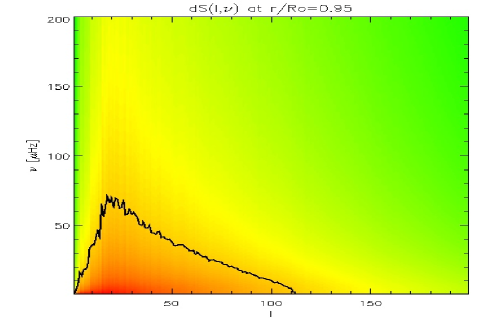
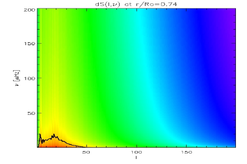
Figure 4: The source function is plotted versus the spherical angular degree (l), and the frequency for two radii: $r=0.95R_{\odot}$ (top panel) and $r=0.74R_{\odot}$ (bottom panel). Bright (red) and dark (blue) tones indicate the high and low intensity of the source function, respectively. The color table is logarithmic. The black line corresponds to an arbitrary contour line that is the same for both panels.

2.3 Excitation rates

Anticipating the following (see Sect. 3), we stress that modes with high angular degree will be highly damped, making their amplitudes very small; hence, we restrict our investigation to low-$\ell$ degrees ($\ell<4$). In Fig 5, we present the excitation rates for low-frequency gravity modes (i.e., $\ell=1,2,3$). By asymptotic modes we denote low-frequency modes ($\nu<100\,\mu$Hz, i.e high-$|n|$ modes) while high frequencies ($\nu>100\,\mu$Hz) correspond to low-$|n|$ modes. At low frequencies ($\nu<100\,\mu$Hz), the excitation rate ($P$) decreases with increasing $\nu$, it reaches a minimum and then at high frequency increases with the frequency. This can be explained by considering the two major contributions to the excitation rate $P$ (Eq. (1) and Eq. (3)) which are the inertia $I$ (in Eq. (1)) and mode compressibility ($\nabla\cdot\xi$, appearing in $R(r)$, Eq. (3)).

Mode inertia decreases with frequency as shown by Fig. 6 since the higher the frequency, the higher up the mode is confined in the upper layers. This then tends to decrease the efficiency of the excitation of low-frequency modes. On the other hand, mode compressibility (Fig. 6) increases with frequency and consequently competes and dominates the effect of mode inertia. Mode compressibility can be estimated as

$$\left|\int_{\Omega}d\Omega\leavevmode\nobreak\ Y_{\ell}^{m}\leavevmode\nobreak\ \@vec{\nabla}\cdot\,\@vec{\xi}\right|\approx\left|\frac{\textrm{d}\xi_{r}}{\textrm{d}r}-\ell(\ell+1)\frac{\xi_{h}}{r}\right|$$ (12)

The mode compressibility is minimum when both terms in Eq. (12) are of the same order. Following Belkacem et al. (2008), one has

$$\left|\frac{\textrm{d}\xi_{r}}{\textrm{d}r}/\frac{\ell(\ell+1)\xi_{h}}{r}\right|\simeq\frac{\sigma^{4}}{\ell(\ell+1)}\quad\textrm{with}\quad\sigma^{2}=\frac{R^{3}}{GM}\omega_{0}^{2}$$ (13)

where $\sigma$ is the dimensionless frequency, $\omega_{0}$ is the angular frequency of the mode, $R$ the Sun radius, and $M$ its mass. According to Eq. (13), mode compressibility is minimum for $\nu\approx 100\,\mu$Hz depending on $\ell$, as shown by Fig. 6. In contrast, in the asymptotic regime ($\nu<100\,\mu$Hz), the modes are compressible and this compressibility increases with decreasing frequency.

It is important to stress that for the asymptotic $g$ modes, in the frequency range $[20;110]\,\mu$Hz, the horizontal contributions in Eq. (3) are dominant. For low-$\ell$ $g$ modes, the dominant contributions come, in Eq. (3), from the component of the mode divergence (see Eq. (12)). Then the ratio of the horizontal to the vertical contributions to Eq. (1) is around a factor five, imposing the use of a non-radial formalism.

Figure 5: Rate ($P$) at which energy is supplied to the modes versus the frequency for modes with angular degree $\ell=1,2$, and $3$. The computation is performed as detailed in Sect. 2.1, using a Lorentzian eddy-time correlation function.

Figure 6: Top: Absolute value of mode compressibility for $\ell=1$ modes versus the frequency, computed for three different layers in the convection zone. Bottom: Mode inertia versus frequency for modes with angular degree $\ell=1,2,3$.

3 Damping rates

To compute theoretical (surface velocities) amplitudes of $g$ modes, knowledge of the damping rates is required.

3.1 Physical input

Damping rates have been computed with the non-adiabatic pulsation code MAD (Dupret 2002). This code includes a time-dependent convection (TDC) treatment described in Grigahcène et al. (2005): it takes into account the role played by the variations of the convective flux, the turbulent pressure, and the dissipation rate of turbulent kinetic energy. This TDC treatment is non-local, with three free parameters $a$, $b$, and $c$ corresponding to the non-locality of the convective flux, the turbulent pressure and the entropy gradient. We take here the values $a=10$, $b=3$, and $c=3.5$ obtained by fitting the convective flux and turbulent pressure of 3D hydrodynamic simulations in the upper overshooting region of the Sun (Dupret et al. 2006c). According to Grigahcène et al. (2005), we introduced a free complex parameter $\beta$ in the perturbation of the energy closure equation. This parameter is introduced to prevent non-physical spatial oscillation of the eigenfunctions. We use here the value $\beta=-0.5i$, which leads to a good agreement between the theoretical and observed damping rates and phase lags in the range of solar pressure modes (Dupret et al. 2006a). The sensitivity of the damping rates to $\beta$ is discussed in Sect. 3.2.1, and we show in next sections that the values of those parameters have no influence on the results since we are interested in low-frequency $g$ modes.

We use the TDC treatment as described in Dupret et al. (2006b), in which the 1D model reproduces exactly the mean convective flux, the turbulent pressure and the mean superadiabatic gradient obtained from a 3D hydrodynamic simulation by Stein & Nordlund (1998), by introducing two fitting parameters, the mixing-length, and a closure parameter (see Dupret et al. 2006b, for details). We also stress that, for low-frequency $g$ modes, particular attention is to be paid to the solution of the energy equation near the center as explained in Appendix A for the $\ell=1$ modes since those dipolar modes present a peculiar behavior near the center that must be properly treated.

3.2 Numerical results for a solar model

3.2.1 Sensibility to the time-dependent treatment of convection

Figure 7: Work integrals for $\ell=1$ and $\ell=2$ modes at $\nu\simeq 60\mu$Hz (top panel) and $\nu\simeq 20\mu$Hz (bottom panel), the surface values give the damping rates $\eta$ in $\mu$Hz.

To understand the contribution of each layer of the Sun in the damping of the $g$ modes, we give the normalized work integral in Fig. 7 in such a way that the surface value is the damping rate $\eta$ (in $\mu$Hz). Results obtained with our TDC treatment (solid lines) and with frozen convection (FC, dashed line) are compared for 4 different modes with $\nu\simeq 60\mu$Hz (top panel) and $\nu\simeq 20\mu$Hz (bottom panel). We see that most of the damping occurs in the inner part of the radiative core. The work integrals obtained with TDC and FC treatments are not very different; hence, the uncertainties inherent in the treatment of the coherent interaction between convection and oscillations do not significantly affect the theoretical damping rates of solar asymptotic $g$ modes. This means that the frozen convection is adapted to low-frequency $g$ modes. This can be explained by paying attention to the ratio $\mathcal{Q}=\omega_{0}/\omega_{c}$, where $\omega_{0}$ is the oscillation frequency and $\omega_{c}$ the convective frequency, defined to be $\omega_{c}=2\pi\Lambda/u_{mlt}$ where $\Lambda$ is the mixing length and $u_{mlt}$ the convective velocity. In the whole solar convective zone $\mathcal{Q}$ is higher than unity except near the surface (the superadiabatic region). However contributions of the surface layer remain small in comparison with the radiative ones for asymptotic $g$ modes (see Fig. 7).

One can thus draw some conclusions

• for high-frequency $g$ modes ($\nu>110\,\mu\textrm{Hz}$), the work integrals and thus the damping rates are sensitive to the parameter $\beta$ that is introduced to model the convection/pulsation interactions because the role of the surface layers in the work integrals becomes important. As a result, the results on the damping rates are questionable for high frequencies since the value of $\beta$ is derived from the observed $p$ modes and that there is no evidence it can be applied safely for $g$ modes.

• in contrast, for low-frequency $g$ modes ($\nu<110\,\mu\textrm{Hz}$), we find that the work integrals and then the damping rates are insensitive to parameter $\beta$. Also, we numerically checked that the damping rates are insensitive to the non-local parameters introduced in Sect. 3.1.

Figure 8: Contributions to the work by the radial radiative flux variation (solid line), the transverse radiative flux variation (dotted line), and the time-dependent convection terms (dashed line), for the mode $\ell=1$, g₁₀ (top panel) and $\ell=1$, g₃₂ (bottom panel). Details are given in the text.

3.2.2 Contributions to the work integral

Figure 8 allows us to investigate the respective roles played by different terms in the damping of the mode. More precisely we consider two modes ($\ell=1$, g₁₀, $\nu\approx 60\,\mu$Hz and $\ell=1$, g₃₂ , $\nu\approx 20\,\mu$Hz) in the frequency interval of interest here and give in Fig. 8 the modulus of:

• the contribution to the work by the radial part of the radiative flux divergence variations (solid line)

  $$dW_{FRr}=\Re\{\left({\delta T\over T}\right)^{*}\,{\partial\delta L_{R}\over\partial x}\}\>{R\over GM^{2}\sigma}\;,$$ (14)

  where $T$ is the temperature, $L_{R}$ the radiative luminosity, $R$ the solar radius, $M$ the solar mass, $x$ the normalized radius, $\sigma$ the real part of the normalized frequency $\sigma=\omega_{0}/(GM/R^{3})^{1/2}$, and $x$ the normalized radius (see Appendix A). Note that $\delta$ denotes the wave Lagrangian perturbations, $\Re$ the real part, and ^∗ the complex conjugate.

• the contribution to the work by the transversal part of the radiative flux divergence variations (dotted line):
  

  $$dW_{FRh}=-\ell(\ell+1)\>\Re\left\{\frac{\delta T^{*}}{T}\left(\frac{\delta T}{xdT/dx}-\frac{\xi_{r}}{r}\right)\right\}\>\frac{RL}{GM^{2}\sigma x}\,;$$ (15)

• the contribution to the work by the time-dependent convection terms (dashed line): $dW_{C}$ (see Sect. 4 of Grigahcène et al. 2005).

Integration of these terms over the normalized radius gives their global contribution to the work performed during one pulsation cycle.

The time-dependent convection terms have a very low weight for both modes in the frequency range $\nu<110\,\mu\textrm{Hz}$. It confirms the conclusion of Sect. 3.2.1 that the damping rates of low-frequency $g$ modes are not dominated by the perturbation of the convective flux,i.e. the interaction convection/oscillation (through the parameter $\beta$). The higher the mode frequency, the higher the integrated convective contribution of the work ($W_{C}$), which becomes dominant for $\nu>110\,\mu\textrm{Hz}$.

While the transverse radiative flux term plays a significant role near the center, the major contribution to the work comes from the radial component of the radiative flux variations. As a result, the radiative damping is the dominant contribution for low-frequency gravity modes.

Figure 9: Theoretical damping rates $\eta$ of g modes of degree $\ell=1,2,3$ as a function of the oscillation frequency in $\mu$Hz.

In Fig. 9, we give the theoretical damping rates $\eta$ of g-modes of degree $\ell=1,2,3$, as a function of the oscillation frequency in $\mu$Hz. We see that for $\nu<110\,\mu$Hz, $\eta$ is a decreasing function of frequency. We find that the frequency dependence is $\eta\propto\omega_{0}^{-3}$. To understand this behavior, we express the integral expression of the damping rate (see Grigahcène et al. 2005, for details) as

$$\eta=\frac{1}{2\,\omega_{0}I}\int_{0}^{M}\mathcal{I}m\left(\frac{\delta\rho}{\rho}^{*}T\delta S\right)\left(\Gamma_{3}-1\right)\textrm{d}m$$ (16)

with

$$I=\int_{0}^{M}\textrm{d}m\;|\@vec{\xi}|^{2}\quad\textrm{and}\quad\left(\Gamma_{3}-1\right)=\left(\frac{\partial lnT}{\partial ln\rho}\right)_{s}$$ (17)

where $\delta\rho,\delta S$ are the perturbations of the density and entropy, respectively, $\rho,T$ are the density and temperature, $\@vec{\xi}$ the eigenfunction, and the star denotes the complex conjugate.

Keeping only the radial contribution of the radiative flux in the energy equation (Eq. (26) ) because it is the dominant contribution, and neglecting the production of nuclear energy ($\epsilon=0$), one gets

$$T\delta S=\frac{i}{\omega_{0}}\frac{\partial\delta L}{\partial m}\,.$$ (18)

This approximation comes from the dominance of the radial contribution of the radiative flux. In addition, in the diffusion approximation

$$\frac{\delta L}{L}=\left(\frac{1}{\left(\textrm{d}T/\textrm{d}r\right)}\frac{\partial\delta T}{\partial r}+2\,\frac{\xi_{r}}{r}+3\,\frac{\delta T}{T}-\frac{\delta\kappa}{\kappa}-\frac{\delta\rho}{\rho}-\frac{\partial\xi_{r}}{\partial r}\right)$$ (19)

Because of the high wavenumber for low-frequency $g$ modes, the term in $\partial\delta T/\partial r$ is very high in Eq. (14), dominates in Eq. (19), and is the main source of damping. This term appears as a second-order derivative in the work integral, and introduces a factor $k_{r}^{2}$ ($k_{r}\approx\sqrt{\ell(\ell+1)}N/(\omega_{0}r)$ is the vertical local wavenumber). Thus, from Eqs. (19), (18), and (16) one obtains $\eta\propto\omega_{0}^{-5}/I$. By using an asymptotic expansion of the eigenfunctions (Christensen-Dalsgaard 2002a), one gets $I\propto\omega_{0}^{-2}$, which permits $\eta\propto\omega_{0}^{-3}$ and explains the behavior of $\eta$ in Fig. 9. The argument is the same for the variation of $\eta$ with the angular degree at fixed frequency becomes it comes from the wave-number dependence $k_{r}^{2}$.

Above  $110\,\mu$Hz, the role of the radiative zone in the mode damping is smaller. There, the damping rates begin to increase with frequency simply because the kinetic energy of the modes decreases faster than the mechanical work.

4 Surface velocities of $g$ modes

4.1 Theoretical (intrinsic) velocities

We compute the mean-squared surface velocity ($v_{s}^{2}$) for each mode as

$$v_{s}^{2}(h) =\left<\int_{\Omega}\Bigl{(}\@vec{v}(\@vec{r},t)\cdot\@vec{v}(\@vec{r},t)\Bigr{)}d\Omega\right>(h)$$ (20)

where $h$ is the height in the stellar atmosphere, $<>$ the time average. Using the expression Eq. (51) in appendix C, one then has

$$v_{s}^{2}(h) =A^{2}\left[v^{2}_{r}(h)+\ell(\ell+1)v^{2}_{h}(h)\right]\,.$$ (21)

The amplitude $A^{2}=(1/2)\left<|a(t)|^{2}\right>$ is given by (Eq. (54)):

$$A^{2}=\frac{P}{2\,\eta\,I\omega_{0}^{2}}$$ (22)

where $<>$ denotes the time average, $I$ the mode inertia, $\eta$ the damping rate, and $v_{r,h}(h)=\omega_{0}\,\xi_{r,h}(h)$ with $\xi_{r}(h)$ and $\xi_{h}(h)$ respectively the radial and horizontal displacement eigenmode components.

In this section, we consider the level of the photosphere $h=R$ with $R$ the radius at the photosphere. Figure 10 presents intrinsic values of the velocities. The behavior of the surface velocities as a function of the angular degree ($\ell$) is mainly due to the damping rates, which rapidly increase with $\ell$; hence, at fixed frequency, the higher the angular degree, the lower the surface velocities. As a consequence, amplitudes are very low for $\ell>3$ . At fixed $\ell$, $v_{s}$ increases with frequency with a slope resulting from a balance between the excitation and damping rates. Nevertheless, modes of angular degree $\ell=1$ exhibit a singular behavior, i.e. a maximum at $\nu\approx 60\,\mu$Hz. This is due to the variation of the slope in the excitation rates (see Fig. 5). In terms of amplitudes, the maximum is found to be $\approx 5\,$mm/s for $\ell=1$ at $\nu\approx 60\,\mu$Hz, which corresponds to the mode with radial order $|n|=10$. It is important to stress that the velocities shown in Fig. 10, are intrinsic values of the modulus that must not be confused with the apparent surface velocities (see Sect. 5), which are the values that can be compared with observed ones.

4.2 Comparison with previous estimations

The theoretical intrinsic velocities obtained in the present work must be compared to previous estimations based on the same assumption that modes are stochastically excited by turbulent convection. All works cited in the next sections deal with intrinsic velocities, i.e. ones not corrected for visibility effects.

4.2.1 Estimation based on the equipartition of energy

The first estimation of $g$-mode amplitudes was performed by Gough (1985), who found a maximum of velocity of about $0.5\,\textrm{mm\,s}^{-1}$ for the $\ell=1$ mode at $\nu\approx 100\,\mu$Hz. Gough (1985) used the principle of equipartition of energy, which consists in equating the mode energy (${\cal E}$) with the kinetic energy of resonant eddies whose lifetimes are close to the modal period. This ”principle” has been theoretically justified for $p$ modes, by Goldreich & Keeley (1977b) assuming that the modes are damped by eddy viscosity. They found that the modal energy to be inversely proportional to the damping rate, $\eta$, and proportional to an integral involving the term $E_{\lambda}\,v_{\lambda}\,\lambda$ where $E_{\lambda}\equiv(1/2)\,m_{\lambda}\,v_{\lambda}^{2}$ is the kinetic energy of an eddy with size $\lambda$, velocity $v_{\lambda}$, and mass $m_{\lambda}=\rho\,\lambda^{3}$ (see Eq. (46) of Goldreich & Keeley 1977b). Using a solar model, they show that the damping rates of solar $p$ modes are dominated by turbulent viscosity and that the damping rates are accordingly proportional to the eddy-viscosity, that is, $\eta\propto v_{\lambda}\,\lambda$ (see Eq. (6) of Goldreich & Keeley 1977a). Hence, after some simplifying manipulations, Goldreich & Keeley (1977b) found the modal energy to be (see their Eq. (52))

$$\mathcal{E}\approx 0.26\,E_{\lambda}=0.13\,m_{\lambda}\,v_{\lambda}^{2}\;.$$ (23)

This principle then was used by Christensen-Dalsgaard & Frandsen (1983) for $p$ modes and Gough (1985) for solar $g$ modes. However, as mentioned above, the result strongly depends on the way the modes are damped, and for asymptotic $g$ modes there is no evidence that this approach can be used and in particular, as shown in this work, if the damping is dominated by radiative losses.

4.2.2 Kumar et al. (1996)’s formalism

Another study was performed by Kumar et al. (1996), which was motivated by a claim of $g$-mode detection in the solar wind (Thomson et al. 1995). Computations were performed using the Goldreich et al. (1994) formalism; both turbulent and radiative contributions to the damping rates were included as derived by (Goldreich & Kumar 1991) who obtained mode lifetimes around $10^{6}\,\textrm{yrs}$. This is not so far from our results (see Fig 9). Kumar et al. (1996) found that the theoretical (i.e. not corrected for visibility factors) surface velocity is around $10^{-2}\,\textrm{cm}\,\textrm{s}^{-1}$ near $\nu=200\,\mu\textrm{Hz}$ for $\ell=1$ modes. However, as shown in Sect. 3, the results for this frequency range are very sensitive to the convective flux perturbation in the damping rate calculations. Thus, we do not discuss the result obtained for those frequencies.

More interesting for our study, Kumar et al. (1996) also found very low velocities ($10^{-2}\,\textrm{mm}\,\textrm{s}^{-1}$) for $\nu<100\,\mu\textrm{Hz}$. This is significantly lower than what we find. However, the efficiency of the excitation strongly depends on how the eddies and the waves are temporally-correlated. As already explained in Sect.2.1, the way the eddy-time correlation function is modeled is crucial since it leads to major differences between, for instance, a Gaussian and a Lorentzian modeling. The Goldreich & Keeley (1977b) approach, from which Kumar et al. (1996)’s formulation is derived, implicitly assumes that the time-correlation between the eddies is Gaussian. The present work (as explained in Sect. 2.1) assumes a Lorentzian for the time correlation function $\chi_{k}$, which results in $v=3$ mm/s in amplitude for $\ell=1$ mode at $\nu\approx 60\,\mu$Hz (Sect. 4.1).

We performed the same computation but now assuming $\chi_{k}$ to be Gaussian (Eq. (7)) and using a Kolmogorov spectrum as in Kumar et al. (1996). In that case (see Fig. 10), we find velocities of the order of $10^{-2}\,mm\,s^{-1}$ for $\ell=1$ which agree with the result of Kumar et al. (1996), which is significantly lower than when assuming a Lorentzian.

Figure 10: Top: Theoretical intrinsic surface velocities of g-modes of degree $\ell=1,2,3$ as a function of the oscillation frequency in $\mu$Hz, computed as described in Sect. 4.1 using a Lorentzian $\chi_{k}$. Bottom: Surface velocities of gravity modes of angular degree $\ell=1$ and $\ell=2$ computed using a Gaussian $\chi_{k}$ and a Kolmogorov spectrum to reproduce the results of Kumar et al. (1996).

5 Apparent surface velocities

$m$	0	1	2	3
$\ell$=1	0.117	0.675
$\ell$=2	0.346	0.107	0.437
$\ell$=3	0.06	0.164	0.0552	0.184

Table 1: Values of the visibility coefficient $\alpha_{\ell}^{m}$ of the radial component of the velocity, corresponding to an inclination angle of $\theta_{0}=83^{o}$.

$m$	0	1	2	3
$\ell$=1	0.094	0.540
$\ell$=2	0.833	0.258	1.053
$\ell$=3	0.291	0.649	0.268	0.892

Table 2: Values of the visibility coefficient $\beta_{\ell}^{m}$ of the radial component of the velocity, corresponding to an inclination angle of $\theta_{0}=83^{o}$.

We denote as disk-integrated apparent velocities the values of amplitudes that take both geometrical and limb darkening effects into account. Contrary to solar $p$ modes, one cannot neglect the horizontal component of $\@vec{\xi}$ compared to the vertical one. The observed velocity ($V_{obs}$) is given by the apparent surface velocity $<|V_{app}(r,t)|^{2}>^{1/2}$(see Appendix. C) evaluated at the observed line formation height $h$:

$$V_{obs}=\left({P\over 2\eta I\omega_{0}^{2}}\right)^{1/2}\leavevmode\nobreak\ \left(\alpha_{\ell}^{m}\,v_{r}(h)+\beta_{\ell}^{m}\,v_{h}(h)\right)$$ (24)

where $\alpha_{\ell}^{m}$ and $\beta_{\ell}^{m}$ are the visibility factors defined in Appendix. C.

In Appendix  C we follow the procedure first derived by Dziembowski (1977) and for asymptotic $g$ modes by Berthomieu & Provost (1990). We use a quadratic limb-darkening law following Ulrich et al. (2000) for the Sun with an angle between the rotation axis and the Equator of $83$ degrees. As mentioned above, the apparent velocities are evaluated at the level $h$, i.e. the height above the photosphere where oscillations are measured. Then $h$ is set so as to correspond to the SoHO/GOLF measurements that use the NaD1 and D2 spectral lines, formed at the optical depth $\tau=5.10^{-4}$ (see Bruls & Rutten 1992). The results are presented in Tables 1 and 2 for angular degrees $\ell=1,2,3$.

Figure 11 displays the apparent velocities for modes $\ell=1,2,3$ and $\ell=m$. For a given angular degree, the azimuthal order degree is chosen such that the apparent velocity is maximal. The velocities of the $m=0$ modes are strongly attenuated by the visibility effects, while the $m=\ell$ modes are less sensitive to them. For $\ell=1$ modes, the amplitudes are divided by a factor of two with respect to the intrinsic velocities, while the $\ell=2,3$ mode velocities remain roughly the same. Consequently, our calculations show that both the $\ell=1$ and $\ell=2$ ($m=\ell$) are the most probable candidates for detection with amplitudes $\approx 3$ mm s^-1.

Figure 11: Apparent surface velocities for $g$ modes of degree $\ell=1,2,3$ as a function of the oscillation frequency in $\mu$Hz (visibility factors are taken into account).

5.1 Detectability of $g$ modes; only a matter of time

To compare our calculated apparent velocities with observations, we used data from the GOLF spectrometer (Gabriel et al. 2002) onboard the SOHO platform, which performed Doppler-like measurements on the disk-integrated velocity of the Sun, using the Na D lines. We used here a series of 3080 days to estimate the background noise level and compare it to the apparent velocities determined in this work.

A first possible approach is to use some analytical and statistical calculations such as the ones developed by Appourchaux et al. (2000) (Eq. 10). Once a length of observation $T$ (in units of 10⁶s), a frequency range $\Delta\nu$ (in $\mu$Hz), and a level of confidence $p_{det}$ are set, this gives the corresponding signal-to-noise ratio

$$\frac{s_{det}}{<s>}\simeq\ln(T)+\ln(\Delta\nu)-\ln(1-p_{det})\,,$$ (25)

where $s_{det}$ is the power of the signal to be detected, and $<s>$ the local power of the noise. This means that any peak in the frequency range $\Delta\nu$ above this ratio has a probability $p_{det}$ of not being due to noise. Choosing a frequency range of $\Delta\nu=10\mu$Hz centered on the frequency of the highest expected velocities (60$\mu$Hz) sets the background level at $\approx$ 500 (m s${}^{-1})^{2}/$Hz. Equation (25) gives an amplitude of $5.2\leavevmode\nobreak\ mm\,s^{-1}$ for a detection with a confidence level $p_{det}$ of 90% for 15 years of observation, $4.6\leavevmode\nobreak\ mm\,s^{-1}$ for 20 years, and $3.8\leavevmode\nobreak\ mm\,s^{-1}$ for 30 years.

Figure 12: Simulated spectrum for an observation length of 30 years, in Case 1. The dashed line indicates the level of detection (see text and Eq. 25). The vertical lines indicate the frequencies of the simulated modes. Here, only one mode is above the detection level. Bottom: Average number and standard deviation (from the 100 realizations) of modes detected in simulations versus the length of observation for the three cases (see text). Above the hashed region (less than four peaks detected), one can consider the detection to be unambiguous. The upper curve corresponds to the case 3 ($A_{\rm max}=2A$), the middle one to case 2 ($A_{\rm max}=1.5A$), and the lower one to case 1 ($A_{\rm max}=A$).

However, this approach has to be repeated for each mode (with its own proper noise level) to have a global view of detection possibilities. To do so, we used simulations. Again relying on the GOLF data to estimate the noise spectrum, we simulated synthetic data including noise and g modes with the apparent velocities as above (and with random phases). Several durations of observation were simulated, from 10 to 30 years. A hundred simulations were performed in each case. The noise level is estimated locally and so is the detection level, following Eq. (25), on the frequency range $[30\,\mu$Hz,$100\,\mu$Hz]. Thus, with a confidence level of 90% and with 7 independent subsets of 10$\mu$Hz, noise is expected to show no peak above the global detection level with a probability of 48%, and to show 1 peak above the global detection level with a probability of 32% (and even 2 peaks in 12% of the realizations). Table 3 lists the average (over 100 simulations) number of peaks detected above the detection level for different observation durations. These simulations were performed using amplitudes $A_{max}$ assuming three different cases:

$\bullet$ Case 1: we assumed for $A_{max}$ the apparent surface velocity amplitudes calculated above, $A$.

Due to uncertainties in the theoretical modeling (as discussed in Sect.6), we also assume:

$\bullet$ Case 2: that amplitudes are larger than the amplitudes estimated above by 50% i.e. $A_{max}=1.5\leavevmode\nobreak\ A$

$\bullet$ Case 3: that amplitudes are larger than the amplitudes estimated above by a factor 2 i.e. $A_{max}=2\leavevmode\nobreak\ A$

$A_{max}$	10 years	15 years	20 years	25 years	30 years
$A$	0.8	1.6	0.8	1.4	1.7
$1.5A$	1.4	2.9	4.5	6.5	8.8
$2A$	4.6	8.5	13.4	20.0	21.7

Table 3: Number of peaks above the detection level in the simulated power spectra versus the duration of observation in three cases. In the simulated signal, the modes are given an amplitude $A_{max}$. The 3 cases respectively correspond to $A_{max}$ being the apparent amplitudes $A$ readily stemmed from our calculation, $A_{max}=1.5A$ and $A_{max}=2A$. The last two cases take into account that uncertainties in the modeling globally tend to underestimate the amplitudes as discussed in Sect.6.

Cases 1 and 3 are the two limits of this exercise. The number of detected peaks in Case 3 shows that the predicted amplitudes cannot be overestimated by a factor of two, because in this case, the solar g modes would have already been detected without doubt. Case 1 sets a lower limit, because in this case, even with longer (30 years) observation, g modes would not be detected. Case 2 shows that if real solar amplitudes are just a few tens of percent higher than the present estimations, then $g$ modes could be detected no doubt after say 15 to 20 years of observation (to be compared to the present status of observation: 12 years). The results are summarized in Figs. 12.

We must stress that, apart from visibility effects and height of line formation, we took no other instrumental effects on the apparent amplitude determination into account, because they depend on the instrument. The impact is probably a decrease in the measured amplitudes compared to the apparent amplitudes as computed here. This does not change the above conclusion for Case 1. We expect that the instrumental uncertainty is less than the theoretical uncertainties discussed in Sect. 6 below, which led to Case 2 and 3.

6 Discussion

In Sect. 5 above, we explained why estimates of $g$-mode amplitudes obtained by previous authors differ from each other by orders of magnitude (Christensen-Dalsgaard 2002b). We propose an improved modeling based on the input of 3D numerical simulations and on a formalism that had successfully reproduced the observations for $p$ modes (Belkacem et al. 2006). Nevertheless, several approximations remain, and they lead to uncertainties that can reach a factor two in the estimation of $g$-mode apparent velocities (overestimation). We next discuss the most important ones.

6.1 Equilibrium model: description of convection

Convection is implemented in our equilibrium models according to the classical Böhm-Vitense mixing-length (MLT) formalism (see Samadi et al. 2006, for details).

6.1.1 Convective velocities

Values of the MLT convective velocity, $u$, are by far the most important contributions to mode amplitude uncertainties because the mode surface velocities depend on $u^{3}$ . First, we verified that a non-local description of turbulence does not modify the convective velocities by more than a few per cent except near the uppermost part of the convection zone, which does not play any role here. Second, we compared the rms velocities from the 3D numerical simulation with MLT velocities to estimate of the uncertainties. The MLT underestimates the velocity, relative to the more realistic numerical simulation (far from the boundaries). Indeed, it comes from the negative kinetic energy flux that results in a larger enthalpy flux in order to carry the solar flux to the surface. A direct consequence is that in 3-D simulations the velocities are higher than the ones computed by MLT by a factor of about $50\,\%$. This may in turn result in a possible underestimation of the amplitudes of the modes by a factor 2, when, as here, MLT is used to estimate the velocities.

6.1.2 Anisotropy

The value for the velocity anisotropy, which is the ratio between the square of the vertical velocity to the square of the rms velocity parameter, $\Phi$, is derived from the MLT: its value is $2$. However, this is not fully consistent since we assume, in the excitation model, isotropic turbulence (i.e. $\Phi=3$). Nevertheless, increasing the value of $\Phi$ from two to three results in an increase of only $15\,\%$ in the mode surface velocities. This is lower than the uncertainties coming from $\chi_{k}$ (see Sect. 6.2).

6.1.3 Turbulent pressure

Our solar equilibrium model does not include turbulent pressure. However, unlike $p$ modes, low-frequency (high radial order) gravity modes, i.e. those considered in this work, are only slightly affected by turbulent pressure. The reason is that such modes are excited in the deepest layers of the convection zone, i.e. between $r=0.7\,R_{\odot}$ and $r=0.9\,R_{\odot}$ where turbulent pressure has little influence on the equilibrium structure since the ratio of the turbulent pressure to the gas pressure increases with the radius.

6.2 Stochastic excitation: the role of the eddy-time correlation function

A Gaussian function is commonly used to describe the frequency dependence of the turbulent kinetic energy spectrum, $\chi_{k}$ , (e.g., Samadi & Goupil 2001; Chaplin et al. 2005). However, Samadi et al. (2003a) show that, for $p$ modes, a Lorentzian function represents the results obtained using 3D numerical simulations better. Furthermore, the latter function yields a theoretical modeling in accordance with observations, while using a Gaussian function fails (Samadi et al. 2003b). This led us to investigate $\chi_{k}(\omega)$ for $g$ modes. We find that different choices of the functional form for $\chi_{k}(\omega)$ result in order of magnitude differences for the mode amplitudes.

Uncertainties inherent in the eddy-time correlation function are related to the value of the $\lambda$ parameter (Sect. 2.2.1) and to the contribution of low frequency components in the 3D simulation. As a rough estimate, decreasing $\lambda$ from 3 to 2 leads to an increase of $20\,\%$ for the surface velocity. Figure 3 shows that low-frequency components in the turbulent kinetic energy spectrum are better-fitted using a Gaussian function. However, the source of such low-frequency components remains unclear, because they can originate from rotation; in particular, it is not clear whether they must be taken into account when estimating the mode excitation rates. By removing those contributions, the resulting surface velocities decrease by around $25\,\%$.

6.3 Mode damping: the convection-pulsation coupling

Last but not least, modeling damping rates of damped, stochastically excited modes remains one of the most challenging issues. The strong coupling between convection and oscillation in solar-like stars makes the problem difficult and still unsolved, since all approaches developed so far failed to reproduce the solar damping rates without the use of unconstrained free parameters (e.g., Dupret et al. 2005, Houdek 2006). Such descriptions fail to correctly describe the interaction between convection and oscillations when both are strongly coupled, i.e. when the characteristic times associated with the convective motions are the same order of magnitude as the oscillation periods. This explains why we do not use an extrapolation based on a fit of $p$ mode damping rates, but instead consider a frequency domain in which the damping is dominated by radiative contributions. A reliable computation of the damping rates at higher frequencies, beyond this paper's scope, would require a sophisticated analytical or semi-analytical theory of the convection-oscillation interaction, which will not be limited to the first order in the convective fluctuations and which will take the contribution of different spatial scales into account.

7 Conclusions

We performed a theoretical computation of the surface oscillation velocities of asymptotic gravity modes. This calculation requires knowing excitation rates, which were obtained as described in Belkacem et al. (2008) with input from 3D numerical simulations of the solar convective zone (Miesch et al. 2008). Damping rates, $\eta$ , are also needed. As mentioned in Sect. 6, we restricted our investigation to the frequency domain for which $\eta$ is dominated by radiative contributions (i.e. $\nu\in[20;110]\mu$Hz). For higher frequencies, the coupling between convection and oscillation becomes dominant, making the theoretical predictions doubtful. For asymptotic $g$-modes, we find that damping rates are dominated by the modulation of the radial component of the radiative flux by the oscillation. In particular for the $\ell=1$ mode near $\nu\approx 60\,\mu$Hz, $\eta$ is around $10^{-7}\,\mu$Hz, then the mode life time is $\approx 3.10^{5}$yrs. Maximum velocity amplitude at the photosphere arises for this same mode and is found at the level of 3 mm s^-1 (see Fig. 11). Modes with higher values of the angular degree $\ell$ present smaller amplitudes since the damping is proportional to $\ell^{2}$.

Amplitudes found in the present work are orders of magnitude larger than those from previous works, which themselves showed a large dispersion between their respective results. In one of these previous works, the estimation was based on an equipartition principle derived from the work of Goldreich & Keeley (1977a, b) and designed for $p$ modes. Its use for asymptotic $g$ modes is not adapted as the damping rates of these modes are not dominated by turbulent viscosity. Kumar et al. (1996) have carried another investigation of $g$ mode amplitudes, and its calculation is rather close to our modeling. Most of the quantitative disagreement with our result lies in the use of a different eddy-time correlation function. Kumar et al. (1996) assumed a Gaussian function as is commonly used. Our choice relies on results from 3D simulations and is closer to a Lorenztian function.

Taking visibility factors, as well as the limb-darkening, into account we finally found that the maximum of apparent surface velocities of asymptotic $g$-modes is $\approx 3$ mm s^-1 for $\ell=1$ at $\nu\approx 60\,\mu$Hz an $\ell=2$ at $\nu\approx 100\,\mu$Hz. Due to uncertainties in the theoretical modeling, amplitudes at maximum, i.e. for $\ell=1$ at 60 $\mu$Hz, can range from 3 to 6 mm s^-1. By performing numerical simulations of power spectra, it is shown that, with amplitudes of 6 mm s^-1, the modes would have been already detected by the GOLF instrument, while in the case of an amplitude of $3$ mm s^-1 the $g$ modes would remain undetected even with 30 years of observations. The theoretical amplitudes found in this work are then close to the actual observational limit. When detected, the amplitude detection threshold of these modes will, for instance, establish a strict upper limit to the convective velocities in the Sun.

Appendix A Energy equation near the center

For the full non-adiabatic computation of $g$-mode damping rates, much care must be given to the solution of the energy equation near the center of the Sun for the modes of angular degree $\ell=1$. We give in Eqs. (26) and (27) the perturbed energy and transfer equations in a purely radiative zone:

$$\mathrm{i}\,\omega_{0}\,T\,\delta S = -\frac{\textrm{d}\,\delta L}{\textrm{d}m}+\epsilon\left(\frac{\delta\epsilon}{\epsilon}+\frac{\delta\rho}{\rho}+\frac{1}{r^{2}}\frac{\textrm{d}\,(r^{2}\xi_{r})}{\textrm{d}r}\right)$$ (26)

$$+ \ell(\ell+1)\frac{L}{4\pi\rho r^{3}}\left(\frac{\delta T}{r\,\mathrm{d}T/\mathrm{d}r}-\frac{\xi_{r}}{r}\right)\,,$$

$$\frac{\delta L}{L}=2\,\frac{\xi_{r}}{r}+3\,\frac{\delta T}{T}-\frac{\delta\kappa}{\kappa}-\frac{\delta\rho}{\rho}+\frac{1}{\textrm{d}T/\textrm{d}r}\frac{\textrm{d}\delta T}{\textrm{d}r}-\frac{\textrm{d}\xi_{r}}{\textrm{d}r}\,.$$ (27)

The radial (first term of Eq. (26)) and transverse parts (last term of Eq. (26)) of the perturbed flux divergence are both singular at the center. But this singularity is lifted when the two terms are joined and an appropriate change of variables is carried out:

$$\sigma = {\omega_{0}\over\sqrt{GM/R^{3}}}$$ (28)

$${\xi_{r}\over r} = \zeta\leavevmode\nobreak\ x^{\ell-2}$$ (29)

$${\delta s\over c_{v}} = \eta\leavevmode\nobreak\ x^{\ell}\leavevmode\nobreak\ \leavevmode\nobreak\ \leavevmode\nobreak\ \leavevmode\nobreak\ ;\leavevmode\nobreak\ \leavevmode\nobreak\ \leavevmode\nobreak\ \leavevmode\nobreak\ \leavevmode\nobreak\ {\delta T\over T}=\vartheta\leavevmode\nobreak\ x^{\ell}\leavevmode\nobreak\ \leavevmode\nobreak\ \leavevmode\nobreak\ ;\leavevmode\nobreak\ \leavevmode\nobreak\ \leavevmode\nobreak\ \leavevmode\nobreak\ {\delta\rho\over\rho}=\gamma\leavevmode\nobreak\ x^{\ell}$$ (30)

$${\delta\epsilon\over\epsilon} = \delta\epsilon_{x}\leavevmode\nobreak\ x^{\ell}$$ (31)

$$k = (GM/R^{3})^{-1/2}\,{L(r)\over 4\pi\rho r^{3}c_{v}}$$ (32)

$$\epsilon_{1} = ({4\pi\rho r^{3}\over 3}{\epsilon\over L(r)}-1)\,{3\over x^{2}}$$ (33)

$$T_{1} = {x\over\mathrm{d}\ln T/\mathrm{d}x}$$ (34)

$$T_{2} = {x^{2}\over L}\>{\mathrm{d}\over{\mathrm{d}x}}\left({L\over x^{2}}{1\over\mathrm{d}\ln T/\mathrm{d}x}\right)$$ (35)

$$x = \frac{r}{R}\,.$$ (36)

All of these variables and quantities are regular at the solar center, where the perturbed energy equation takes the form

$$\frac{i\,\sigma\,\eta}{k} = 3\,\delta\epsilon_{x}\>+\>2\,\gamma$$ (37)

$$- (\ell+3)\,\left(\,(4\,-\,\kappa_{T})\,\vartheta\>-\>(1\,+\,\kappa_{\rho})\,\gamma\,\right)$$

$$- \ell\,T_{2}\;\vartheta\>-\>(2\ell+3)\>T_{1}\>\frac{{\mathrm{d}}^{2}\vartheta}{\mathrm{d}x^{2}}$$

$$+ 2(\ell-1)\epsilon_{1}\,\zeta\>+\>(2\ell+3)\>\frac{{\mathrm{d}}^{2}\zeta}{\mathrm{d}x^{2}}\;.$$

For a precise solution of the non-adiabatic problem by a finite difference method, it is crucial to use a discrete scheme that tends continuously towards Eq. (37) at the center. If not, the eigenfunctions diverge towards the center; in the particular case of the solar $g$ modes, this can lead to an overestimate of the damping rates by a factor of about 2.

Appendix B Computation of the kinetic energy spectrum from the ASH code

The ASH code solves the hydrodynamical equations in spherical coordinates $(r,\theta,\phi)$. Each component of the velocity is decomposed in terms of spherical harmonics as

$$V_{p}(t,r,\theta,\phi)=\sum_{{\cal\it l},m}\,V_{{\cal\it l},m,p}(t,r)\,Y_{{\cal\it l},m}(\theta,\phi)$$ (38)

where $p=r,\theta,\phi$. The spherical harmonic $Y_{{\cal\it l},m}(\theta,\phi)$ is defined as

$$Y_{\cal\it l}^{m}(\theta,\phi)\equiv N_{{\cal\it l},m}\,P_{\cal\it l}^{m}(\cos\theta)\,e^{im\phi}$$ (39)

where $P_{\cal\it l}^{m}$ is the associated Legendre function, and the normalization constant $N_{{\cal\it l},m}$

$$N_{{\cal\it l},m}=\sqrt{{2{\cal\it l}+1\over 4\pi}}\leavevmode\nobreak\ \sqrt{{({\cal\it l}-m)!\over({\cal\it l}+m)!}}$$ (40)

is chosen such that

$$\int d\Omega\,Y_{{\cal\it l},m}(\theta,\phi)\,Y_{{\cal\it l}^{\prime},m^{\prime}}(\theta,\phi)=\delta_{{\cal\it l},{\cal\it l}^{\prime}}\,\delta_{m,m^{\prime}}$$ (41)

where $d\Omega=\sin\theta d\theta d\phi$.

The kinetic energy spectrum that is averaged over time and the solid angle is defined following Samadi et al. (2003b) as

$$E(\ell,r)\equiv{1\over 2}\,\sum_{m,p}\,\left\langle\left(V_{{\cal\it l},m,p}-\left\langle V_{{\cal\it l},m,p}\right\rangle\right)^{2}\right\rangle$$ (42)

where $\left\langle(.)\right\rangle$ refers to time average. As in Samadi et al. (2003b), density does not enter into the definition of the kinetic energy spectrum. Indeed, the Samadi & Goupil (2001)' formalism assumes a homogeneous turbulence. This assumption is justified when the turbulent Mach number is low. This is the case in most parts of the convective zone except at the top of convective region.

The mean kinetic energy spectrum, $E({\cal\it l},r)$, verifies the relation

$$\sum_{{\cal\it l}}E({\cal\it l},r)={1\over 2}\,u^{2}(r)$$ (43)

where $u(r)$ is the root mean square velocity at the radius $r$.

Following Samadi et al. (2003a), we also define a kinetic energy spectrum as a function of frequency ($\nu$) and averaged over the solid angle, $E({\cal\it l},\nu,r)$ such that

$$\sum_{{\cal\it l}}\leavevmode\nobreak\ E({\cal\it l},\nu,r)\equiv{1\over 2}\,\int{d\Omega\over{4\pi}}\,\sum_{p}\,\left\|\hat{V}_{p}(\nu,r,\theta,\phi)\right\|^{2}$$ (44)

where $\hat{V}_{p}(\nu,r,\theta,\phi)$ is the time Fourier transform of $V_{p}(t,r,\theta,\phi)-\left\langle V_{p}\right\rangle$. Using Eqs.(38) and (41), Eq. (44) yields:

$$E({\cal\it l},\nu,r)={1\over 2}\,\sum_{m,p}\,\left\|\hat{V}_{{\cal\it l},m,p}(\nu,r)\right\|^{2}$$ (45)

where $\hat{V}_{{\cal\it l},m,p}(\nu,r)$ is the time Fourier transform of $V_{{\cal\it l},m,p}(t,r)-\left\langle V_{{\cal\it l},m,p}\right\rangle$. As in Samadi et al. (2003a), we decompose $E({\cal\it l},\nu,r)$ as

$$E({\cal\it l},\nu,r)=E({\cal\it l},r)\;\chi_{\cal\it l}(\nu,r)$$ (46)

where the function $\chi_{\cal\it l}(\nu,r)$ satisfies the normalization condition

$$\int_{-\infty}^{+\infty}d\nu\,\chi_{\cal\it l}(\nu,r)=1\,.$$ (47)

According to the Parseval-Plancherel relation, one has

$$\sum_{\cal\it l}\,\int_{-\infty}^{+\infty}d\nu\,E({\cal\it l},\nu,r)=\sum_{{\cal\it l}}E({\cal\it l},r)={1\over 2}\,u^{2}(r)\,,$$ (48)

We consider a short time series of duration $\approx$ 4.68 days with a sampling time of 800 seconds. Accordingly the Nyquist frequency is $\approx$ 1 mHz and the frequency resolution reachs $\approx$ 2.5 $\mu$Hz. In addition, we use a longtime series of duration $\approx 45.83$ days with a sampling time of $4\,10^{4}$ seconds that permits us to get $\chi_{k}$ at very low frequencies. In practice, $E({\cal\it l})$ is derived from Eq. (42) and is directly implemented into Eq. (1), while $\chi_{k}(\nu)$ inferred from the simulation is computed using Eqs. (46) and (42).

By using $E({\cal\it l})$ from the numerical simulation, we assume a planparallel approximation ($E(k)\,\textrm{d}k=E({\cal\it l})\,\textrm{d}{\cal\it l}$) since the maximum of the kinetic energy spectrum occurs on scales ranging between ${\cal\it l}\approx 20$ and ${\cal\it l}\approx 40$.

Appendix C Visibility factors

Visibility factors have been computed first by Dziembowski (1977). Berthomieu & Provost (1990) studied the case of g modes which, for convenience, we recall below in our own notation. We denote the spherical coordinate system in the observer's frame by $(r,\theta,\phi)$ where $r=0$ corresponds to the center of the star and the $\theta=0$ axis coincides with the observer's direction. At a surface point $(r,\theta,\phi)$, the unit vector directed toward the observer is $\@vec{n}=\cos\theta\,\@vec{e}_{r}-\sin\theta\,\@vec{e}_{\theta}$. The apparent surface velocity is obtained as

$$V_{app}(r,t)=\frac{\int h(\mu)\,\left(\@vec{v}(\@vec{r},t)\cdot\@vec{n}\right)\textrm{d}\,\Omega}{\int\,h(\mu)\leavevmode\nobreak\ \textrm{d}\Omega}\,,$$ (49)

where $\@vec{v}(\@vec{r},t)$ is the intrinsic mode velocity and $h(\mu)$ the limb-darkening function, which is normalized such that:

$$\int_{0}^{1}\mu\leavevmode\nobreak\ h(\mu)d\mu=1\,.$$ (50)

To first order in linearized quantities in Eq. (49), the effect of the distorted surface is neglected, and $\textrm{d}\Omega=R^{2}\sin\theta\textrm{d}\theta\textrm{d}\phi$ is the solid angle around the direction of the observer $\@vec{n}$ with $R$ the stellar radius.

For slow rotation, the oscillation velocity can be described in a pulsation frame with a single spherical harmonic. The coordinate system $(r,\Theta,\Phi)$ in the pulsation frame is chosen such that the pulsation polar axis coincides with the rotation polar axis. The velocity vector at a level $r$ in the atmosphere of the star for a mode with given $\ell,m$ and pulsation frequency $\omega_{0}$ can then be written with no loss of generality as

$$\@vec{v}(\@vec{r},t)={1\over 2}\leavevmode\nobreak\ a(t)\leavevmode\nobreak\ \omega_{0}\leavevmode\nobreak\ \@vec{\xi}(\@vec{r})\leavevmode\nobreak\ e^{i\omega_{0}t}+c.c.$$ (51)

where $c.c.$ means complex conjugate and with the displacement eigenvector defined as

$$\@vec{\xi}(\@vec{r})=\xi_{r}(r)\leavevmode\nobreak\ Y_{\ell}^{m}(\Theta,\Phi)\leavevmode\nobreak\ \@vec{e}_{r}+\xi_{h}(r)\leavevmode\nobreak\ \@vec{\nabla}_{H}Y_{\ell}^{m}(\Theta,\Phi)$$ (52)

with

$$\@vec{\nabla}_{H}=(0,{\partial\over\partial\Theta},{1\over\sin\Theta}{\partial\over\partial\Phi})\,.$$ (53)

The dimensionless complex velocity amplitude $a_{v}(t)$ is assumed to be a slowly varying function of time for a damped stochastically excited mode (Samadi & Goupil 2001; Samadi et al. 2003b; Belkacem et al. 2008). The theoretical expression is given by

$$<|a(t)|^{2}>={P\over\eta I\omega_{0}^{2}}$$ (54)

where the power $P$ is defined in Eq. (1), $I$ is the mode inertia, $\eta$ the damping rate and $<>$ represents a statistical average, or equivalently here a time average.

To obtain the apparent velocity from Eq. (49) using Eqs. (51) and (52), one must compute the scalar product: $\@vec{\xi}(\@vec{r})\cdot\@vec{n}$.

$$\@vec{\xi}(\@vec{r})\cdot\@vec{n}=\xi_{r}(r)\leavevmode\nobreak\ Y_{\ell}^{m}(\Theta,\Phi)\leavevmode\nobreak\ (\@vec{e}_{r}\cdot\@vec{n})+\xi_{h}(r)\leavevmode\nobreak\ (\nabla_{H}Y_{\ell}^{m}\cdot\@vec{n})\,.$$ (55)

A change in coordinate system shows that $\@vec{e}_{r}\cdot\@vec{n}=\cos\theta$ and

$$\nabla_{H}Y_{\ell}^{m}(\Theta,\Phi)\cdot\@vec{n}=-\sin\theta{\partial Y_{\ell}^{m}(\Theta,\Phi)\over\partial\theta}$$

We use the spherical harmonics as defined in Eq. (39) and the following property

$$P_{\ell}^{m}(\cos\Theta)e^{im\Phi}=\sum_{m^{\prime}=-\ell}^{\ell}\leavevmode\nobreak\ q^{\ell}_{m,m^{\prime}}(\Theta_{0},\Phi_{0})P_{\ell}^{m^{\prime}}(\cos\theta)\leavevmode\nobreak\ e^{im^{\prime}\phi}\,,$$ (56)

which for convenience, we use under the form

$$Y_{\ell}^{m}(\Theta,\Phi)=N_{\ell,m}\sum_{m^{\prime}=-\ell}^{\ell}\leavevmode\nobreak\ q^{\ell}_{m,m^{\prime}}(\Theta_{0},\Phi_{0})\leavevmode\nobreak\ P_{\ell}^{m^{\prime}}(\cos\theta)\leavevmode\nobreak\ e^{im^{\prime}\phi}$$ (57)

where $N_{\ell,m}$ is defined in Eq. (40), and $(\Theta_{0},\Phi_{0})$ are the coordinates of the line-of-sight direction in the pulsation frame. The scalar product Eq. (55) becomes

$$\@vec{\xi}(\@vec{r})\cdot\@vec{n} = N_{\ell,m}\sum_{m^{\prime}=-\ell}^{\ell}\leavevmode\nobreak\ q^{\ell}_{m,m^{\prime}}(\Theta_{0},\Phi_{0})\leavevmode\nobreak\ \leavevmode\nobreak\ e^{im^{\prime}\phi}$$ (58)

$$\times \left(\right.\xi_{r}(r)\leavevmode\nobreak\ P_{\ell}^{m^{\prime}}\leavevmode\nobreak\ \cos\theta-\xi_{h}(r)\leavevmode\nobreak\ \sin\theta{\textrm{d}P_{\ell}^{m^{\prime}}\over\textrm{d}\theta}\left.\right)\,.$$

As emphasized by Dziembowski (1977), only the $q^{\ell}_{m,0}$ coefficients survive the $\phi$ integration in Eq. (49). Its expression is

$$q^{\ell}_{m,0}(\Theta_{0},\Phi_{0})=P_{\ell}^{m}(\cos\Theta_{0})\leavevmode\nobreak\ e^{im\Phi_{0}}\,.$$ (59)

The angle $\Theta_{0}$ between the observer and the rotation axis is often denoted $i$. Integration over the solid angle leads to :

$$\int h(\mu)(\@vec{\xi}(\@vec{r})\cdot\@vec{n})d\Omega=\leavevmode\nobreak\ Y_{\ell}^{m}(\Theta_{0},\Phi_{0})\times$$

$$\Bigl{(}\Bigr{.}\xi_{r}(r)\leavevmode\nobreak\ \int_{0}^{1}\mu^{2}\leavevmode\nobreak\ h(\mu)\leavevmode\nobreak\ P_{\ell}(\mu)d\mu+$$

$$\xi_{h}(r)\int_{0}^{1}\mu\leavevmode\nobreak\ h(\mu)\leavevmode\nobreak\ (1-\mu^{2})\leavevmode\nobreak\ {dP_{\ell}(\mu)\over d\mu}d\mu\Bigl{.}\Bigr{)}$$ (60)

Finally, using properties of spherical harmonics, one obtains

$${\int h(\mu)(\@vec{\xi}(\@vec{r})\cdot\@vec{n})d\Omega\over\int h(\mu)d\Omega}=Y_{\ell}^{m}(\Theta_{0},\Phi_{0})\leavevmode\nobreak\ \left(\xi_{r}(r)\leavevmode\nobreak\ u_{\ell}+\xi_{h}(r)\leavevmode\nobreak\ w_{\ell}\right)$$ (61)

where we have defined

$$u_{\ell} = \int_{0}^{1}\textrm{d}\mu\,\mu^{2}\tilde{h}(\mu)\,P_{\ell}(\mu)$$ (62)

$$w_{l} = \ell\int_{0}^{1}\textrm{d}\mu\,\mu\;\tilde{h}(\mu)\left(P_{\ell-1}-\mu P_{\ell}\right)$$ (63)

with

$$\tilde{h}(\mu)={h(\mu)\over\int_{0}^{1}h(\mu)d\mu}\,.$$ (64)

Collecting Eq. (51) and Eq. (61), the apparent velocity is then given by

$$V_{app}(r,t) ={1\over 2}\leavevmode\nobreak\ a(t)\leavevmode\nobreak\ \omega_{0}\leavevmode\nobreak\ N_{\ell,m}\leavevmode\nobreak\ P_{\ell}({\cos\Theta_{0}})$$ (65)

$$\times\left(\xi_{r}(r)u_{l}+\xi_{h}(r)w_{l}\right)e^{i(\omega_{0}t+m\phi_{0})}+c.c.\,.$$ (66)

We assume a quadratic limb-darkening law of the form

$$h(\mu)=1+c_{1}\leavevmode\nobreak\ X^{2}+c_{2}\leavevmode\nobreak\ X^{2}+c_{3}\leavevmode\nobreak\ X^{3}$$ (67)

where $X=1-\mu$, $c_{i=\{1,2,3\}}$ are the associated limb-darkening coefficients, which respective values are $-0.466$, $-0.06$ and $-0.29$ for the NaD1 spectral line, as derived by Ulrich et al. (2000). We find that our conclusion depends neither on the adopted limb-darkening law nor on the limb-darkening coefficients, results in accordance with Berthomieu & Provost (1990).

Using Eq. (54), the rms velocity is obtained as:

$$(<|V_{app}(r,t)|^{2}>)^{1/2} =\left({P\over 2\eta I\omega_{0}^{2}}\right)^{1/2}\leavevmode\nobreak\ \omega_{0}\leavevmode\nobreak\ N_{\ell,m}\leavevmode\nobreak\ |P_{\ell}({\cos\Theta_{0}})|$$ (68)

$$\times|\xi_{r}(r)\leavevmode\nobreak\ u_{l}+\xi_{h}(r)\leavevmode\nobreak\ w_{l}|$$

which we finally rewrite as

$$(<|V_{app}(r,t)|^{2}>)^{1/2} =\left({P\over 2\eta I\omega_{0}^{2}}\right)^{1/2}$$ (69)

$$\times|v_{r}(r)\leavevmode\nobreak\ \alpha_{\ell}^{m}+v_{h}(r)\leavevmode\nobreak\ \beta_{\ell}^{m}|\,,$$

where we have defined

$$\alpha_{\ell}^{m} = N_{\ell,m}\leavevmode\nobreak\ P_{\ell}({\cos\Theta_{0}})\leavevmode\nobreak\ u_{l}$$ (70)

$$\beta_{\ell}^{m} = N_{\ell,m}\leavevmode\nobreak\ \leavevmode\nobreak\ P_{\ell}({\cos\Theta_{0}})\leavevmode\nobreak\ w_{l}\,,$$ (71)

and

$$v_{r}(r)=\omega_{0}\leavevmode\nobreak\ \xi_{r}(r)\leavevmode\nobreak\ \leavevmode\nobreak\ ;\leavevmode\nobreak\ \leavevmode\nobreak\ v_{h}(r)=\omega_{0}\leavevmode\nobreak\ \xi_{h}(r)\,.$$ (72)