Metal-insulator transition and strong-coupling spin liquid in the $t{-}t^{\prime}$ Hubbard model

Abstract

We study the phase diagram of the frustrated $t{-}t^{\prime}$ Hubbard model on the square lattice by using a novel variational wave function. Taking the clue from the backflow correlations that have been introduced long-time ago by Feynman and Cohen and have been used for describing various interacting systems on the continuum (like liquid ³He, the electron jellium, and metallic Hydrogen), we consider many-body correlations to construct a suitable approximation for the ground state of this correlated model on the lattice. In this way, a very accurate ansatz can be achieved both at weak and strong coupling. We present the evidence that an insulating and non-magnetic phase can be stabilized at strong coupling and sufficiently large frustrating ratio $t^{\prime}/t$.

The Hubbard model on the square lattice with nearest- and next-nearest-neighbor hoppings has been widely studied by many authors with different numerical techniques and contradictory outcomes. The Hamiltonian is given by:

$${\cal H}=-\sum_{i,j,\sigma}t_{ij}c^{\dagger}_{i,\sigma}c_{j,\sigma}+H.c.+U\sum_{i}n_{i,\uparrow}n_{i,\downarrow},$$ (1)

where $c^{\dagger}_{i,\sigma}(c_{i,\sigma})$ creates (destroys) an electron with spin $\sigma$ on site $i$, $n_{i,\sigma}=c^{\dagger}_{i,\sigma}c_{i,\sigma}$, $t_{ij}$ is the hopping amplitude (denoted by $t$ and $t^{\prime}$ for nearest- and next-nearest-neighbor sites, respectively), and $U$ is the on-site Coulomb repulsion. In the following, we will consider the half-filled case, where the number of electrons $N$ is equal to the number of sites. The model of Eq. (1) represents a simple prototype for frustrated itinerant materials. In the presence of a finite $t^{\prime}/t$, there is no more a perfect nesting condition that leads to antiferromagnetism for any finite $U$ and non-conventional phases may be stabilized at zero temperature, like for instance spin liquids with no magnetic order.

The first numerical study of this model is due to Lin and Hirsch, [1] who found the existence of a critical $U_{c}$ for the appearance of antiferromagnetism at finite values of $t^{\prime}/t$. More recent studies have been done by Imada et al., [2, 3, 4] by using the Path Integral Renormalization Group approach, by Yokoyama et al., [5] by using a variational Monte Carlo method, and by Tremblay et al., [6] by a Variational Cluster Approximation. Remarkably, all these numerical approaches give very different results for the ground-state properties of this simple correlated model. In fact, there are huge discrepancies for determining the boundaries of various phases, but also for characterizing the most interesting non-magnetic insulator. Furthermore, also the possibility to have superconductivity at small values of $U/t$ is controversial.

In the following, we will show our numerical results, which are based upon an improved variational Monte Carlo approach that contains backflow correlations. [7] Before doing that, it is useful to remind how to construct suitable variational states to describe different phases. Variational wave functions for the unfrustrated Hubbard model, which has antiferromagnetic long-range order, can be easily constructed by considering the ground state $|AF\rangle$ of a mean-field Hamiltonian containing a band contribution and a magnetic term

$${\cal H}_{AF}=-\sum_{i,j,\sigma}t_{ij}c^{\dagger}_{i,\sigma}c_{j,\sigma}+H.c.+\Delta_{AF}\sum_{j}e^{i\;{\bf Q}\cdot{\bf R}_{j}}S_{j}^{x},$$ (2)

where $S_{j}^{x}$ is the $x$ component of the spin operator ${\bf S}_{j}=(S_{j}^{x},S_{j}^{y},S_{j}^{z})$ and ${\bf Q}$ is a suitable pitch vector, e.g., ${\bf Q}=(\pi,\pi)$ for the Neel phase. In order to have the correct spin-spin correlations at large distance, we have to apply a suitable long-range spin Jastrow factor, namely $|\Psi_{AF}\rangle={\cal J}_{s}|AF\rangle$, with ${\cal J}_{s}=\exp[-\frac{1}{2}\sum_{i,j}u_{i,j}S_{i}^{z}S_{j}^{z}]$, which governs spin fluctuations orthogonal to the magnetic field $\Delta_{AF}$. [8] It is important to stress that the mean-field state $|AF\rangle$ can easily satisfy the single-occupancy constraint by taking $\Delta_{AF}\to\infty$; in this limit, it also contains the virtual hopping processes, which are generated by the kinetic term, implying that it is possible to reproduce super-exchange processes.

On the other hand, in pure spin models, namely when $U$ is infinite and charge fluctuations are completely frozen, spin-liquid (i.e., non-magnetic) states can be constructed by considering the ground state $|BCS\rangle$ of a BCS Hamiltonian with singlet pairing

$${\cal H}_{BCS}=-\sum_{i,j,\sigma}t_{ij}c^{\dagger}_{i,\sigma}c_{j,\sigma}+H.c.+\sum_{i,j}\Delta^{ij}_{BCS}(c^{\dagger}_{i,\uparrow}c^{\dagger}_{j,\downarrow}+c^{\dagger}_{j,\uparrow}c^{\dagger}_{i,\downarrow})+H.c.$$ (3)

and then applying to it the so-called Gutzwiller projector, $|RVB\rangle={\cal P}_{G}|BCS\rangle$, where ${\cal P}_{G}=\prod_{i}(1-gn_{i,\uparrow}n_{i,\downarrow})$ and $g=1$. [9] These kind of states can be remarkably accurate and represent important tools for the characterization of disordered spin-liquid ground states. [10, 11] However, whenever $U/t$ is finite, the variational state must also contain charge fluctuations. In this regard, the simplest generalization of the Gutzwiller projector with $g\neq 1$, which allows doubly occupied sites, is known to lead to a metallic phase. [12] One particularly simple way to obtain a Mott insulator with no magnetic order is to add a sufficiently long-range Jastrow factor ${\cal J}=\exp[-\frac{1}{2}\sum_{i,j}v_{i,j}n_{i}n_{j}]$, $n_{i}=\sum_{\sigma}n_{i,\sigma}$ being the local density. [13] Nevertheless, the accuracy of the resulting wave function $|\Psi_{BCS}\rangle={\cal J}|BCS\rangle$ can be rather poor in two dimensions for large on-site interactions, especially in presence of frustration, since the super-exchange energy scale is not correctly reproduced. In fact, in contrast to the previous case with magnetic order, within the uncorrelated state $|BCS\rangle$ it is not possible to avoid a finite amount of double occupancies, and the Gutzwiller factor is mandatory to project out high-energy configurations. Here, we propose a simple improvement of (general) correlated wave functions in order to mimic the effect of virtual hoppings, leading to the super-exchange mechanism. In particular, we want to modify the single-particle orbitals, in the same spirit of backflow correlations, which have been proposed long time ago by Feynman and Cohen to obtain a quantitative description of the roton excitation in liquid Helium. [14] The backflow term has been implemented within quantum Monte Carlo calculations to study bulk liquid ³He, [15, 16] and used to improve the description of the electron jellium both in two and three dimensions. [17, 18] More recently, it has been also applied to metallic Hydrogen. [19]

Originally, the backflow term corresponds to consider fictitious coordinates of the electrons ${\bf r}^{b}_{\alpha}$, which depend upon the positions of the other particles, so to create a return flow of current:

$${\bf r}^{b}_{\alpha}={\bf r}_{\alpha}+\sum_{\beta}\eta_{\alpha,\beta}[x]\left({\bf r}_{\beta}-{\bf r}_{\alpha}\right),$$ (4)

where ${\bf r}_{\alpha}$ are the actual electronic positions and $\eta_{\alpha,\beta}[x]$ are variational parameters depending in principle on all the electronic coordinates, namely on the many-body configuration $|x\rangle$. The variational wave function is then constructed by means of the orbitals calculated in the new positions, i.e., $\phi({\bf r}^{b}_{\alpha})$. Alternatively, the backflow term can be introduced by considering a linear expansion of each single-particle orbital:

$$\phi_{k}({\bf r}^{b}_{\alpha})\simeq\phi_{k}^{b}({\bf r}_{\alpha})\equiv\phi_{k}({\bf r}_{\alpha})+\sum_{\beta}c_{\alpha,\beta}[x]\;\phi_{k}({\bf r}_{\beta}),$$ (5)

where $c_{\alpha,\beta}[x]$ are suitable coefficients that depend on all electron coordinates. The definition (5) is particularly useful in lattice models, where the coordinates of particles may assume only discrete values. In the Hubbard model, the form of the new “orbitals” can be fixed by considering the $U\gg t$ limit, so to favor a recombination of neighboring charge fluctuations (i.e., empty and doubly-occupied sites):

$$\phi_{k}^{b}({\bf r}_{i,\sigma})\equiv\epsilon\phi_{k}({\bf r}_{i,\sigma})+\eta\sum_{j}t_{ij}D_{i}H_{j}\phi_{k}({\bf r}_{j,\sigma}),$$ (6)

where we used the notation that $\phi_{k}({\bf r}_{i,\sigma})=\langle 0|c_{i,\sigma}|\phi_{k}\rangle$, $|\phi_{k}\rangle$ being the eigenstates of the mean-field Hamiltonian (2) or (3), $D_{i}=n_{i,\uparrow}n_{i,\downarrow}$, $H_{i}=h_{i,\uparrow}h_{i,\downarrow}$, with $h_{i,\sigma}=(1-n_{i,\sigma})$, so that $D_{i}$ and $H_{i}$ are non zero only if the site $i$ is doubly occupied or empty, respectively; finally $\epsilon$ and $\eta$ are variational parameters (we can assume that $\epsilon=1$ if $D_{i}H_{j}=0$). As a consequence, already the determinant part of the wave function includes correlation effects, due to the presence of the many body operator $D_{i}H_{j}$. The previous definition of the backflow term preserves the spin SU(2) symmetry. A further generalization of the new “orbitals” can be made, by taking all the possible virtual hoppings of the electrons:

$$\phi_{k}^{b}({\bf r}_{i,\sigma})\equiv\epsilon\phi_{k}({\bf r}_{i,\sigma})+\eta_{1}\sum_{j}t_{ij}D_{i}H_{j}\phi_{k}({\bf r}_{j,\sigma})+$$

$$\eta_{2}\sum_{j}t_{ij}n_{i,\sigma}h_{i,-\sigma}n_{j,-\sigma}h_{j,\sigma}\phi_{k}({\bf r}_{j,\sigma})+\eta_{3}\sum_{j}t_{ij}\left(D_{i}n_{j,-\sigma}h_{j,\sigma}+n_{i,\sigma}h_{i,-\sigma}H_{j}\right)\phi_{k}({\bf r}_{j,\sigma}),$$ (7)

where $\epsilon$, $\eta_{1}$, $\eta_{2}$, and $\eta_{3}$ are variational parameters. The latter two variational parameters are particularly important for the metallic phase at small $U/t$, whereas they give only a slight improvement of the variational wave function in the insulator at strong coupling. For simplicity, we take the same parameters for up and down electrons.

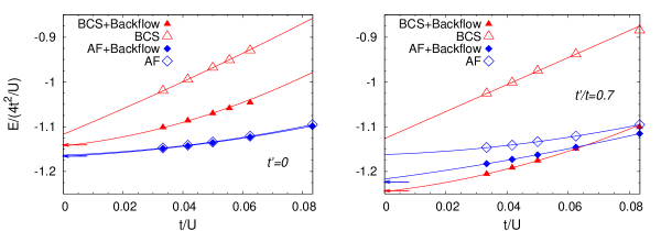
Figure 1: Variational energies per site (in unit of $J=4t^{2}/U$) for the BCS state with the Jastrow factor, with and without backflow correlations, for 98 sites and $t^{\prime}=0$ (left panel) and $t^{\prime}/t=0.7$ (right panel). The results for the wave function with antiferromagnetic order and no BCS pairing are also shown. Arrows indicate the variational results obtained by applying the full Gutzwiller projector (i.e., $g=1$) to the mean-field states for the corresponding Heisenberg models.

Thanks to backflow correlations, it is possible to obtain a correct extrapolation to the infinite-$U$ limit (i.e., to the variational energy obtained with the fully projected states $g=1$ in the Heisenberg model). On the contrary, without using backflow terms, the energy of the BCS state, even in presence of a fully optimized Jastrow factor, is few hundredths of $J=4t^{2}/U$ higher than the expected value, see Fig. 1. The importance of backflow correlations is even more evident in the frustrated case, where they are essential also for improving the accuracy of the antiferromagnetic wave function.

In order to draw the ground-state phase diagram of the $t{-}t^{\prime}$ Hubbard model, we consider three different wave functions, all with backflow correlations: One non-magnetic state $|\Psi_{BCS}\rangle$ and two antiferromagnetic states $|\Psi_{AF}\rangle$ with pitch vectors ${\bf Q}=(\pi,\pi)$ and ${\bf Q}=(\pi,0)$, relevant for small and large $t^{\prime}/t$, respectively. The variational phase diagram is reported in Fig. 2.

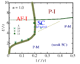
Figure 2: Left panel: Phase diagram as obtained by comparing the variational energies of different wave functions, all with backflow correlations. Right panel: Phase diagram as obtained by Yokoyama et al. by their variational approach. [5]

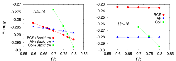
Figure 3: Variational energies for three different wave functions on the frustrated square lattice with and without backflow correlations (left and right panels, respectively). Red dots denote the energies of the spin-liquid wave function, blue triangles the energies of the magnetic state with ${\bf Q}=(\pi,\pi)$, and green squares the energies of the magnetic state with ${\bf Q}=(\pi,0)$. Data are shown for $U/t=16$ and 98 sites.

The important outcome is that without backflow terms, the energies of the spin-liquid wave function are always higher than those of the magnetically ordered states, for any value of the frustration $t^{\prime}/t$. Instead, by inserting backflow correlations, a spin-liquid phase can be stabilized at large enough $U/t$ and frustration. For example, this can be seen in Fig. 3, where we show the variational energies for the three aforementioned wave functions with and without backflow correlations, at $U/t=16$.

In order to study the metal-insulator transition, we look at the static density-density correlations $N(q)=\langle n_{-q}n_{q}\rangle$ (where $n_{q}$ is the Fourier transform of the local density $n_{i}$). Indeed, $N(q)$ shows a linear behavior for $|q|\to 0$ in the metallic phase and a quadratic behavior in the insulating region. [13] For small Coulomb repulsion and finite $t^{\prime}/t$, $N(q)$ has the linear behavior for $|q|\to 0$, typical of a conducting phase. Further, a very small superconducting parameter with $d_{x^{2}-y^{2}}$ symmetry can be stabilized (e.g., $\Delta^{ij}_{BCS}=\pm\Delta_{BCS}$ at nearest neighbors) suggesting that long-range pairing correlations, if any, are tiny. In this respect, we compare in Table 1 the optimized $\Delta_{BCS}$ when the spin-liquid wave function $|\Psi_{BCS}\rangle$ contains or not backflow correlations, for various $U/t$ and $t^{\prime}/t=0.75$. Data show that when accuracy increases, by means of backflow correlations, the BCS pairing is reduced by an order of magnitude. By increasing $U/t$, a metal-insulator transition is found and $N(q)$ acquires a quadratic behavior in the insulating phase, indicating a vanishing compressibility. In Fig. 4, we show the variational results for $N(q)$ as a function of $U/t$ for $t^{\prime}/t=0.75$. The insulator just above the transition is magnetically ordered and the variational wave function has a large $\Delta_{AF}$; the transition is likely to be first order, since the parameter $\Delta_{AF}$ has a jump across the metal-insulator transition.

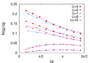
Figure 4: Variational results for $N(q)$ divided by $|q|$ for 98 (empty symbols) and 162 (full symbols) sites and $t^{\prime}/t=0.75$. The metal-insulator transition takes place between $U/t=7$ and $U/t=8$, where $N(q)$ changes from a linear to quadratic behavior for $|q|\to 0$

In the frustrated regime with $t^{\prime}/t\sim 0.7$, by further increasing $U/t$, there is a second transition to a disordered insulator. Indeed, for $U/t>14$, the energy of the BCS wave function becomes lower than the one of the antiferromagnetic state. In this respect, the key ingredient to have such an insulating behavior is the presence of a long-range Jastrow term ${\cal J}$, which turns a BCS superconductor into a Mott insulator. [13] It should be noted that the spin liquid wave function contains a superconducting gap with $d_{x^{2}-y^{2}}$ symmetry, in contrast to what was found in the infinite-$U$ limit, namely in the frustrated Heisenberg model, by a similar variational approach. [10] In fact, in the latter case, the BCS parameter contains both a term with $d_{x^{2}-y^{2}}$ symmetry and a further term with $d_{xy}$ symmetry. However, the energy gain due to the latter term is very small in the Heisenberg model (i.e., order of $0.001J$) and it is very hard to detect it when charge fluctuations are allowed (i.e., in the Hubbard model). In all cases that have been analysed, we found that the $d_{xy}$ term is not stable in the thermodynamic limit, but converges to zero as the number of lattice sites is increased.

$U/t$	$\Delta_{BCS}$ with backflow	$\Delta_{BCS}$ without backflow
7	0.042(1)	0.306(1)
6	0.031(1)	0.145(1)
4	0.012(1)	0.039(1)
2	0.002(1)	0.021(1)

Table 1: BCS pairing $\Delta_{BCS}$ for various $U/t$ in the metallic region at $t^{\prime}/t=0.75$ and 98 sites.

Wave function	Energy ($U/t=20,t^{\prime}/t=0.7$)	Energy ($U/t=8,t^{\prime}/t=0.3$)
${\cal J}|BCS\rangle$	-0.1950(1)	-0.4016(1)
${\cal J}_{HD}{\cal J}|BCS\rangle$	-0.2061(1)	-0.4180(1)
${\cal J}|BCS+\rm{Backflow}\rangle$	-0.23516(4)	-0.4879(1)
${\cal J}_{s}|AF+\rm{Backflow}\rangle$	-0.23257(3)	-0.5222(1)

Table 2: Variational energies (in unit of $t$) for three spin-liquid wave functions and for the best antiferromagnetic state with Neel order. The cluster contains 98 sites. ${\cal J}_{HD}$ is a short-range many-body Jastrow factor that has been used in Ref. [5].

We can make a direct comparison of our energies with the ones obtained by Yokoyama and collaborators, [5] who used a similar variational wave function containing a particular many-body Jastrow factor ${\cal J}_{HD}$ to correlate empty and doubly occupied sites at nearest-neighbor distances. In Table 2, we report the variational energy of the simple spin-liquid state $|\Psi_{BCS}\rangle={\cal J}|BCS\rangle$, together with the improved energies, which are obtained by adding the Jastrow term ${\cal J}_{HD}$ or by considering backflow correlations. We notice that the latter state always gives much lower energies than the one obtained with the additional Jastrow factor. In particular, let us consider the case of $U/t=8$ and $t^{\prime}/t=0.3$, which should be magnetically ordered according to our calculations and disordered according to Ref. [5] (see Fig. 2). In this case, even though our spin-liquid state has a much better energy than the one with ${\cal J}_{HD}$, the best wave function has Neel order, indicating that the stability region of antiferromagnetism is larger than what predicted by Yokoyama and collaborators. [5]

To conclude, we compare the variational energies with the ones obtained by the Green’s function Monte Carlo approach, implemented within the Fixed Node (FN) approximation. In brief, the FN method allows one to filter out the high-energy components of a given state and to find the best variational state with the same nodes of the starting one. [20] On the lattice, the FN method can be defined as follows: Starting from the original Hamiltonian ${\cal H}$, we define an effective Hamiltonian by adding a perturbation $O$:

$${\cal H}^{eff}={\cal H}+O.$$ (8)

The operator $O$ is defined through its matrix elements and depends upon a given guiding function $|\Psi\rangle$, that is for instance the variational state itself

$$O_{x^{\prime},x}=\left\{\begin{array}[]{ll}-{\cal H}_{x^{\prime},x}&{\rm if}\;s_{x^{\prime},x}=\Psi_{x^{\prime}}{\cal H}_{x^{\prime},x}\Psi_{x}>0\\ \sum_{y,s_{y,x}>0}{\cal H}_{y,x}\frac{\Psi_{y}}{\Psi_{x}}&{\rm for}\;x^{\prime}=x,\end{array}\right.$$

where $\Psi_{x}=\langle x|\Psi\rangle$, $|x\rangle$ being a generic many-body configuration. The most important property of this effective Hamiltonian is that its ground state $|\Psi_{0}\rangle$ can be efficiently computed by using the Green’s function Monte Carlo technique, [21, 22] which allows one to sample the distribution $\Pi_{x}\propto\langle x|\Psi\rangle\langle x|\Psi_{0}\rangle$ by means of a statistical implementation of the power method: $\Pi\propto\lim_{n\to\infty}G^{n}\Pi^{0}$, where $\Pi^{0}$ is a starting distribution and $G_{x^{\prime},x}=\Psi_{x^{\prime}}(\Lambda\delta_{x^{\prime},x}-{\cal H}^{eff}_{x^{\prime},x})/\Psi_{x}$ is the so-called Green’s function, defined with a large or even infinite positive constant $\Lambda$, $\delta_{x^{\prime},x}$ being the Kronecker symbol. The statistical method is very efficient since in this case all the matrix elements of $G$ are non-negative and, therefore, it can represent a transition probability in configuration space, apart for a normalization factor $b_{x}=\sum_{x^{\prime}}G_{x^{\prime},x}$. In this case, it follows immediately that the asymptotic distribution $\Pi$ is also positive and, therefore, we arrive at the important conclusion that the ground state of ${\cal H}^{eff}$ has the same signs of the chosen guiding function (i.e., the best variational state).

In Fig. 5, we show the variational energies per site (with backflow correlations) and the FN ones for $U/t=16$ on a 98-site lattice. The small energy difference between the pure variational energies and the FN ones demonstrates the accuracy of the backflow states. Notice that $|\Psi_{AF}\rangle$ and $|\Psi_{BCS}\rangle$ have different nodal surfaces, implying different FN energies.

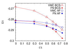
Figure 5: Comparison between the variational (VMC) energies per site (with backflow correlations) and the FN ones. Data are shown for $U/t=16$ and 98 sites.

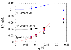
Figure 6: Variational (empty symbols) and FN (full symbols) results for $S(\pi,\pi)/N$, for $N=18$, $50$, $98$, and $162$. All the calculations have been done by using the projected BCS wave function; $U/t=16$ and $t^{\prime}/t=0$ (triangles), $U/t=24$ and $t^{\prime}/t=0.7$ (circles) and $U/t=8$ and $t^{\prime}/t=0.75$ (squares). Lines are guides to the eye.

In order to verify the magnetic properties obtained within the variational approach, we can consider the static spin-spin correlations $S(q)=\langle S^{z}_{q}S^{z}_{-q}\rangle$, where $S^{z}_{q}$ is the Fourier transform of the local spin $S^{z}_{i}$. Although the FN approach may break the SU(2) spin symmetry, favoring a spin alignment along the $z$ axis, $S(q)$ is particularly simple to evaluate within this approach, [20] and it gives important insights into the magnetic properties of the ground state. In Fig. 6, we report the comparison between the variational and the FN results by using the non-magnetic state $|\Psi_{BCS}\rangle$. Remarkably, in the unfrustrated case, where antiferromagnetic order takes place, the FN approach is able to increase spin-spin correlations at ${\bf Q}=(\pi,\pi)$, even by considering the non-magnetic wave function to fix the nodes. In this case, the FN results are qualitatively different from the pure variational ones, which indicate no magnetic order in the thermodynamic limit. A finite value of the magnetization is also plausible in the insulating region just above the metallic phase at strong frustration (i.e., $t^{\prime}/t\sim 0.75$), confirming our variational calculations. On the contrary, by increasing electron correlation, FN results change only slightly the variational value of $S(\pi,\pi)$, indicating the stability of the disordered state. Therefore, the FN results confirm that a spin liquid region can be stabilized only at large enough $U/t$, while the insulator close to the metallic region is magnetically ordered.

In summary, the backflow wave functions represent simple and useful generalizations of standard projected states, which are used to describe strongly correlated materials. They are highly accurate and may give important insights into the ground-state properties of frustrated models with itinerant electrons.

We acknowledge CNR-INFM for partial support.

References

- [1] H.Q. Lin and J.E. Hirsch, Phys. Rev. B 35, 3359 (1987).
- [2] T. Kashima and M. Imada, J. Phys. Soc. Jpn. 70, 3052 (2001).
- [3] H. Morita, S. Watanabe, and M. Imada, J. Phys. Soc. Jpn. 71, 2109 (2002).
- [4] T. Mizusaki and M. Imada, Phys. Rev. B 74, 014421 (2006).
- [5] H. Yokoyama, M. Ogata, and Y. Tanaka, J. Phys. Soc. Jpn. 75, 114706 (2006).
- [6] A.H. Nevidomskyy, C. Scheiber, D. Senechal, and A.-M.S. Tremblay, Phys. Rev. B 77, 064427 (2008); see also, S.R. Hassan, B. Davoudi, B. Kyung, and A.-M.S. Tremblay, Phys. Rev. B 77, 094501 (2008).
- [7] L.F. Tocchio, F. Becca, A. Parola, and S. Sorella, Phys. Rev. B 78, 041101(R) (2008).
- [8] F. Becca, M. Capone, and S. Sorella, Phys. Rev. B 62, 12700 (2000).
- [9] P.W. Anderson, Science 235, 1196 (1987).
- [10] L. Capriotti, F. Becca, A. Parola, and S. Sorella, Phys. Rev. Lett. 87, 097201 (2001).
- [11] S. Yunoki and S. Sorella, Phys. Rev. B 74, 014408 (2006).
- [12] H. Yokoyama and H. Shiba, J. Phys. Soc. Jpn. 56, 1490 (1987).
- [13] M. Capello, F. Becca, M. Fabrizio, S. Sorella, and E. Tosatti, Phys. Rev. Lett. 94, 026406 (2005).
- [14] R.P. Feynman and M. Cohen, Phys. Rev. 102, 1189 (1956).
- [15] M.A. Lee, K.E. Schmidt, M.H. Kalos, and G.V. Chester, Phys. Rev. Lett. 46, 728 (1981).
- [16] K.E. Schmidt, M.A. Lee, M.H. Kalos, and G.V. Chester, Phys. Rev. Lett. 47, 807 (1981).
- [17] Y. Kwon, D.M. Ceperley, and R.M. Martin, Phys. Rev. B 48, 12037 (1993).
- [18] Y. Kwon, D.M. Ceperley, and R.M. Martin, Phys. Rev. B 58, 6800 (1998).
- [19] M. Holzmann, D.M. Ceperley, C. Pierleoni, and K. Esler, Phys. Rev. E 68, 046707 (2003).
- [20] D.F.B. ten Haaf, H.J.M. van Bemmel, J.M.J. van Leeuwen, W. van Saarloos, and D.M. Ceperley, Phys. Rev. B 51, 13039 (1995).
- [21] N. Trivedi and D.M. Ceperley, Phys. Rev. B 41, 4552 (1990).
- [22] M. Calandra and S. Sorella, Phys. Rev. B 57, 11446 (1998).