Slicing planar grid diagrams: a gentle introduction to bordered Heegaard Floer homology

Abstract.

We describe some of the algebra underlying the decomposition of planar grid diagrams. This provides a useful toy model for an extension of Heegaard Floer homology to 3-manifolds with parametrized boundary. This paper is meant to serve as a gentle introduction to the subject, and does not itself have immediate topological applications.

1. Introduction

The Heegaard Floer homology groups of Ozsváth and Szabó are defined in terms of holomorphic curves in Heegaard diagrams. In [7], Heegaard Floer homology is extended to three-manifolds with (parameterized) boundary, by studying holomorphic curves in pieces of Heegaard diagrams. The resulting invariant, bordered Heegaard Floer homology, has the following form. To an oriented surface $F$ (together with an appropriate Morse function on $F$), bordered Heegaard Floer associates a differential graded algebra $\mathcal{A}(F)$. To a three-manifold $Y$ together with a homeomorphism $F\to\partial Y$, bordered Heegaard Floer associates a right ($\mathcal{A}_{\infty})$ module $\widehat{\mathit{CFA}}(Y)$ over $\mathcal{A}(F)$ and a left (differential graded) module $\widehat{\mathit{CFD}}(Y)$ over $\mathcal{A}(-F)$. (Here, $-F$ denotes $F$ with its orientation reversed.) These modules, which are well-defined up to homotopy equivalence, relate to the closed Heegaard Floer homology group $\widehat{\mathit{HF}}$ via the following pairing theorem:

Theorem 1 ([7]).

Suppose that $Y=Y_{1}\cup_{F}Y_{2}$. Then $\widehat{\mathit{CF}}(Y)\simeq\widehat{\mathit{CFA}}(Y_{1})\mathop{\widetilde{\otimes}}\nolimits_{\mathcal{A}(F)}\widehat{\mathit{CFD}}(Y_{2})$.

(Recall that $\widehat{\mathit{CF}}(Y)$ is the chain complex underlying the Floer homology group $\widehat{\mathit{HF}}(Y)$. The notation $\mathop{\widetilde{\otimes}}\nolimits$ denotes the derived tensor product, and the symbol $\simeq$ denotes quasi-isomorphism.)

The definitions of the invariants $\widehat{\mathit{CFA}}$ and $\widehat{\mathit{CFD}}$ are, unfortunately, somewhat involved. There are two kinds of complications which obscure the basic ideas involved:

• Analytic complications. The definitions of the invariants $\widehat{\mathit{CFA}}$ and $\widehat{\mathit{CFD}}$ involve counting pseudo-holomorphic curves. In spite of much progress over the last decades, holomorphic curve techniques remain somewhat technical, and often require seemingly unnatural contortions. To make matters worse, the analytic set up is, by necessity, somewhat nonstandard; in particular, it involves counting curves in a manifold with “two kinds of infinities.”

• Algebraic complications. The invariant $\widehat{\mathit{CFA}}$ is, in general, not an honest module but only an $\mathcal{A}_{\infty}$-module. While the subject of $\mathcal{A}_{\infty}$ algebra is increasingly mainstream, it still adds a layer of obfuscation to the study of bordered Heegaard Floer homology. Further exacerbating the situation is a somewhat novel kind of grading.

In developing bordered Heegaard Floer homology we found it useful to study a toy model, in terms of planar grid diagrams, in which these complications are absent. It is the aim of the present paper to present this toy model. We hope that doing so will make the definition of bordered Heegaard Floer homology in [7] more palatable.

We emphasize up front that the main objects of study in this paper do not give topological invariants. Still, the algebra involved is reminiscent of well-known objects from representation theory—in particular, the nilCoxeter algebra—so this paper may be of further interest.

Throughout this paper, $\mathbb{F}$ will denote the field with two elements and $\mathbb{A}$ will denote $\mathbb{F}[U_{1},\dots,U_{N}]$ (for whichever $N$ is in play at the time).

Acknowledgements. The first author thanks the organizers of the Gökova Geometry/Topology Conference for inviting him to participate in this stimulating event. He also thanks C. Douglas for interesting conversations in the summer of 2006. The authors also thank M. Khovanov for pointing out the relationship of the algebra $\mathcal{A}$ with the nilCoxeter algebra.

2. Background on knot Floer homology and grid diagrams

We start by recalling the combinatorial definition of Manolescu-Ozsváth-Sarkar [8] of the knot Floer homology groups.

Let $K$ be an oriented knot in $S^{3}$. Choose a knot diagram $D$ for $K$ such that

• $D$ is composed entirely of horizontal and vertical segments,

• no two horizontal segments of $D$ have the same $y$-coordinate, and no two vertical segments of $D$ have the same $x$-coordinate, and

• at each crossing, the vertical segment crosses over the horizontal segment.

(Every knot admits such a diagram; see Figure 1.) The only data in such a diagram are the endpoints of the segments, which we record by placing $X$’s and $O$’s at these endpoints, alternately around the knot, and so that the knot is oriented from $X$ to $O$ along vertical segments. Notice that no two $X$’s (respectively $O$’s) lie on the same horizontal or vertical line.

Let $\mathbb{X}=\{X_{i}\}_{i=1}^{N}$ and $\mathbb{O}=\{O_{i}\}_{i=1}^{N}$ denote the set of $X$’s and $O$’s, respectively. Up to isotopy of the knot (and renumbering of the $X_{i}$), we may assume that the coordinates of $X_{i}$ are $\left(i-\frac{1}{2},\sigma_{\mathbb{X}}(i)-\frac{1}{2}\right)$ for some permutation $\sigma_{\mathbb{X}}\in S_{N}$. Then (after renumbering), the coordinates of $O_{i}$ are $\left(i-\frac{1}{2},\sigma_{\mathbb{O}}(i)-\frac{1}{2}\right)$ for some permutation $\sigma_{\mathbb{O}}\in S_{N}$. The data $(\mathbb{R}^{2},\mathbb{X},\mathbb{O})$ is a planar grid diagram for the knot $K$.

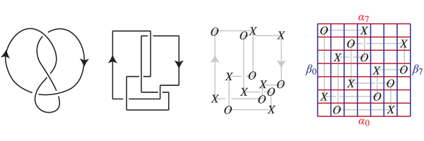
Figure 1. Representing a knot by a grid diagram. Starting with a knot diagram $D$, one approximates $D$ using horizontal and vertical segments, so that crossings are always vertical over horizontal. Perturb the result so that no segments lie on the same horizontal or vertical line, and mark the endpoints alternately with $X$’s and $O$’s. The data of the knot is entirely encoded in these $X$’s and $O$’s, which we can see as sitting in the middle of squares on a piece of graph paper.

We can also view $\mathbb{X}$ and $\mathbb{O}$ as subsets of the torus $T=\mathbb{R}^{2}/\langle(N,0),(0,N)\rangle.$ The data $(T,\mathbb{X},\mathbb{O})$ is a toroidal grid diagram for the knot $K$. It is easy to recover the knot $K$ (up to isotopy) from the toroidal grid diagram $(T,\mathbb{X},\mathbb{O})$. We call the process of passing from a planar grid diagram to a toroidal grid diagram wrapping. The inverse operation of passing from a toroidal grid diagram to a planar grid diagram, which depends on a choice of two circles in $T$, we call unwrapping.

The $N+1$ lines $\alpha_{i}=\{y=i\}\subset\mathbb{R}^{2}$, $i=0,\dots,N$, descend to $N$ disjoint circles $\overline{\alpha}_{i}$ in the torus $T$, with $\overline{\alpha}_{0}=\overline{\alpha}_{N}$. Similarly, the $N+1$ lines $\beta_{i}=\{x=i\}\subset\mathbb{R}^{2}$, $i=0,\dots,N$, descend to $N$ disjoint circles $\overline{\beta}_{i}$ in $T$. Notice that each $\alpha_{j}$ (respectively $\overline{\alpha}_{j}$) intersects each $\beta_{i}$ (respectively $\overline{\beta}_{j}$) in a single point. Set ${\boldsymbol{\alpha}}=\bigcup_{i=0}^{N}\alpha_{i}$, $\overline{\boldsymbol{\alpha}}=\bigcup_{i=1}^{N}\overline{\alpha}_{i}$, ${\boldsymbol{\beta}}=\bigcup_{i=0}^{N}\beta_{i}$ and $\overline{\boldsymbol{\beta}}=\bigcup_{i=1}^{N}\overline{\beta}_{i}$. We view the $\overline{\alpha}_{i}$ as “horizontal” and the $\overline{\beta}_{i}$ as “vertical”. This means that components of $T\setminus\left(\overline{\boldsymbol{\alpha}}\cup\overline{\boldsymbol{\beta}}\right)$ (little rectangles) have, for instance, lower left corners, lower right corners, and so on.

We define the knot Floer chain complex $\mathit{CFK}^{-}(K)$ as follows. Let $\mathbb{A}=\mathbb{F}[U_{1},\dots,U_{N}]$. By a toroidal generator we mean an $N$-tuple of points $\mathbf{x}=\{x_{i}\in\overline{\alpha}_{\sigma(i)}\cap\overline{\beta}_{i}\}$, one on each $\overline{\alpha}$-circle and one on each $\overline{\beta}$-circle. Generators, then, are in bijection with the permutation group $S_{N}$—but this bijection depends on a choice of unwrapping. Let $\mathfrak{S}(T,\mathbb{X},\mathbb{O})$ denote the set of generators. The knot Floer complex $\mathit{CFK}^{-}(K)$ is freely generated over $\mathbb{A}$ by $\mathfrak{S}(T,\mathbb{X},\mathbb{O})$.

For two generators $\mathbf{x}=\{x_{i}\}$ and $\mathbf{y}=\{y_{i}\}$, we define a set $\overline{\operatorname{Rect}}(\mathbf{x},\mathbf{y})$. The set $\overline{\operatorname{Rect}}(\mathbf{x},\mathbf{y})$ is empty unless all but two of the $x_{i}$ agree with corresponding $y_{i}$. In that case, let $\{i,j\}=\{k\mid x_{k}\neq y_{k}\}$; then $\overline{\operatorname{Rect}}(\mathbf{x},\mathbf{y})$ is the set of embedded rectangles $R$ in $T$ with boundary on ${\boldsymbol{\alpha}}\cup{\boldsymbol{\beta}}$, and such that $x_{i}$ and $x_{j}$ are the lower-left and upper-right corners of $R$ (in either order), and $y_{i}$ and $y_{j}$ are the upper-left and lower-right corners of $R$ (in either order). (Consequently, $\overline{\operatorname{Rect}}(\mathbf{x},\mathbf{y})$ always has either zero or two elements.) Call a rectangle $R\in\overline{\operatorname{Rect}}(\mathbf{x},\mathbf{y})$ empty if the interior of $R$ contains no point in $\mathbf{x}$, and define $\overline{\operatorname{Rect}}^{\circ}(\mathbf{x},\mathbf{y})$ to be the set of empty rectangles in $\overline{\operatorname{Rect}}(\mathbf{x},\mathbf{y})$. Given a rectangle $R$, define $O_{i}(R)$ to be $1$ if $O_{i}$ lies in the interior of $R_{i}$ and zero otherwise. Define $X_{i}(R)$ similarly, and set $\mathbb{O}(R)=\sum_{i=1}^{N}O_{i}(R)$ and $\mathbb{X}(R)=\sum_{i=1}^{N}X_{i}(R)$. Set $U(R)=\prod_{i}U_{i}^{O_{i}(R)}$.

Now, define

(2.1) $$\partial\mathbf{x}=\sum_{\mathbf{y}\in\mathfrak{S}(T,\mathbb{X},\mathbb{O})}\sum_{\begin{subarray}{c}R\in\overline{\operatorname{Rect}}^{\circ}(\mathbf{x},\mathbf{y})\\ \mathbb{X}(R)=0\end{subarray}}U(R)\cdot\mathbf{y}.$$

Lemma 2.2.

Formula (2.1) defines a differential, i.e., $\partial^{2}=0$.

This is not hard to prove [9, Proposition 2.8]. See Figure 2 for some of the cases.

By composing rectangles, we get more complicated regions in $T$, called domains. By a domain connecting $\mathbf{x}$ to $\mathbf{y}$ we mean a cellular two-chain $B$ in $(T,\overline{\boldsymbol{\alpha}}\cup\overline{\boldsymbol{\beta}})$ with the following property. Let $\partial_{\alpha}B$ denote the intersection of $\partial B$ with ${\boldsymbol{\alpha}}$. Then we require $\partial(\partial_{\alpha}B)=\mathbf{y}-\mathbf{x}$. We can define $O_{i}(B)$, $X_{i}(B)$, $\mathbb{O}(B)$, $\mathbb{X}(B)$, and $U(B)$ in the same way as for rectangles.

There are two $\mathbb{Z}$-gradings on $\mathit{CFK}^{-}(K)$, the Maslov or homological grading, denoted $\mu$, and the Alexander grading, denoted $A$. These have the property that $\partial$ preserves $A$ and lowers $\mu$ by $1$. We give the combinatorial characterization of $A$ and $\mu$ from [9], up to an overall shift. First, some notation. Given sets $E$ and $F$ in $\mathbb{R}^{2}$, let $\mathcal{I}(E,F)$ denote the number of pairs $(e,f)\in E\times F$ such that $e$ lies to the lower left of $f$ (i.e., the number of pairs $e=(e_{1},e_{2})\in\mathbb{R}^{2}$ and $f=(f_{1},f_{2})\in\mathbb{R}^{2}$, such that $e_{1}<f_{1}$ and $e_{2}<f_{2}$).

Now, fix an unwrapping $(\mathbb{R}^{2},\mathbb{X},\mathbb{O})$ of the diagram $(T,\mathbb{X},\mathbb{O})$, so a generator $\mathbf{x}\in\mathfrak{S}(T,\mathbb{X},\mathbb{O})$ corresponds to a $N$-tuple of points $u(\mathbf{x})$ in $\mathbb{R}^{2}$. Then, for some constants $C_{A}$ and $C_{\mu}$ depending on the diagram and the unwrapping (but not on $\mathbf{x}$),

$$A(\mathbf{x}) =\mathcal{I}(\mathbb{X},\mathbf{x})-\mathcal{I}(\mathbb{O},\mathbf{x})+C_{A}$$

$$\mu(\mathbf{x}) =\mathcal{I}(\mathbf{x},\mathbf{x})-2\mathcal{I}(\mathbb{O},\mathbf{x})+C_{\mu},$$

cf. [9, Formulas (1) and (2)], bearing in mind that $I(\mathbb{X},\mathbf{x})$ differs from $I(\mathbf{x},\mathbb{X})$ by a constant. Together with the property that $A(U_{i})=-1$ and $\mu(U_{i})=-2$ this characterizes $A$ and $\mu$ up to overall additive constants.

A fundamental result of Manolescu-Ozsváth-Sarkar [8] states that the complex $\mathit{CFK}^{-}(K)$ defined above is bi-graded homotopy equivalent to the complex $\mathit{CFK}^{-}(K)$ defined by Ozsváth and Szabó [10] and also by Rasmussen [11]. It follows, in particular, that the homotopy type of $\mathit{CFK}^{-}(K)$ is independent of the toroidal grid diagram for $K$. The fact that the homotopy type of $\mathit{CFK}^{-}(K)$ depends only on the knot $K$ can also be proved combinatorially [9].

2.1. Planar Floer Homology

In this paper we will study a modification of the grid diagram construction of $\mathit{CFK}^{-}$, which we call the planar Floer homology and denote $\mathit{CP}^{-}$, obtained by replacing toroidal grid diagrams by planar grid diagrams throughout the definition of $\mathit{CFK}^{-}$. In the planar setting, when we have $N$ different $X$’s we will have $N+1$ different $\alpha$- (respectively $\beta$-) lines: we view the process of wrapping the diagram as identifying $\alpha_{0}$ with $\alpha_{N}$, and $\beta_{0}$ with $\beta_{N}$. Thus, a generator over $\mathbb{A}$ of the complex $\mathit{CP}^{-}(\mathbb{X},\mathbb{O})$ is an $(N+1)$-tuple of points $\mathbf{x}=\{x_{i}\in\alpha_{\sigma(i)}\cap\beta_{i}\}_{i=0}^{N}$. The set $\mathfrak{S}(\mathbb{R}^{2},\mathbb{X},\mathbb{O})$ is in canonical bijection with the symmetric group $S_{N+1}$.

Given generators $\mathbf{x}$ and $\mathbf{y}$ in $\mathfrak{S}(\mathbb{R}^{2},\mathbb{X},\mathbb{O})$, let $\operatorname{Rect}^{\circ}(\mathbf{x},\mathbf{y})$ denote the set of empty rectangles in $\mathbb{R}^{2}$ connecting $\mathbf{x}$ to $\mathbf{y}$; for each $\mathbf{x}$ and $\mathbf{y}$ the set $\operatorname{Rect}^{\circ}(\mathbf{x},\mathbf{y})$ is either empty or has a single element. The differential on $\mathit{CP}^{-}$ is defined analogously to Formula (2.1):

(2.3) $$\partial\mathbf{x}=\sum_{\mathbf{y}\in\mathfrak{S}(\mathbb{R}^{2},\mathbb{X},\mathbb{O})}\sum_{\begin{subarray}{c}R\in\operatorname{Rect}^{\circ}(\mathbf{x},\mathbf{y})\\ \mathbb{X}(R)=0\end{subarray}}U(R)\cdot\mathbf{y}.$$

Lemma 2.4.

Formula (2.3) defines a differential, i.e., $\partial^{2}=0$.

The proof, which is a strict sub-proof of the proof for toroidal grid diagrams, is illustrated in Figure 2.

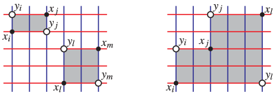
Figure 2. Illustration of why $\partial^{2}=0$ for planar Floer homology. Left: The contributions to the coefficient of $\mathbf{y}$ from taking the two shaded rectangles in the two orders cancel. Right: This “L”-shaped domain can be decomposed into two rectangles in two different ways, by making either a horizontal cut or a vertical cut. These two contributions cancel.

The complex $\mathit{CP}^{-}(\mathbb{X},\mathbb{O})$ has Alexander and Maslov gradings $A$ and $\mu$, defined exactly as they were for $\mathit{CFK}^{-}(K)$. We fix the additive constants by setting

$$A(\mathbf{x}) =\mathcal{I}(\mathbb{X},\mathbf{x})-\mathcal{I}(\mathbb{O},\mathbf{x})$$

$$\mu(\mathbf{x}) =\mathcal{I}(\mathbf{x},\mathbf{x})-2\mathcal{I}(\mathbb{O},\mathbf{x}).$$

Warning: The homotopy type of the complex $\mathit{CP}^{-}(\mathbb{X},\mathbb{O})$ is not an invariant of the underlying knot $K$. This is illustrated in Example 2.5. The results of this paper, thus, do not directly give new topological invariants.

Example 2.5.

Consider the planar grid diagrams for the unknot shown in Figure 3. The diagram on the left has $N=1$. The complex has two generators over $\mathbb{F}[U_{1}]$, which we label with the permutations $[\begin{array}[]{@{}*{10}{c@{\,}}}1&2\end{array}\!]$ and $[\begin{array}[]{@{}*{10}{c@{\,}}}2&1\end{array}\!]$ in one-line notation. (Here the one-line notation $[\begin{array}[]{@{}*{10}{c@{\,}}}2&3&1\end{array}\!]$, for instance, means the permutation $\{1\mapsto 2,2\mapsto 3,3\mapsto 1\}$.) The differential is trivial, so the homology of the complex is $\mathbb{F}[U_{1}]^{\oplus 2}$.

The diagram on the right has $N=2$. The complex has six generators. The differential is given by

$$\partial[\begin{array}[]{@{}*{10}{c@{\,}}}2&3&1\end{array}\!] =U_{1}[\begin{array}[]{@{}*{10}{c@{\,}}}3&2&1\end{array}\!]$$

$$\partial[\begin{array}[]{@{}*{10}{c@{\,}}}3&1&2\end{array}\!] =U_{2}[\begin{array}[]{@{}*{10}{c@{\,}}}3&2&1\end{array}\!]$$

$$\partial[\begin{array}[]{@{}*{10}{c@{\,}}}3&2&1\end{array}\!] =\partial[\begin{array}[]{@{}*{10}{c@{\,}}}1&2&3\end{array}\!]=\partial[\begin{array}[]{@{}*{10}{c@{\,}}}1&3&2\end{array}\!]=\partial[\begin{array}[]{@{}*{10}{c@{\,}}}2&1&3\end{array}\!]=0.$$

The homology of the complex is

$$\mathbb{F}\left\langle[\begin{array}[]{@{}*{10}{c@{\,}}}3&2&1\end{array}\!]\right\rangle\oplus\mathbb{F}[U_{1},U_{2}]\left\langle[\begin{array}[]{@{}*{10}{c@{\,}}}1&2&3\end{array}\!],[\begin{array}[]{@{}*{10}{c@{\,}}}1&3&2\end{array}\!],[\begin{array}[]{@{}*{10}{c@{\,}}}2&1&3\end{array}\!],U_{2}[\begin{array}[]{@{}*{10}{c@{\,}}}2&3&1\end{array}\!]+U_{1}[\begin{array}[]{@{}*{10}{c@{\,}}}3&1&2\end{array}\!]\right\rangle.$$

This is certainly not the same as $\mathbb{F}[U_{1}]^{\oplus 2}$.

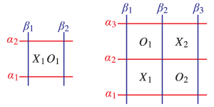
Figure 3. Planar grid diagrams for the unknot. Left: a diagram with $N=1$. Right: a diagram with $N=2$. The corresponding planar Floer complexes are not homotopy equivalent (Example 2.5).

3. Slicing planar grid diagrams

Fix a planar grid diagram $\mathcal{H}=(\mathbb{R}^{2},\mathbb{X},\mathbb{O})$. The goal of this paper is to compute the complex $\mathit{CP}^{-}(\mathcal{H})$ by cutting the diagram vertically into pieces. (For now, we consider only cutting $\mathcal{H}$ into two pieces; we will consider more general cuttings in Section 9.1.) We want to associate something (ultimately, it will be a differential module) to each side, and something (ultimately, it will be a differential graded algebra) to the interface between the two sides. We want these to contain enough information to reconstruct $\mathit{CP}^{-}(\mathcal{H})$—but as little information as possible beyond that, so as to be computable.

So, let $Z$ be the vertical line $\{x=k-1/4\}$ and consider what each side of $Z$ looks like. To the left of $Z$ we have $k$ vertical lines $\beta_{0},\dots,\beta_{k-1}$, as well as two injective maps $\mathbb{X}^{A}\colon\{1,\dots,k\}\to\{1,\dots,N\}$ and $\mathbb{O}^{A}\colon\{1,\dots,k\}\to\{1,\dots,N\}$. Similarly, to the right of $Z$ we have $N+1-k$ vertical lines $\beta_{k},\dots,\beta_{N}$, as well as two injective maps $\mathbb{X}^{D}\colon\{k+1,\dots,N\}\to\{1,\dots,N\}$ and $\mathbb{O}^{D}\colon\{k+1,\dots,N\}\to\{1,\dots,N\}$. There are also $N+1$ $\alpha$-lines, which intersect both sides of the diagram. Finally, at the interface $Z$ we see $N+1$ points $\{(i,k-1/4)\}_{i=0}^{N}$ where the $\alpha_{i}$ intersect $Z$. See Figure 4.

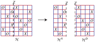
Figure 4. Cutting a planar grid diagram. The resulting diagrams $\mathcal{H}^{A}$ and $\mathcal{H}^{D}$ have $N=7$ and $k=3$.

Let $H^{A}$ denote the half-plane to the left of $Z$, and $H^{D}$ the half-plane to the right of $Z$. We will call the data $\mathcal{H}^{A}=(H^{A},\mathbb{X}^{A},\mathbb{O}^{A})$ or $\mathcal{H}^{D}=(H^{D},\mathbb{X}^{D},\mathbb{O}^{D})$ a partial planar grid diagram. If we view $Z$ as oriented upwards then there is a distinction between $\mathcal{H}^{A}$ and $\mathcal{H}^{D}$: for $\mathcal{H}^{A}$ the induced orientation of $Z$ agrees with the given one, while for $\mathcal{H}^{D}$ the induced orientation differs. We will call the first case “type $A$” and the second case “type $D$.” We say that $\mathcal{H}^{A}$ has height $N+1$ and width $k$, and $\mathcal{H}^{D}$ has height $N+1$ and width $N+1-k$.

Finally, a generator $\mathbf{x}=\{x_{i}\}_{i=0}^{N}$ corresponds to $k$ points $\mathbf{x}^{A}=\{x_{i}\in\alpha_{\sigma^{A}(i)}\cap\beta_{i}\}_{i=0}^{k-1}$ to the left of $Z$ and $N+1-k$ points $\mathbf{x}^{D}=\{x_{i}\in\alpha_{\sigma^{D}(i)}\cap\beta_{i}\}_{i=k}^{N}$ to the right of $Z$. Here, $\sigma^{A}$ is an injection $\{0,\dots,k-1\}\to\{0,\dots,N\}$ and $\sigma^{D}$ is an injection $\{k,\dots,N\}\to\{0,\dots,N\}$. For use later, let $\mathfrak{S}(\mathcal{H}^{A})$ denote the set of $k$-tuples $\mathbf{x}^{A}=\{x_{i}\in\alpha_{\sigma^{A}(i)}\cap\beta_{i}\}_{i=0}^{k-1}$ where $\sigma^{A}$ is an injection $\{0,\dots,k-1\}\to\{0,\dots,N\}$. Let $\mathfrak{S}(\mathcal{H}^{D})$ denote the set of $(N+1-k)$-tuples $\mathbf{x}^{D}=\{x_{i}\in\alpha_{\sigma^{D}(i)}\cap\beta_{i}\}_{i=k}^{N}$ where $\sigma^{D}$ is an injection $\{k,\dots,N\}\to\{0,\dots,N\}$.

4. Motivating the answer

The purpose of this section is to motivate the answers which will be described in later sections; thus, it can be skipped by the impatient reader without sacrificing mathematical content.

We want to associate some kind of object, which with hindsight we will call $\mathit{CPA}^{-}(\mathcal{H}^{A})$ to $\mathcal{H}^{A}$, and some other kind of object $\mathit{CPD}^{-}(\mathcal{H}^{D})$ to $\mathcal{H}^{D}$. These should be objects in some (algebraic) categories $\mathcal{C}^{A}$ and $\mathcal{C}^{D}$ associated to the interface $Z$ (together perhaps with a little additional data). We would also like a pairing map $P$ from $\mathcal{C}^{A}\times\mathcal{C}^{D}$ to $\mathcal{D}^{b}(\mathbb{A}-\mathsf{Mod})$, the derived category of complexes over the ground ring $\mathbb{A}$, so that $\mathit{CP}^{-}(\mathcal{H})=P(\mathcal{H}^{A},\mathcal{H}^{D})$. The (derived) category of chain complexes of (right/left) $\mathcal{A}$-modules for any $\mathbb{A}$-algebra $\mathcal{A}$ admit such a pairing map, so this seems like a reasonable example to keep in mind. (That is also how the story goes in Khovanov homology [3], which is encouraging.)

Since a generator $\mathbf{x}$ of $\mathit{CP}^{-}(\mathcal{H})$ decomposes as a pair $(\mathbf{x}^{A},\mathbf{x}^{D})$, it seems reasonable that $\mathit{CPA}^{-}(\mathcal{H}^{A})$ would be generated—in some sense to be determined—by $\mathfrak{S}(\mathcal{H}^{A})$ and that $\mathit{CPD}^{-}(\mathcal{H}^{D})$ would be generated by $\mathfrak{S}(\mathcal{H}^{D})$.

Not every pair $(\mathbf{x}^{A},\mathbf{x}^{D})\in\mathfrak{S}(\mathcal{H}^{A})\times\mathfrak{S}(\mathcal{H}^{D})$ corresponds to a generator in $\mathfrak{S}(\mathcal{H})$: the necessary and sufficient condition is that the images of the injections $\sigma^{A}$ and $\sigma^{D}$ be disjoint. It seems reasonable that our putative $\mathcal{A}$ would remember this—that if $\sigma^{A}_{1}$ and $\sigma^{A}_{2}$ have different images then corresponding generators $\mathbf{x}_{1}^{A}$ and $\mathbf{x}_{2}^{A}$ would “live over” different “objects” in $\mathcal{A}$. In the language of differential graded categories (see, e.g., [2]), this makes sense; for algebras this can be encoded via idempotents. That is, suppose $\mathcal{A}$ has $\binom{N+1}{k}$ different primitive idempotents $I_{S}$, one for each $k$-element subset $S$ of $\{0,\dots,N\}$. Then we could say $\mathbf{x}^{A}I_{S}=\mathbf{x}^{A}$ if and only if $S=\mathrm{Im}(\sigma^{A})$, and $I_{S}\mathbf{x}^{D}=\mathbf{x}^{D}$ if and only if $S\cap\mathrm{Im}(\sigma^{D})=\emptyset$; otherwise these products are $0$. It then follows that an expression of the form $\mathbf{x}^{A}\otimes_{\mathcal{A}}\mathbf{x}^{D}$ is nonzero if and only if $(\mathbf{x}^{A},\mathbf{x}^{D})$ actually corresponds to a generator in $\mathfrak{S}(\mathcal{H})$. We will write $S(\mathbf{x}^{A})$ to denote $\mathrm{Im}(\sigma^{A})$, and $S(\mathbf{x}^{D})$ to denote $\{0,\dots,N\}\setminus\mathrm{Im}(\sigma^{D})$.

There are three kinds of rectangles which contribute to the differential on $\mathit{CP}^{-}(\mathcal{H})$:

• Rectangles contained entirely in $\mathcal{H}^{A}$. It seems reasonable that these should contribute to a differential on $\mathit{CPA}^{-}(\mathcal{H}^{A})$, and there is an obvious way for them to do so.

• Rectangles contained entirely in $\mathcal{H}^{D}$. Again, it seems reasonable to let these contribute to a differential on $\mathit{CPD}^{-}(\mathcal{H}^{D})$.

• Rectangles which cross through the interface $Z$. It is somewhat less clear how to count these.

Let $R$ be a rectangle crossing through $Z$. Each of $\mathit{CPA}^{-}(\mathcal{H}^{A})$ and $\mathit{CPD}^{-}(\mathcal{H}^{D})$ see $Z$ as a half strip, and these half strips should somehow be involved in the definitions of $\mathit{CPA}^{-}(\mathcal{H}^{A})$ and $\mathit{CPD}^{-}(\mathcal{H}^{D})$. The rectangle $R$ intersects $Z$ in a segment running from some $\alpha_{i}$ to some $\alpha_{j}$ (with $i<j$ by convention). If $R$ is in $\operatorname{Rect}(\mathbf{x},\mathbf{y})$, with $\mathbf{x}=(\mathbf{x}^{A},\mathbf{x}^{D})$ and $\mathbf{y}=(\mathbf{y}^{A},\mathbf{y}^{D})$, then the objects (idempotents) associated to $\mathbf{x}^{A}$ and $\mathbf{y}^{A}$ differ: $S(\mathbf{y}^{A})=\left(S(\mathbf{x}^{A})\setminus i\right)\cup j$. The objects $S(\mathbf{x}^{D})$ and $S(\mathbf{y}^{D})$ differ in the same way. So, we could view $R\cap Z$ as an “arrow” from $S(\mathbf{x}^{A})$ to $S(\mathbf{y}^{A})$ or, in the algebra language, as an element $\rho$ of $\mathcal{A}$ for which $I_{S(\mathbf{x}^{A})}\cdot\rho\cdot I_{S(\mathbf{y}^{A})}=\rho$.

Actually, since a single rectangle in $\mathcal{H}$ can be in $\operatorname{Rect}(\mathbf{x},\mathbf{y})$ for many different $\mathbf{x}$ and $\mathbf{y}$, the chord $R\cap Z$ gives many arrows. More specifically, for any set $S$ with $i\in S$ and $j\notin S$, $R\cap Z$ gives an arrow $\rho_{S,i,j}$, with the property that $I_{S}\cdot\rho_{S,i,j}\cdot I_{T}=\rho_{S,i,j}$, where $T=(S\setminus i)\cup j$. We can view these as coming from a single element $\rho_{i,j}=\sum_{S}\rho_{S,i,j}$ by multiplying with an idempotent. In some sense, $\rho_{i,j}$ “is” $R\cap Z$.

With this in mind, there are two ways we can think of the effect of the rectangle $R$ on one of the sides:

• It could start at $Z$, as the element $\rho_{i,j}$, and then come in to act on the module, moving one of the dots in the generator $\mathbf{x}$ to get the new generator $\mathbf{y}$ (if not blocked). This is the point of view we will take for $\mathit{CPA}^{-}$.

• It could originate inside the partial diagram, and then propagate out to the boundary (if not blocked), leaving a residue $\rho_{i,j}$ in $\mathcal{A}$ when it reaches the boundary. This is the point of view we will take for $\mathit{CPD}^{-}$.

The two perspectives fit naturally with the pairing theorem: each rectangle crossing the boundary starts in $\mathcal{H}^{D}$, propagates out to the boundary, and then propagates through to $\mathcal{H}^{A}$.

More precisely, define $\mathit{CPA}^{-}(\mathcal{H}^{A})$ to be generated over the base ring $\mathbb{A}$ by $\mathfrak{S}(\mathcal{H}^{A})$. We have already defined an action of the idempotents of $\mathcal{A}$ on $\mathit{CPA}^{-}$. Define a right action of $\mathcal{A}$ on $\mathit{CPA}^{-}$ by setting $\mathbf{x}^{A}\cdot\rho_{i,j}=U(H)\cdot\mathbf{y}^{A}$ if there is an empty half strip $H$ connecting $\mathbf{x}^{A}$ and $\mathbf{y}^{A}$ with rightmost edge equal to $\rho_{i,j}$ (and not crossing any $X_{k}$). (Here $U(H)$ is the obvious extension of the earlier notation to domains with boundary on $Z$.) Define the product to be zero otherwise. Define the differential on $\mathit{CPA}^{-}$ to count rectangles entirely contained in $\mathcal{H}^{A}$, in the obvious way.

Define $\mathit{CPD}^{-}(\mathcal{H}^{D})$ to be “freely” generated as a left $\mathcal{A}$-module by $\mathfrak{S}(\mathcal{H}^{D})$. (More precisely, $\mathit{CPD}^{-}$ is as free as possible given the action of the idempotents we have already defined. It is a direct sum of elementary modules, one for each element of $\mathfrak{S}(\mathcal{H}^{D})$.) Thus, the module structure on $\mathit{CPD}^{-}$ is rather dull. Define the differential on $\mathit{CPD}^{-}$ as follows: given generators $\mathbf{x}^{D},\mathbf{y}^{D}\in\mathfrak{S}(\mathcal{H}^{D})$, define $\operatorname{Half}^{\circ}(\rho_{i,j};\mathbf{x}^{D},\mathbf{y}^{D})$ to be the set of empty half strips connecting $\mathbf{x}^{D}$ to $\mathbf{y}^{D}$ with boundary $\rho_{i,j}$; see Figure 9. (The set $\operatorname{Half}^{\circ}(\rho_{i,j};\mathbf{x}^{D},\mathbf{y}^{D})$ is either empty or has a single element.) Define

$$\partial\mathbf{x}^{D}=\sum_{\mathbf{y}^{D}}\sum_{\begin{subarray}{c}R\in\operatorname{Rect}^{\circ}(\mathbf{x}^{D},\mathbf{y}^{D})\\ \mathbb{X}(R)=0\end{subarray}}U(R)\cdot\mathbf{y}+\sum_{\mathbf{y}^{D}}\sum_{\rho_{i,j}}\sum_{\begin{subarray}{c}H\in\operatorname{Half}^{\circ}(\rho_{i,j};\mathbf{x}^{D},\mathbf{y}^{D})\\ \mathbb{X}(H)=0\end{subarray}}U(H)\cdot\rho_{i,j}\mathbf{y}.$$

Remark 4.1.

The $A$ in $\mathit{CPA}^{-}$ is a mnemonic for the fact that the half-strips are included in the algebra action on $\mathit{CPA}^{-}$. The $D$ in $\mathit{CPD}^{-}$ is a mnemonic for the fact that the half-strips are included in the differential on $\mathit{CPD}^{-}$.

It is fairly clear that $\mathit{CPA}^{-}(\mathcal{H}^{A})\otimes_{\mathcal{A}}\mathit{CPD}^{-}(\mathcal{H}^{D})=\mathit{CP}^{-}(\mathcal{H})$. All rectangles not crossing the interface are obviously accounted for. If $R\in\operatorname{Rect}(\mathbf{x},\mathbf{y})$ is a rectangle crossing the interface, with $R\cap Z=\rho_{i,j}$, then

$$\partial(\mathbf{x}^{A}\otimes\mathbf{x}^{D})=\mathbf{x}^{A}\otimes(\partial\mathbf{x}^{D})+\dots=\mathbf{x}^{A}\otimes\rho_{i,j}\cdot\mathbf{y}^{D}+\dots=\mathbf{x}^{A}\rho_{i,j}\otimes\mathbf{y}^{D}+\dots=\mathbf{y}^{A}\otimes\mathbf{y}^{D}+\cdots,$$

as desired.

What is not clear—and, a priori, not true—is that $\mathit{CPA}^{-}$ and $\mathit{CPD}^{-}$ are, in fact, chain complexes (differential modules) over $\mathcal{A}$. Indeed, trying to make $\mathit{CPD}^{-}$ into a module forces certain relations—and a differential—on the algebra $\mathcal{A}$.

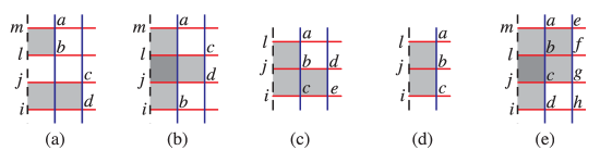
Figure 5. Domains in $\mathcal{H}^{D}$ forcing relations and a differential $\mathcal{A}$. Part (a) forces $\rho_{i,j}$ and $\rho_{l,m}$ to commute. Part (b) forces $\rho_{i,m}$ and $\rho_{j,l}$ to commute. Part (c) forces $\rho_{i,j}\cdot\rho_{j,l}=\rho_{i,l}$. Part (d) forces the algebra to have a differential, and part (e) forces the product $\rho_{i,l}\cdot\rho_{j,m}$ to vanish.

Consider the module $\mathit{CPD}^{-}(\mathcal{H}^{D})$. In Part (a) of Figure 5 is a plausible piece of $\mathcal{H}^{D}$. One sees here several generators; we single out $\{a,c\}$, $\{a,d\}$, $\{b,c\}$ and $\{b,d\}$. Parts of the shaded region contribute to the differential as follows:

$$\partial\{a,c\} =\rho_{l,m}\{b,c\}+\rho_{i,j}\{a,d\}+\cdots$$

$$\partial\{b,c\} =\rho_{i,j}\{b,d\}+\cdots$$

$$\partial\{a,d\} =\rho_{l,m}\{b,d\}+\cdots.$$

(Here, the dots indicate contributions from regions of the diagram other than the shaded one. The philosophy is that cancellation should be local in $\mathcal{H}^{D}$.)

Thus, one has

$$\partial^{2}\{a,c\}=\left(\rho_{l,m}\cdot\rho_{i,j}+\rho_{i,j}\cdot\rho_{l,m}\right)\{b,d\}+\cdots.$$

So, in order to have $\partial^{2}=0$ we should require that $\rho_{i,j}$ and $\rho_{l,m}$ commute.

Similarly, one sees by examining the shaded region in Part (b) of Figure 5 that $\rho_{i,m}$ and $\rho_{j,l}$ should commute.

In Part (c), consider the differentials

$$\partial\{a,d\} =\rho_{i,j}\{a,e\}+\rho_{i,l}\{c,d\}+\cdots$$

$$\partial\{a,e\} =\rho_{j,l}\{b,e\}+\cdots$$

$$\partial\{c,d\} =\{b,e\}+\cdots.$$

Here,

$$\partial^{2}\{a,d\}=\rho_{i,j}\cdot\rho_{j,l}\{b,e\}+\rho_{i,l}\{b,e\}+\cdots.$$

Thus, we should set $\rho_{i,j}\cdot\rho_{j,l}=\rho_{i,l}$—a relation which looks rather reasonable in its own right.

Part (d) is a little trickier. Considering the generators $\{a\}$, $\{b\}$ and $\{c\}$ we have

$$\partial\{a\} =\rho_{j,l}\{b\}+\rho_{i,l}\{c\}+\cdots$$

$$\partial\{b\} =\rho_{i,j}\{c\}+\cdots$$

$$\partial\{c\} =0+\cdots.$$

Thus, it seems we have $\partial^{2}\{a\}=\rho_{j,l}\cdot\rho_{i,j}\{c\}.$ One might try setting $\rho_{j,l}\cdot\rho_{i,j}=0$, but it turns out this is inconsistent with $\mathit{CPA}^{-}$. Instead, we set (in this case)

$$\partial\rho_{i,l}=\rho_{j,l}\cdot\rho_{i,j}.$$

Then it follows that $\partial^{2}\{a\}=0$. Thus, we were forced to introduce a differential on our algebra $\mathcal{A}$.

Note that, in our example, $j\in S(\{a\})$. In general, we define

$$\partial(\rho_{S,i,l})=\sum_{\begin{subarray}{c}j\in S\\ i<j<l\end{subarray}}\rho_{S,j,l}\cdot\rho_{i,j}.$$

This takes care of the example discussed above. The Leibniz rule extends $\partial$ to all of $\mathcal{A}$.

Part (e) is the most complicated. We will consider $\partial^{2}\{b,e\}$. We compute

$$\partial\{b,e\} =\{a,f\}+\rho_{j,l}\{c,e\}+\rho_{i,l}\{d,e\}$$

$$\partial\{a,f\} =\rho_{j,m}\{c,f\}+\rho_{i,m}\{d,f\}+\rho_{j,l}\{a,g\}+\rho_{i,l}\{a,h\}.$$

$$\partial\left(\rho_{j,l}\{c,e\}\right) =\rho_{j,l}\{a,g\}+\rho_{j,m}\{c,f\}+\rho_{j,l}\cdot\rho_{i,j}\{d,e\}$$

$$\partial\left(\rho_{i,l}\{d,e\}\right) =\rho_{j,l}\cdot\rho_{i,j}\{d,e\}+\rho_{i,l}\{a,h\}+\rho_{i,m}\{d,f\}+\rho_{i,l}\cdot\rho_{j,m}\{d,g\}.$$

Most of the terms in $\partial^{2}\{b,e\}$ cancel, but the term $\rho_{i,l}\cdot\rho_{j,m}\{d,g\}$ does not. The offending domain is shaded.

To resolve this difficulty, we impose the relation $\rho_{i,l}\cdot\rho_{j,m}=0$ whenever $i<j<l<m$.

These are essentially all of the cases to check for $\mathit{CPD}^{-}$; we will verify this more carefully in Section 6.

Finally, consider the module $\mathit{CPA}^{-}(\mathcal{H}^{A})$. One must check that the relations we imposed on $\mathcal{A}$ are compatible with the action of $\mathcal{A}$ on $\mathit{CPA}^{-}(\mathcal{H}^{A})$; roughly, this follows by rotating the pictures from Figure 5 by $180$ degrees. We will discuss this more thoroughly in Section 7.

These are the only relations we will need to impose on the algebra $\mathcal{A}$. It turns out—we will see this next—that this algebra has a clean description in terms of strand diagrams.

5. The algebra associated to a slicing

Fix integers $N+1$ and $k$, representing the height and width respectively of a partial planar grid diagram $\mathcal{H}^{A}$. We will define an algebra $\mathcal{A}_{N,k}$. We indicated, in a somewhat roundabout manner, generators and relations for $\mathcal{A}_{N,k}$ in Section 4. We start by giving that definition in a more orderly manner and then move on to a description in terms of strand diagrams.

The algebra $\mathcal{A}_{N,k}$ is free as an $\mathbb{A}$-module. For each $k$-element subset $S$ of $\{0,\dots,N\}$ there is a primitive idempotent $I_{S}$, so that

$$I_{S}\cdot I_{T}=\begin{cases}I_{S}&\text{if $S=T$},\\ 0&\text{otherwise.}\end{cases}$$

The algebra $\mathcal{A}_{N,k}$ is generated as an $\mathbb{A}$-algebra by a set of elements $\rho_{S,i,j}$ (together with the idempotents). Here, $0\leq i<j\leq N$ and $S$ is a $k$-element subset of $\{0,\dots,N\}$ such that $i\in S$ and $j\notin S$. The relations with the idempotents are as follows:

$$I_{T}\cdot\rho_{S,i,j} =\begin{cases}\rho_{S,i,j}&\text{if $S=T$}\\ 0&\text{otherwise}\end{cases}$$

$$\rho_{S,i,j}\cdot I_{T} =\begin{cases}\rho_{S,i,j}&\text{if $T=(S\setminus i)\cup j$}\\ 0&\text{otherwise}.\end{cases}$$

Set $\rho_{i,j}=\sum_{S}\rho_{S,i,j}$, so $\rho_{S,i,j}=I_{S}\rho_{i,j}$. The relations we impose on $\mathcal{A}_{N,k}$ are:

(5.1) $$\rho_{i,j}\cdot\rho_{l,m} =\rho_{l,m}\cdot\rho_{i,j} j<l i<l<m<j$$ for or

(5.2) $$\rho_{i,j}\cdot\rho_{l,m} =0 i<l<j<m$$ for

(5.3) $$\rho_{S,i,j}\cdot\rho_{j,l} =\rho_{S,i,l} j\notin S$$ for .

We also define a differential on $\mathcal{A}_{N,k}$ by setting

$$\partial(\rho_{S,i,j})=\sum_{\begin{subarray}{c}l\in S\\ i<l<j\end{subarray}}\rho_{l,j}\cdot\rho_{i,l}$$

and extending by the Leibniz rule.

Let $\mathcal{I}_{N,k}$ denote the subalgebra of $\mathcal{A}_{N,k}$ generated by the idempotents.

We will check that $\partial^{2}=0$ and that $\partial$ has a consistent extension to all of $\mathcal{A}_{N,k}$, but first we reinterpret this algebra graphically, and introduce a grading.

Let $kI=\coprod_{i=1}^{k}[0,1]$, $\partial_{-}kI=\coprod_{i=1}^{k}\{0\}$ and $\partial_{+}kI=\coprod_{i=1}^{k}\{1\}$. By an upward-veering strand diagram on $k$ strands and $N+1$ positions we mean a class $[\rho]$ of smooth maps

$$\rho\colon(kI,\partial_{-}kI,\partial_{+}kI)\to\left([0,1]\times[0,N],\{0\}\times\{0,\dots,N\},\{1\}\times\{0,\dots,N\}\right)$$

such that $\rho^{\prime}(t)\geq 0$ for all $t\in kI$, and such that the restrictions $\rho|_{\partial_{-}kI}$ and $\rho|_{\partial_{+}kI}$ are injective, modulo homotopy and reordering of the strands. (See Figure 6 for an illustration.) Let $\mathcal{B}(N,k)$ denote the set of upward-veering strand diagrams on $k$ strands and $N+1$ positions.

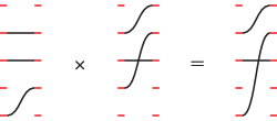
Figure 6. The product on $\mathcal{A}_{4,3}$. Two examples of upward-veering strand diagrams on $3$ strands and $5$ positions are shown left and center, and their product on the right.

Given an element $[\rho]\in\mathcal{B}(N,k)$, let $\operatorname{cr}([\rho])$ denote the minimum number of crossings (double points) of any representative $\rho$ of $[\rho]$.

If $[\rho_{1}],[\rho_{2}]\in\mathcal{B}(N,k)$ are such that $\partial_{+}[\rho_{1}]=\partial_{-}[\rho_{2}]$ then we can concatenate $\rho_{1}$ and $\rho_{2}$ to obtain a new upward-veering strand diagram $\rho_{1}\rho_{2}$. Note that $\operatorname{cr}([\rho_{1}\rho_{2}])\leq\operatorname{cr}([\rho_{1}])+\operatorname{cr}([\rho_{2}])$. Let $\tilde{\mathcal{A}}_{N,k}$ denote the free $\mathbb{A}$-module on $\mathcal{B}(N,k)$, and extend the concatenation operation to a product on $\tilde{\mathcal{A}}_{N,k}$ by setting

$$[\rho_{1}]\cdot[\rho_{2}]=\begin{cases}[\rho_{1}\rho_{2}]&\text{if $\partial_{+}[\rho_{1}]=\partial_{-}[\rho_{2}]$ and $\operatorname{cr}([\rho_{1}\rho_{2}])=\operatorname{cr}([\rho_{1}])+\operatorname{cr}([\rho_{2}])$}\\ 0&\text{otherwise.}\end{cases}$$

This operation is obviously associative. The idempotents of $\tilde{\mathcal{A}}_{N,k}$ are braids consisting of $k$ horizontal strands, and as such are in bijection with the set of $k$-element subsets of $\{1,\dots,N\}$.

We define a differential $\partial$ on $\tilde{\mathcal{A}}_{N,k}$. Given $[\rho]\in\mathcal{B}(N,k)$, with representative $\rho$, let $\operatorname{smooth}(\rho)$ denote the multiset of strand diagrams obtained by smoothing a single crossing in $\rho$. Then define

$$\partial[\rho]=\sum_{\begin{subarray}{c}\rho^{\prime}\in\operatorname{smooth}(\rho)\\ \operatorname{cr}([\rho^{\prime}])=\operatorname{cr}([\rho])-1\end{subarray}}[\rho^{\prime}].$$

See Figure 7.

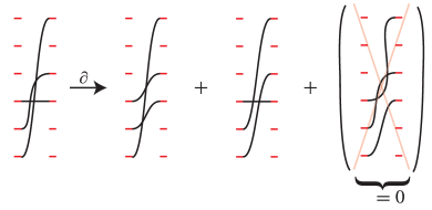
Figure 7. The differential on $\mathcal{A}_{5,3}$. Note that the term on the far right is not included in the differential of the term on the left because of the condition on the number of crossings $\operatorname{cr}$.

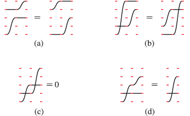
Figure 8. The relations on $\mathcal{A}_{4,2}$. Parts (a) and (b) correspond to relation (5.1). Part (c) corresponds to relation (5.2). Part (d) corresponds to relation (5.3).

Lemma 5.4.

The algebra $\mathcal{A}_{N,k}$ is isomorphic to the algebra $\tilde{\mathcal{A}}_{N,k}$, via an isomorphism identifying the differentials.

Proof.

This is easy to check; see Figure 8 for a convincing illustration that the relations agree. That the differentials agree is similarly straightforward. ∎

Provisionally, we define a grading on $\mathcal{A}_{N,k}$ by setting $\operatorname{gr}([\rho])=\operatorname{cr}([\rho])$.

Proposition 5.5.

The algebra $\mathcal{A}_{N,k}$ is a differential graded algebra. That is:

1. The differential satisfies $\partial^{2}=0$.

2. The differential satisfies the Leibniz rule $\partial(ab)=(\partial a)b+a(\partial b)$.

3. Multiplication has degree $0$.

4. The differential has degree $-1$.

Proof.

All four parts are obvious from the description in terms of strand diagrams. ∎

Remark 5.6.

We have given two different definitions of $\mathcal{A}_{N,k}$. We could give a third, closely related to permutations: the algebra is generated over $\mathbb{A}$ by bijective maps $f\colon S\to T$ between $k$-element subsets of $\{0,\dots,N\}$, such that for all $i\in S$, $f(i)\geq i$. The function $\operatorname{cr}$ is then the number of inversions of the map (i.e., the number of pairs of integers $i<j$ for which $f(i)>f(j)$), and the multiplication is composition if it is defined and preserves $\operatorname{cr}$ and zero otherwise. See [7, Section 3.1.1] for further discussion.

The homological (Maslov) grading we want is not the same as $\operatorname{gr}$. In fact, both the Maslov and Alexander gradings on $\mathcal{A}_{N,k}$ depend not just on $N$ and $k$ but also on which rows contain $X$’s and $O$’s to the left of $Z$.

More precisely, fix $k$-element subsets $L_{X}$ and $L_{O}$ of $\{1/2,\dots,N-1/2\}$, which are the $y$-coordinates of the $X_{i}$’s and $O_{i}$’s contained in $\mathcal{H}^{A}$ (including $X_{k}$). Given an algebra element $a$, viewed as a strand diagram, let $L_{X}(a)$ denote the intersection number of $a$ with the lines $y=\ell$ for $\ell\in L_{X}$. (Equivalently, define $L_{X}(\rho_{i,j})=\#\{\ell\in L_{X}\mid i<\ell<j\}$ and extend to all of $\mathcal{A}_{N,k}$.) Define $L_{O}(a)$ similarly.

For $a\in\mathcal{A}_{N,k}$, define gradings $A$ and $\mu$ by

$$A(a) =L_{X}(a)-L_{O}(a)$$

$$\mu(a) =\operatorname{cr}(a)-2L_{O}(a).$$

It is clear that $A$ is preserved by multiplication and the differential, and that multiplication preserves $\mu$ while the differential drops $\mu$ by $1$.

6. The Type $D$ module

Fix a partial planar grid diagram $\mathcal{H}^{D}$ of height $N+1$ and width $N+1-k$. We will associate to $\mathcal{H}^{D}$ a differential $\mathcal{A}_{N,k}$-module.

We define a left action of the idempotents $\mathcal{I}_{N,k}$ on $\mathbb{A}\langle\mathfrak{S}(\mathcal{H}^{D})\rangle$, the free $\mathbb{A}$-module generated by the generators in $\mathcal{H}^{D}$ (see Section 3). Recall that a generator $\mathbf{x}^{D}\in\mathfrak{S}(\mathcal{H}^{D})$ corresponds to an injection $\sigma_{\mathbf{x}}\colon\{k,\dots,N+1\}\to\{0,\dots,N\}$. So, set

$$I_{S}\mathbf{x}^{D}=\begin{cases}\mathbf{x}^{D}&\text{if $S\cap\mathrm{Im}(\sigma_{\mathbf{x}^{D}})=\emptyset$}\\ 0&\text{otherwise.}\end{cases}$$

As an $\mathcal{A}_{N,k}$-module, let

$$\mathit{CPD}^{-}(\mathcal{H}^{D})=\mathcal{A}_{N,k}\otimes_{\mathcal{I}_{N,k}}\mathbb{A}\langle\mathfrak{S}(\mathcal{H}^{D})\rangle.$$

That is, the module $\mathit{CPD}^{-}(\mathcal{H}^{D})$ is a direct sum of elementary $\mathcal{A}_{N,k}$-modules, one for each generator in $\mathfrak{S}(\mathcal{H}^{D})$.

We next define the differential on $\mathit{CPD}^{-}$. For generators $\mathbf{x}^{D}$ and $\mathbf{y}^{D}$, define $\operatorname{Rect}^{\circ}(\mathbf{x}^{D},\mathbf{y}^{D})$ exactly as in Section 2. Given generators $\mathbf{x}^{D}$, $\mathbf{y}^{D}$ and a segment $\rho_{i,j}$ in $Z$, we define a set $\operatorname{Half}(\rho_{i,j};\mathbf{x},\mathbf{y})$, as follows. Define $\operatorname{Half}(\rho_{i,j};\mathbf{x},\mathbf{y})$ to be empty unless $x_{i}=y_{i}$ for all but one $i$. If $x_{i}=y_{i}$ for $i\neq j$ and the $y$-coordinate of $x_{j}$ is (strictly) greater than the $y$-coordinate of $y_{j}$, then let $\operatorname{Half}(\rho_{i,j};\mathbf{x},\mathbf{y})$ be the singleton set containing the rectangle (or “half-strip”) $H$ with upper right corner $x_{j}$, and lower right corner $y_{j}$, and left edge along the interface $Z$, where it is the segment from $y=i$ to $y=j$. See Figure 9. Call a half strip $H\in\operatorname{Half}(\rho_{i,j};\mathbf{x}^{D},\mathbf{y}^{D})$ empty if the interior of $H$ is disjoint from $\mathbf{x}^{D}$ (or equivalently from $\mathbf{y}^{D}$). Let $\operatorname{Half}^{\circ}(\rho_{i,j};\mathbf{x}^{D},\mathbf{y}^{D})$ denote the set of empty half strips in $\operatorname{Half}(\rho_{i,j};\mathbf{x}^{D},\mathbf{y}^{D})$; this set has at most one element.

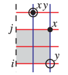
Figure 9. An element (shaded) of $\operatorname{Half}(\rho_{i,j};\mathbf{x},\mathbf{y})$. In fact, the region pictured lies in $\operatorname{Half}^{\circ}(\rho_{i,j};\mathbf{x},\mathbf{y})$. It is also permitted for there to be some $O_{i}$ or $X_{i}$ in the domain (though in the latter case we will not, in fact, count the domain for the theory under discussion).

Now, for $\mathbf{x}^{D}$ a generator, define

$$\partial\mathbf{x}^{D}=\sum_{\mathbf{y}^{D}\in\mathfrak{S}(\mathcal{H}^{D})}\sum_{\begin{subarray}{c}R\in\operatorname{Rect}^{\circ}(\mathbf{x}^{D},\mathbf{y}^{D})\\ \mathbb{X}(R)=0\end{subarray}}U(R)\cdot\mathbf{y}+\sum_{\mathbf{y}^{D}}\sum_{\rho_{i,j}}\sum_{\begin{subarray}{c}H\in\operatorname{Half}^{\circ}(\rho_{i,j};\mathbf{x}^{D},\mathbf{y}^{D})\\ \mathbb{X}(R)=0\end{subarray}}U(H)\cdot\rho_{i,j}\mathbf{y}.$$

We extend the definition via the Leibniz rule to all of $\mathit{CPD}^{-}(\mathcal{H}^{D})$.

Proposition 6.1.

The module $(\mathit{CPD}^{-},\partial)$ is a differential module. That is, $\partial^{2}=0$.

Proof.

Since

$$\partial^{2}(a\mathbf{w}^{D}) =\partial\left((\partial a)\mathbf{w}^{D}+a(\partial\mathbf{w}^{D})\right)$$

$$=\left(\partial^{2}a\right)\mathbf{w}^{D}+2(\partial a)(\partial\mathbf{w}^{D})+a\left(\partial^{2}\mathbf{w}^{D}\right)$$

$$=a\left(\partial^{2}\mathbf{w}^{D}\right),$$

it suffices to show that the coefficient of $\mathbf{y}^{D}$ in $\partial^{2}\mathbf{w}^{D}$ is zero for any $\mathbf{w}^{D},\mathbf{y}^{D}\in\mathfrak{S}(\mathcal{H}^{D})$.

The remainder of the proof is similar to the combinatorial proof in the closed case [9, Proposition 2.8]. Let $a_{\mathbf{w}^{D},\mathbf{x}^{D}}$ denote the coefficient of $\mathbf{x}^{D}$ in $\partial\mathbf{w}^{D}$. Then the coefficient of $\mathbf{y}^{D}$ in $\partial^{2}\mathbf{w}^{D}$ is

(6.2) $$\left(\sum_{\mathbf{x}^{D}}a_{\mathbf{w}^{D},\mathbf{x}^{D}}\cdot a_{\mathbf{x}^{D},\mathbf{y}^{D}}\right)+\partial a_{\mathbf{w}^{D},\mathbf{y}^{D}}.$$

The first term in Formula (6.2) is a sum of terms coming from pairs $(A,B)$ where one of the following cases holds.

1. $A\in\operatorname{Rect}^{\circ}(\mathbf{w}^{D},\mathbf{x}^{D})$ and $B\in\operatorname{Rect}^{\circ}(\mathbf{x}^{D},\mathbf{y}^{D})$ (for some $\mathbf{x}^{D}$). These contributions cancel in pairs exactly as in [9, Proposition 2.8]; see Figure 2.

2. $A\in\operatorname{Rect}^{\circ}(\mathbf{w}^{D},\mathbf{x}^{D})$ and $B\in\operatorname{Half}^{\circ}(\rho_{i,j};\mathbf{x}^{D},\mathbf{y}^{D})$ (for some $\mathbf{x}^{D}$ and $\rho_{i,j}$). There are several cases here, the most interesting of which is illustrated in Figure 5(c). In this case, the relation $\rho_{S,i,j}\cdot\rho_{j,m}=\rho_{S,i,m}$ implies this term cancels with a pair of half strips $(A^{\prime},B^{\prime})$ obtained by cutting the domain horizontally instead of vertically.

3. $A\in\operatorname{Half}^{\circ}(\rho_{i,j};\mathbf{w}^{D},\mathbf{x}^{D})$ and $B\in\operatorname{Half}^{\circ}(\rho_{l,m};\mathbf{x}^{D},\mathbf{y}^{D})$ (for some $\mathbf{x}^{D}$, $\rho_{i,j}$, and $\rho_{l,m}$). Again, there are several cases. The two half-strips may be disjoint (Figure 5(a)), or they may form a sideways “T” (Figure 5(b)); in these two cases, relation (5.1) implies the contributions from taking the two strips in the two different orders cancel. The two half-strips may abut top to bottom, in an “L”-shape (Figure 5(c)); this cancels with one of the cases from Item (2).

   Another possibility is that the upper right corner of $B$ is the lower right corner of $A$, as in Figure 5(d). This configuration contributes a coefficient of $\rho_{j,l}\cdot\rho_{i,j}$ (times some $U$-power). There is also a half-strip, $A\cup B$, which contributes $\rho_{i,l}$ to $\partial\mathbf{w}$; since $\partial\rho_{i,l}=\rho_{j,l}\cdot\rho_{i,j}$ in this case, these terms cancel.

   Finally, the half strips may overlap as in Figure 5(e). But in this case the coefficient contributed is $\rho_{i,l}\cdot\rho_{j,m}$ which is $0$.

Note that all terms in $\partial a_{\mathbf{w}^{D},\mathbf{y}^{D}}$ cancelled against terms in Part (3). This completes the proof. ∎

Finally, we turn to the gradings on $\mathit{CPD}^{-}(\mathcal{H}^{D})$. Fix any planar grid diagram $\mathcal{H}=(\mathbb{R}^{2},\mathbb{X},\mathbb{O})$ such that $\mathcal{H}^{D}=(H^{D},\mathbb{X}^{D},\mathbb{O}^{D})$ can be obtained by cutting $\mathcal{H}$. Then, for a generator $\mathbf{x}^{D}\in\mathfrak{S}(\mathcal{H}^{D})$, there are numbers $\mathcal{I}(\mathbb{X},\mathbf{x}^{D})$ and $\mathcal{I}(\mathbb{O},\mathbf{x}^{D})$, as in Section 2. These numbers obviously do not depend on the choice of $\mathcal{H}$. Further, fix any generator $\mathbf{x}\in\mathfrak{S}(\mathcal{H})$ extending $\mathbf{x}^{D}$. Then we have a number $\mathcal{I}(\mathbf{x},\mathbf{x}^{D})$, which again does not depend on the choice of $\mathcal{H}$ or $\mathbf{x}$. Now, define the gradings of $\mathbf{x}^{D}$ by

$$A(\mathbf{x}^{D}) =\mathcal{I}(\mathbb{X},\mathbf{x}^{D})-\mathcal{I}(\mathbb{O},\mathbf{x}^{D})$$

$$\mu(\mathbf{x}^{D}) =\mathcal{I}(\mathbf{x},\mathbf{x}^{D})-2\mathcal{I}(\mathbb{O},\mathbf{x}^{D}).$$

Extend these definitions to all of $\mathit{CPD}^{-}(\mathcal{H}^{D})$ by setting $A(a\mathbf{x}^{D})=A(a)+A(\mathbf{x}^{D})$ and $\mu(a\mathbf{x}^{D})=\mu(a)+\mu(\mathbf{x}^{D})$ for $a\in\mathcal{A}_{N,k}$.

Proposition 6.3.

The gradings $A$ and $\mu$ make $\mathit{CPD}^{-}(\mathcal{H}^{D})$ into a graded module over $\mathcal{A}_{N,k}$. The differential $\partial$ on $\mathit{CPD}^{-}(\mathcal{H}^{D})$ drops $\mu$ by $1$ while preserving $A$.

(When assigning gradings to the algebra, we let $L_{X}$ denote the set of $i-1/2$ which are not $y$-coordinates of points in $\mathbb{X}^{D}$, and similarly for $L_{O}$.)

Proof.

The first statement is trivial. To verify that the differential drops $\mu$ by $1$, write $\mathbf{x}=(\mathbf{x}^{A},\mathbf{x}^{D})$. Suppose that $\left(\prod_{\ell}U_{\ell}^{n_{\ell}}\right)\rho_{i,j}\cdot\mathbf{y}^{D}$ occurs in $\partial\mathbf{x}^{D}$. Then

$$\mathcal{I}(\mathbf{x},\mathbf{x}^{D})-\mathcal{I}(\mathbf{y},\mathbf{y}^{D})=1+\#\{(r,s)\in\mathbf{x}^{A}\mid i<s<j\}.$$

This is exactly $1+\operatorname{cr}(\rho_{S,i,j})$, where $S=\{0,\dots,N\}\setminus\mathrm{Im}(\sigma_{\mathbf{x}^{D}})$. Also,

$$\mathcal{I}(\mathbb{O},\mathbf{x}^{D})-\mathcal{I}(\mathbb{O},\mathbf{y}^{D})=\left(\sum_{\ell}n_{\ell}\right)+L_{O}(\rho_{i,j}).$$

This implies that the differential decreases $\mu$ by $1$, as desired. That the differential preserves $A$ is similar but easier. ∎

7. The Type $A$ module

The module $\mathit{CPA}^{-}$ is much smaller than $\mathit{CPD}^{-}$. Fix a partial planar grid diagram $\mathcal{H}^{A}$ with width $k$ and height $N+1$. The module $\mathit{CPA}^{-}(\mathcal{H}^{A})$ is freely generated over $\mathbb{A}$ by $\mathfrak{S}(\mathcal{H}^{A})$. There is a differential $\partial$ on $\mathit{CPA}^{-}(\mathcal{H}^{A})$ defined by

$$\partial\mathbf{x}^{A}=\sum_{\mathbf{y}^{A}\in\mathfrak{S}(\mathcal{H}^{A})}\sum_{\begin{subarray}{c}R\in\operatorname{Rect}^{\circ}(\mathbf{x}^{A},\mathbf{y}^{A})\\ \mathbb{X}(R)=0\end{subarray}}U(R)\cdot\mathbf{y}^{A}.$$

It remains to define an action of $\mathcal{A}_{N,k}$ on $\mathit{CPA}^{-}(\mathcal{H}^{A})$.

Given a generator $\mathbf{x}^{A}\in\mathfrak{S}(\mathcal{H}^{A})$, let $\sigma_{\mathbf{x}^{A}}$ denote the corresponding map $\{0,\dots,k-1\}\allowbreak\to\{0,\dots,N\}$. We define an action of the idempotents $\mathcal{I}_{N,k}$ by

$$\mathbf{x}^{A}I_{S}=\begin{cases}\mathbf{x}^{A}&\text{if $S=\mathrm{Im}(\sigma_{\mathbf{x}^{A}})$}\\ 0&\text{otherwise.}\end{cases}$$

This is, in some sense, exactly the opposite of the action of the idempotents on $\mathit{CPD}^{-}$.

Given generators $\mathbf{x}^{A}$ and $\mathbf{y}^{A}$ in $\mathfrak{S}(\mathcal{H}^{A})$ and a generator $\rho_{i,j}$ of $\mathcal{A}_{N,k}$ (which we view as a chord in $Z$ from $y=i$ to $y=j$) define $\operatorname{Half}(\mathbf{x},\mathbf{y};\rho_{i,j})$ to be empty unless $x_{k}=y_{k}$ for all but one $k$, and in this case let it be the singleton set containing the rectangle (or “half-strip”) $H$ with lower left corner $x_{k}$ and upper left corner $y_{k}$, and right edge $\rho_{i,j}$ if such a rectangle exists, and empty otherwise. See Figure 10. Call a half strip $H\in\operatorname{Half}(\mathbf{x}^{A},\mathbf{y}^{A};\rho_{i,j})$ empty if the interior of $H$ is disjoint from $\mathbf{x}^{A}$. Let $\operatorname{Half}^{\circ}(\mathbf{x}^{A},\mathbf{y}^{A};\rho_{i,j})$ denote the set of empty half strips in $\operatorname{Half}(\mathbf{x}^{A},\mathbf{y}^{A};\rho_{i,j})$.

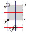
Figure 10. An element of $\operatorname{Half}(\mathbf{x},\mathbf{y};\rho_{i,j})$. The definition is essentially the same as the definition for $\mathit{CPD}^{-}$, only rotated by $180$ degrees.

We define an action by the generators $\rho_{i,j}$ of $\mathcal{A}_{N,k}$ by

$$\mathbf{x}^{A}\rho_{i,j}=\sum_{\begin{subarray}{c}\mathbf{y}^{A}\in\mathfrak{S}(\Sigma)\\ H\in\operatorname{Half}^{\circ}(\mathbf{x}^{A},\mathbf{y}^{A};\rho_{i,j})\\ \mathbb{X}(H)=0\end{subarray}}U(H)\cdot\mathbf{y}^{A}.$$

(The sum contains at most one term.)

Proposition 7.1.

The module $\mathit{CPA}^{-}(\mathcal{H}^{A})$ is a differential $\mathcal{A}_{N,k}$-module. That is:

1. The action of the $\rho_{i,j}$ defined above respects the relations in $\mathcal{A}_{N,k}$.

2. The action satisfies the Leibniz rule.

3. The differential $\partial$ satisfies $\partial^{2}=0$.

Proof.

(The reader may wish to compare this with the proof of Proposition 6.1: the pictures are almost the same, but their interpretations are different.)

That the $\mathcal{A}_{N,k}$-action respects the three relations (5.1), (5.2) and (5.3) follow from the cases illustrated in Figure 11. In parts (a) and (b), we have

$$\left(\{a,c\}\rho_{i,j}\right)\rho_{l,m}=\left(\{a,c\}\rho_{l,m}\right)\rho_{i,j}=\{b,d\}.$$

so relation (5.1) is respected. (We suppress the $U$-powers, but since these depend only on the domains they, too, agree.)

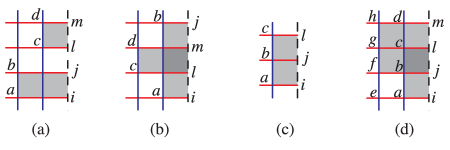
Figure 11. The $\mathcal{A}_{N,k}$-action on $\mathit{CPA}^{-}$ respects the relations on the algebra. Parts (a) and (b) correspond to relation (5.1). Part (c) corresponds to relation (5.2). Part (d) corresponds to relation (5.3).

In part (c) of Figure 11,

$$(\{a\}\rho_{i,j})\rho_{j,l}=\{b\}\rho_{j,l}=\{c\}=\{a\}\rho_{i,l},$$

so relation (5.2) is respected.

In part (d) of Figure 11 we have

$$\left(\{a,f\}\rho_{i,l}\right)\rho_{j,m}=\{c,f\}\rho_{j,m}=0$$

since the corresponding half-strip is not empty. So, relation (5.3) is respected. (This is only one of the two pictures we need to check in this case, but the other is similar.)

This proves Part (1).

Part (2) follows from Figure 12. More precisely, it suffices to show that for any $i,j$,

$$\partial\left(\mathbf{x}^{A}\rho_{i,j}\right)=\left(\partial\mathbf{x}^{A}\right)\rho_{i,j}+\mathbf{x}^{A}\left(\partial\rho_{i,j}\right).$$

Both $\partial\left(\mathbf{x}^{A}\rho_{i,j}\right)$ and $\left(\partial\mathbf{x}^{A}\right)\rho_{i,j}$ correspond to a domain which is a union of a rectangle and a half-strip. The most interesting case is when these abut to form an “L”-shape, as in Figure 12. There, for $\mathbf{x}^{A}=\{b,d\}$ we have

$$\partial\{b,d\} =\{a,e\}$$

$$\{a,e\}\rho_{i,l} =\{c,e\}$$

$$\{b,d\}\rho_{j,l}\rho_{i,j} =\{c,e\}$$

$$\{b,d\}\rho_{i,l} =0,$$

so

$$\partial\left(\{b,d\}\rho_{i,l}\right)=0=\left(\partial\{b,d\}\right)\rho_{i,l}+\{b,d\}\left(\partial\rho_{i,l}\right).$$

(The other interesting but similar case is obtained by flipping Figure 12 vertically.) This proves Part 2.

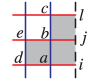
Figure 12. The Leibniz rule for $\mathit{CPA}^{-}$. The domain shown can be decomposed in two ways: as a rectangle followed by a half-strip, or as two half strips. These correspond to $\left(\partial\{b,d\}\right)\rho_{i,l}$ and $\{b,d\}\left(\partial\rho_{i,l}\right)$ respectively.

Part (3) follows from the same argument as in the closed case [9, Proposition 2.8]; see also Figure 2. ∎

Finally, we turn to the gradings on $\mathit{CPA}^{-}(\mathcal{H}^{A})$. Define

$$A(\mathbf{x}^{A}) =\mathcal{I}(\mathbb{X}^{A},\mathbf{x}^{A})-\mathcal{I}(\mathbb{O}^{A},\mathbf{x}^{A})$$

$$\mu(\mathbf{x}^{D}) =\mathcal{I}(\mathbf{x}^{A},\mathbf{x}^{A})-2\mathcal{I}(\mathbb{O}^{A},\mathbf{x}^{A}).$$

Proposition 7.2.

These gradings make $\mathit{CPA}^{-}(\mathcal{H}^{A})$ into a graded $\mathcal{A}_{N,k}$-module. The differential on $\mathit{CPA}^{-}(\mathcal{H}^{A})$ preserves the Alexander grading $A$ and drops the Maslov grading $\mu$ by $1$.

(When assigning gradings to the algebra, we let $L_{X}$ denote the set of $i-1/2$ which are $y$-coordinates of points in $\mathbb{X}^{A}$, and similarly for $L_{O}$.)

Proof.

We check that multiplication preserves the $A$ grading. Suppose $\mathbf{x}^{A}\rho_{i,j}=\left(\prod_{\ell}U_{\ell}^{n_{\ell}}\right)\mathbf{y}^{A}$. Then

$$\mathcal{I}(\mathbb{X}^{A},\mathbf{x}^{A}) =\mathcal{I}(\mathbb{X}^{A},\mathbf{y}^{A})-L_{X}(\rho_{i,j})$$

$$\mathcal{I}(\mathbb{O}^{A},\mathbf{x}^{A}) =\mathcal{I}(\mathbb{O}^{A},\mathbf{y}^{A})-L_{O}(\rho_{i,j})+\sum_{\ell}n_{\ell}.$$

The result follows.

That multiplication preserves $\mu$ is similar; see also the proof of Proposition 6.3 That the differential preserves $A$ and drops $\mu$ by $1$ is straightforward. ∎

Remark 7.3.

The definition of $\mathit{CPA}^{-}$ is somewhat different in spirit from the definition of $\widehat{\mathit{CFA}}$ for bordered three-manifolds in [7, Section 7]: there the product $\mathbf{x}^{A}a$ is defined directly for any algebra element $a$. In our setting, we could do this by counting more complicated domains than rectangles.

8. The pairing theorem

Theorem 2.

Let $\mathcal{H}$ be a planar grid diagram, decomposed as $\mathcal{H}^{A}\cup_{Z}\mathcal{H}^{D}$, where $\mathcal{H}^{A}$ (respectively $\mathcal{H}^{D}$) is a partial planar grid diagram with width $k$ (respectively $N+1-k$) and height $N+1$. Then

$$\mathit{CP}^{-}(\mathcal{H})\cong\mathit{CPA}^{-}(\mathcal{H}^{A})\otimes_{\mathcal{A}_{N,k}}\mathit{CPD}^{-}(\mathcal{H}^{D}),$$

as $(\mathbb{Z}\oplus\mathbb{Z})$-graded chain complexes over $\mathbb{A}$.

Proof.

There is an obvious identification between the generators of $\mathit{CP}^{-}(\mathcal{H})$ and the generators of $\mathit{CPA}^{-}(\mathcal{H}^{A})\otimes_{\mathcal{A}_{N,k}}\mathit{CPD}^{-}(\mathcal{H}^{D})$. It follows from their definitions that this identification respects the $A$ and $\mu$ gradings.

The rest of the proof is essentially trivial, so we write it with formulas to make it seem complicated. Given a generator $\mathbf{x}$ of $\mathit{CP}^{-}(\mathcal{H})$, we split $\partial\mathbf{x}$ into three pieces, according to whether the domain rectangle is entirely to the left of the dividing line $\{x=k-1/4\}$, crosses the dividing line, or is entirely to the right of the dividing line:

$$\partial\mathbf{x}=\partial_{L}\mathbf{x}+\partial_{M}\mathbf{x}+\partial_{R}\mathbf{x}.$$

Then if $\mathbf{x}$ is identified with $\mathbf{x}^{A}\otimes\mathbf{x}^{D}$, we have

$$\partial(\mathbf{x}^{A}\otimes\mathbf{x}^{D}) =(\partial\mathbf{x}^{A})\otimes\mathbf{x}^{D}+\mathbf{x}^{A}\otimes(\partial\mathbf{x}^{D})$$

$$=\partial_{L}\mathbf{x}+\partial_{R}\mathbf{x}+\sum_{\mathbf{y}^{D}\in\mathfrak{S}(\mathcal{H}^{D})}\sum_{\begin{subarray}{c}H\in\operatorname{Half}^{\circ}(\rho_{i,j};\mathbf{x}^{D},\mathbf{y}^{D})\\ \mathbb{X}(H)=0\end{subarray}}U(H)(\mathbf{x}^{A}\otimes\rho_{i,j}\mathbf{y}^{D})$$

$$=\partial_{L}\mathbf{x}+\partial_{R}\mathbf{x}+\sum_{\mathbf{y}^{D}\in\mathfrak{S}(\mathcal{H}^{D})}\sum_{\begin{subarray}{c}H\in\operatorname{Half}^{\circ}(\rho_{i,j};\mathbf{x}^{D},\mathbf{y}^{D})\\ \mathbb{X}(H)=0\end{subarray}}U(H)(\mathbf{x}^{A}\rho_{i,j}\otimes\mathbf{y}^{D})$$

$$=\partial_{L}\mathbf{x}+\partial_{R}\mathbf{x}$$

$$\qquad+\sum_{\begin{subarray}{c}\mathbf{y}^{D}\in\mathfrak{S}(\mathcal{H}^{D})\\ \mathbf{y}^{A}\in\mathfrak{S}(\mathcal{H}^{A})\\ \rho_{i,j}\end{subarray}}\,\sum_{\begin{subarray}{c}H\in\operatorname{Half}^{\circ}(\rho_{i,j};\mathbf{x}^{D},\mathbf{y}^{D})\\ \mathbb{X}(H)=0\end{subarray}}\,\sum_{\begin{subarray}{c}H^{\prime}\in\operatorname{Half}^{\circ}(\mathbf{x}^{A},\mathbf{y}^{A};\rho_{i,j})\\ \mathbb{X}(H^{\prime})=0\end{subarray}}U(H^{\prime}\cup H)(\mathbf{y}^{A}\otimes\mathbf{y}^{D})$$

$$=\partial_{L}\mathbf{x}+\partial_{R}\mathbf{x}+\partial_{M}\mathbf{x}$$

$$=\partial\mathbf{x},$$

as desired. ∎

Remark 8.1.

More useful is the fact that $\mathit{CP}^{-}(\mathcal{H})$ is quasi-isomorphic to the derived tensor product $\mathit{CPA}^{-}(\mathcal{H}^{A})\mathop{\widetilde{\otimes}}\nolimits_{\mathcal{A}_{N,k}}\mathit{CPD}^{-}(\mathcal{H}^{D})$. For instance, this allows one to simplify the complexes $\mathit{CPA}^{-}$ and $\mathit{CPD}^{-}$ more dramatically before taking the tensor product. In fact, the $\mathcal{A}_{N,k}$-module $\mathit{CPD}^{-}(\mathcal{H}^{D})$ is projective (hence flat), as one can see by imitating an argument from Bernstein and Lunts [1, Proposition 10.12.2.6]. It follows that the derived tensor product agrees with the ordinary one.

9. Bimodules

At this point we have encountered left and right modules over $\mathcal{A}_{N,k}$. We will now see that bimodules also have several important roles to play. (The material in this section is analogous to material in [6].)

9.1. Freezing

We have studied how to take a planar grid diagram and make a single vertical cut. In the spirit of factoring a braid into generators, however, we might want to make several different vertical cuts. In this section we will see that the correct objects to assign to slices in the middle are $(\mathcal{A}_{N,k}$,$\mathcal{A}_{N,l})$-bimodules.

That is, consider the result of slicing a planar grid diagram $\mathcal{H}$ along the lines $Z_{1}=\{x=k-1/4\}$ and $Z_{2}=\{x=l-1/4\}$ (with $l>k$). The result is two partial planar grid diagrams $\mathcal{H}^{A}=\mathcal{H}\cap\{x<k-1/4\}$ and $\mathcal{H}^{D}=\mathcal{H}\cap\{x>l-1/4\}$, and a middle partial planar grid diagram $\mathcal{H}^{DA}=\mathcal{H}\cap\{k-1/4<x<l-1/4\}$. We will associate an $(\mathcal{A}_{N,k},\mathcal{A}_{N,l})$-bimodule $\mathit{CPDA}^{-}(\mathcal{H}^{DA})$ to $\mathcal{H}^{DA}$.

A generator for $\mathcal{H}^{DA}$ is an $(l-k)$-tuple of points $\mathbf{x}=\{x_{i}\}_{i=k}^{l-1}$; a generator $\mathbf{x}$ corresponds to an injection $\sigma_{\mathbf{x}}\colon\{k,\dots,l-1\}\to\{1,\dots,N\}$. (For consistency with earlier notation, we should really write $\mathbf{x}$ as $\mathbf{x}^{DA}$, but the notation becomes too cumbersome.) Let $\mathfrak{S}(\mathcal{H}^{DA})$ denote the set of generators for $\mathcal{H}^{DA}$. Call a generator $\mathbf{x}$ compatible with an idempotent $I_{S}\in\mathcal{A}_{N,k}$ if $\mathrm{Im}(\sigma_{\mathbf{x}})\cap S=\emptyset$. As a left module, $\mathit{CPDA}^{-}(\mathcal{H}^{DA})$ is a direct sum of elementary modules,

$$\mathit{CPDA}^{-}(\mathcal{H}^{DA})=\bigoplus_{\begin{subarray}{c}\mathbf{x}\in\mathfrak{S}(\mathcal{H}^{DA})\\ S\text{ compatible with }\mathbf{x}\end{subarray}}\mathcal{A}_{N,k}I_{S}.$$

We will write the generator of the summand $\mathcal{A}_{N,k}I_{S}$ coming from $\mathbf{x}$ as $I_{S}\mathbf{x}.$ Note that, unlike for $\mathit{CPD}^{-}$ or $\mathit{CPA}^{-}$, the generator $\mathbf{x}$ does not determine the idempotent $S$.

We next define a differential on $\mathit{CPDA}^{-}(\mathcal{H}^{DA})$. Given generators $\mathbf{x},\mathbf{y}\in\mathfrak{S}(\mathcal{H}^{DA})$ such that $x_{n}=y_{n}$ for $n\neq m$ (for some $m$), and $i<j\in\{0,\dots,N\}$, define $\operatorname{Half}(\rho_{i,j};\mathbf{x},\mathbf{y})$ to be the set of rectangles with upper right corner at $x_{m}$, lower right corner at $y_{m}$ and left edge the segment $\rho_{i,j}$ in $Z_{1}$ from $(k-1/4,i)$ to $(k-1/4,j)$. Define $\operatorname{Half}^{\circ}(\rho_{i,j};\mathbf{x},\mathbf{y})$ to be the subset of $\operatorname{Half}(\rho_{i,j};\mathbf{x},\mathbf{y})$ consisting of empty half-strips, i.e., half strips not containing any element of $\mathbf{x}$ in their interiors. Then set

$$\partial(I_{S}\mathbf{x})=\sum_{\mathbf{y}\in\mathfrak{S}(\mathcal{H}^{DA})}\,\sum_{\begin{subarray}{c}R\in\operatorname{Rect}^{\circ}(\mathbf{x},\mathbf{y})\\ \mathbb{X}(R)=0\end{subarray}}U(R)\cdot I_{S}\mathbf{y}+\sum_{\begin{subarray}{c}\mathbf{y}\in\mathfrak{S}(\mathcal{H}^{DA})\\ i<j\in\{0,\dots,N\}\end{subarray}}\sum_{\begin{subarray}{c}H\in\operatorname{Half}^{\circ}(\rho_{i,j};\mathbf{x},\mathbf{y})\\ \mathbb{X}(H)=0\end{subarray}}U(H)\cdot I_{S}\rho_{i,j}\mathbf{y}.$$

Here, the notation $I_{S}\rho_{i,j}\mathbf{y}$, though suggestive, should be explained. If $i\in S$ and $j\notin S$ then $I_{S}\rho_{i,j}\mathbf{y}$ denotes $\rho_{i,j}I_{T}$, where $T=(S\setminus i)\cup j$, if $T$ is compatible with $\mathbf{y}$. Otherwise (i.e., if $i\notin S$, $j\in S$, or $T$ is not compatible with $\mathbf{y}$) we declare $I_{S}\rho_{i,j}\mathbf{y}$ to be $0$.

Finally, we define the right module structure on $\mathit{CPDA}^{-}(\mathcal{H}^{DA})$. Given a primitive idempotent $I_{T}\in\mathcal{I}_{N,l}$, define

$$(I_{S}\mathbf{x})I_{T}=\begin{cases}I_{S}\mathbf{x}&\text{if $\left(S\cup\mathrm{Im}(\sigma_{\mathbf{x}})\right)\cap T=\emptyset$}\\ 0&\text{otherwise}.\end{cases}$$

Given generators $\mathbf{x},\mathbf{y}\in\mathfrak{S}(\mathcal{H}^{DA})$ such that $x_{\ell}=y_{\ell}$ for $\ell\neq m$ (for some $m$), and $i<j\in\{0,\dots,N\}$, define $\operatorname{Half}(\mathbf{x},\mathbf{y};\rho_{i,j})$ to be the set of rectangles with lower left corner at $x_{m}$, upper left corner at $y_{m}$ and right edge the segment $\rho_{i,j}$ in $Z_{2}$ from $(l-1/4,i)$ to $(l-1/4,j)$. Define $\operatorname{Half}^{\circ}(\mathbf{x},\mathbf{y};\rho_{i,j})$ to be the subset of $\operatorname{Half}(\mathbf{x},\mathbf{y};\rho_{i,j})$ consisting of empty half-strips, i.e., half strips not containing any element of $\mathbf{x}$ in their interiors.

Given a chord $\rho_{i,j}$ in $Z_{2}$ from $(l-1/4,i)$ to $(l-1/4,j)$, define $\operatorname{Strip}(\rho_{i,j})$ to be the horizontal strip with right edge $\rho_{i,j}\subset Z_{2}$ and left edge $\rho_{i,j}\subset Z_{1}$. Given $\rho_{i,j}$ and a generator $\mathbf{x}\in\mathfrak{S}(\mathcal{H}^{DA})$, define $\operatorname{Strip}^{\circ}(\mathbf{x};\rho_{i,j})$ to be the empty set if $\operatorname{Strip}(\rho_{i,j})$ contains a point in $\mathbf{x}$ (even along its boundary) and the singleton set $\operatorname{Strip}(\rho_{i,j})$ if $\operatorname{Strip}(\rho_{i,j})$ does not contain a point in $\mathbf{x}$.

At last, define

$$(I_{S}\mathbf{x})\rho_{i,j}=\sum_{\begin{subarray}{c}E\in\operatorname{Strip}^{\circ}(\mathbf{x},\rho_{i,j})\\ \mathbb{X}(E)=0\end{subarray}}U(E)\cdot I_{S}\rho_{i,j}\mathbf{x}+\sum_{\mathbf{y}\in\mathfrak{S}(\mathcal{H}^{DA})}\sum_{\begin{subarray}{c}H\in\operatorname{Half}^{\circ}(\mathbf{x},\mathbf{y};\rho_{i,j})\\ \mathbb{X}(H)=0\end{subarray}}U(H)\cdot I_{S}\mathbf{y}.$$

These definitions are, in fact, compatible:

Proposition 9.1.

The module $\mathit{CPDA}^{-}(\mathcal{H}^{DA})$ is a differential $(\mathcal{A}_{N,k},\mathcal{A}_{N,l})$-bimodule.

We leave the proof to the interested reader.

As on $\mathit{CPD}^{-}$, the grading of a generator $I_{S}\mathbf{x}$ of $\mathit{CPDA}^{-}(\mathcal{H}^{DA})$ is given by

$$A(I_{S}\mathbf{x}) =\mathcal{I}(\mathbb{X},\mathbf{x})-\mathcal{I}(\mathbb{O},\mathbf{x})$$

$$\mu(I_{S}\mathbf{x}) =\mathcal{I}(\bar{\mathbf{x}},\mathbf{x})-2\mathcal{I}(\mathbb{O},\mathbf{x}),$$

where $\mathcal{H}=(\mathbb{R}^{2},\mathbb{X},\mathbb{O})$ is any planar diagram completing $\mathcal{H}^{DA}$, and $\bar{\mathbf{x}}$ is a generator in $\mathfrak{S}(\mathcal{H})$ completing $\mathbf{x}$ and compatible with the idempotent $I_{S}$ in the obvious sense.

Finally, the module $\mathit{CPDA}^{-}(\mathcal{H}^{DA})$ satisfies a pairing theorem:

Proposition 9.2.

With notation as above,

$$\mathit{CPA}^{-}(\mathcal{H}^{A}\cup_{Z_{1}}\mathcal{H}^{DA}) =\mathit{CPA}^{-}(\mathcal{H}^{A})\otimes_{\mathcal{A}_{N,k}}\mathit{CPDA}^{-}(\mathcal{H}^{DA})$$

$$\mathit{CPD}^{-}(\mathcal{H}^{DA}\cup_{Z_{2}}\mathcal{H}^{D}) =\mathit{CPDA}^{-}(\mathcal{H}^{DA})\otimes_{\mathcal{A}_{N,l}}\mathit{CPD}^{-}(\mathcal{H}^{D})$$

$$\mathit{CP}^{-}(\mathcal{H}) =\mathit{CPA}^{-}(\mathcal{H}^{A})\otimes_{\mathcal{A}_{N,k}}\mathit{CPDA}^{-}(\mathcal{H}^{DA})\otimes_{\mathcal{A}_{N,l}}\mathit{CPD}^{-}(\mathcal{H}^{D}).$$

The proof is obvious. The analogous result for cutting along more than two vertical lines is also true.

Remark 9.3.

The notation $\mathit{CPDA}^{-}$ denotes that the module is “Type $D$” from the left and “Type $A$” from the right.

9.2. Type $A$ to Type $D$

The reader might wonder about the relation between $\mathit{CPA}^{-}$ and $\mathit{CPD}^{-}$. One might expect that they are, in some appropriate sense, dual to each other. In the case of bordered Heegaard Floer homology this is true. In this section, we hint at that story by reconstructing $\mathit{CPD}^{-}$ from $\mathit{CPA}^{-}$. In Section 9.3 we will discuss going the other direction. We will suppress both the gradings and the $U$-variables: our treatment of both has been too naïve to extend properly to the present discussion.

Let $k^{\prime}=N+1-k$. We construct a $(\mathcal{A}_{N,k},\mathcal{A}_{N,k^{\prime}})$-bimodule $\mathit{CPDD}^{-}_{N,k}$ so that $\mathit{CPD}^{-}(\mathcal{H}^{D})=\mathit{CPA}^{-}(\mathcal{H}^{D})\otimes_{\mathcal{A}_{N,k}}\mathit{CPDD}^{-}_{N,k}$. Actually, unlike a traditional bimodule with a left action and a right action, we will construct the $\mathcal{A}_{N,k}$- and $\mathcal{A}_{N,k^{\prime}}$-actions as a pair of commuting left actions, so the module $\mathit{CPA}^{-}(\mathcal{H}^{D})\otimes_{\mathcal{A}_{N,k}}\mathit{CPDD}^{-}_{N,k}$ comes equipped with a left action rather than a right action.

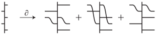
Figure 13. A graphical representation of $\mathit{CPDD}^{-}_{N,k}$. The case shown is $N=4$, $k=2$. The element $I_{S}$, for $S=\{1,3\}$, is shown on the left. On the right is the differential of $I_{S}\otimes 1$. This graphical representation treats $\mathit{CPDD}^{-}_{N,k}$ as a traditional (left,right) bimodule, rather than a (left,left) bimodule; this is the reason that the strands on the right are downward-veering.

The module $\mathit{CPDD}^{-}_{N,k}$ is easy to describe. Note that there is an obvious isomorphism $\mathcal{I}_{N,k}\to\mathcal{I}_{N,k^{\prime}}$, taking $I_{S}$ to $I_{\{0,\dots,N\}\setminus S}$. This makes $\mathcal{A}_{N,k^{\prime}}$ into a right $\mathcal{I}_{N,k}$-module. The module $\mathit{CPDD}^{-}_{N,k}$ is just

$$\mathcal{A}_{N,k^{\prime}}\otimes_{\mathcal{I}_{N,k}}\mathcal{A}_{N,k^{\prime}}$$

where the tensor product identifies the right actions of $\mathcal{I}_{N,k}$ on $\mathcal{A}_{N,k^{\prime}}$ and $\mathcal{A}_{N,k^{\prime}}$. This module, then, is equipped with two left actions. The differential on $\mathit{CPDD}^{-}_{N,k}$ is not the one inherited from the tensor product. Rather, for $S$ a $k$-element subset of $\{0,\dots,N\}$ we define

$$\partial(I_{S}\otimes 1)=\sum_{\begin{subarray}{c}i\in S\\ j>i\\ j\notin S\end{subarray}}\rho_{i,j}^{k}\rho_{i,j}^{k^{\prime}}(I_{T}\otimes 1)$$

where $\rho_{i,j}^{k}$ denotes the element $\rho_{i,j}$ of $\mathcal{A}_{N,k}$, $\rho_{i,j}^{k^{\prime}}$ denotes the element $\rho_{i,j}$ of $\mathcal{A}_{N,k^{\prime}}$, and $T=(S\setminus i)\cup j$. We extend the differential to all of $\mathit{CPDD}^{-}_{N,k}$ by the Leibniz rule. An example is illustrated in Figure 13.

Lemma 9.4.

The module $\mathit{CPDD}^{-}_{N,k}$ is a differential $(\mathcal{A}_{N,k},\mathcal{A}_{N,k^{\prime}})$-bimodule.

Proof.

This is immediate from the definitions. ∎

One can view the module $\mathit{CPDD}^{-}_{N,k}$ as the (Type $D$, Type $D$) module associated to a middle partial planar grid diagram with zero $\beta$-lines (i.e., in the notation of Section 9.1, $k=l$). The generator corresponds to the empty set in ${\boldsymbol{\alpha}}\cap{\boldsymbol{\beta}}$. The differential comes from the strips $\operatorname{Strip}(\rho_{i,j})$ (as in Section 9.1).

As promised, we have the following pairing theorem:

Proposition 9.5.

Fix a partial Heegaard diagram $\mathcal{H}^{D}$. Then

$$\mathit{CPD}^{-}(\mathcal{H}^{D})=\mathit{CPA}^{-}(\mathcal{H}^{D})\otimes_{\mathcal{A}_{N,k}}\mathit{CPDD}^{-}_{N,k}.$$

Proof.

The tensor product $\mathit{CPA}^{-}(\mathcal{H}^{D})\otimes_{\mathcal{A}_{N,k}}\mathit{CPDD}^{-}_{N,k}$ is a direct sum of elementary modules $\mathbf{x}^{A}\otimes\mathcal{A}_{N,k^{\prime}}I_{S}$, one for each generator $\mathbf{x}^{A}$ of $\mathit{CPA}^{-}(\mathcal{H}^{D})$, where $S=\{0,\dots,N\}\setminus\mathrm{Im}(\sigma_{\mathbf{x}^{A}})$. The part of the differential on the tensor product coming from the differential on $\mathit{CPA}^{-}(\mathcal{H}^{D})$ counts empty rectangles. The part of the differential coming from the differential on $\mathit{CPDD}^{-}_{N,k}$ counts empty half strips, exactly as on $\mathit{CPD}^{-}(\mathcal{H}^{D})$. ∎

9.3. Remarks on Type $D$ to Type $A$

Turning the module $\mathit{CPD}^{-}$ into $\mathit{CPA}^{-}$ is more subtle than turning $\mathit{CPA}^{-}$ into $\mathit{CPD}^{-}$. It is clearly not possible to find a module $\mathit{CPAA}^{-}_{N,k}$ so that $\mathit{CPA}^{-}$ is exactly equal to $\mathit{CPAA}^{-}_{N,k}\otimes_{\mathcal{A}_{N,k^{\prime}}}\mathit{CPD}^{-}$: the ranks of these modules over $\mathbb{A}$ prevent this.

There are two approaches one might take. One approach is to use properties of $\mathit{CPDD}^{-}_{N,k}$ to prove that it induces an equivalence of categories $\mathcal{D}^{b}(\mathcal{A}_{N,k}-\mathsf{Mod})\to\mathcal{D}^{b}(\mathcal{A}_{N,k^{\prime}}-\mathsf{Mod})$, and then construct a bimodule giving the inverse equivalence of categories.

Another approach is to define $\mathit{CPAA}^{-}_{N,k}$ as an $\mathcal{A}_{\infty}$-bimodule. Using the appropriate model for the $\mathcal{A}_{\infty}$-tensor product (see, e.g., [7, Section 2]), it is then possible for $\mathit{CPA}^{-}$ to be exactly $\mathit{CPAA}^{-}_{N,k}\otimes_{\mathcal{A}_{N,k^{\prime}}}\mathit{CPD}^{-}$. The generators and first few $\mathcal{A}_{\infty}$-operations for this $\mathit{CPAA}^{-}_{N,k}$ are easy to guess. As an $\mathbb{A}$-module, $\mathit{CPAA}^{-}_{N,k}$ would be just $\mathcal{I}_{N,k}\cong\mathcal{I}_{N,k^{\prime}}$. The first few $\mathcal{A}_{\infty}$-relations would be

$$m_{1}(I_{S}) =0$$

$$m_{2}(a,I_{S}) =0$$

$$m_{2}(I_{S},a) =0$$

$$m_{3}(\rho_{i,j},I_{S},\rho_{i,j}) =\begin{cases}I_{T}&\text{ if $i\in S$, $j\notin S$, and where $T=(S\setminus i)\cup j$}\\ 0&\text{otherwise.}\end{cases}$$

(Even though $\mathit{CPAA}^{-}_{N,k}$ should really have two right actions, for clarity we have written it with one right and one left action.)

Unfortunately, higher $\mathcal{A}_{\infty}$-relations are harder to guess and, at least in the case of bordered Heegaard Floer homology, depend on some choices. Fortunately, in the case of bordered Heegaard Floer homology, these modules are induced by counts of holomorphic curves, so we need not build them by hand; see [7]. (In particular, it turns out that the choices are induced by a choice of almost complex structure.) The challenge in defining $\mathit{CPAA}^{-}_{N,k}$, then, becomes counting holomorphic curves.

10. How the real world is harder

In this section, we preview the difficulties involved in using the ideas from this paper to define more useful invariants.

10.1. Complications for $\widehat{\mathit{HF}}$ of $3$-manifolds

As discussed in the introduction, applying the ideas of this paper to the case of the Heegaard Floer group $\widehat{\mathit{HF}}(Y)$ gives an invariant of $3$-manifolds with boundary; see [7]. The main complications are as follows.

10.1.1. Heegaard diagrams.

Instead of working with grid diagrams, the invariant $\widehat{\mathit{HF}}(Y^{3})$ is defined by using a “Heegaard diagram” for $Y$. One needs, then, an appropriate family of partial Heegaard diagrams. Such a class, called either “Heegaard diagrams with boundary” or “bordered Heegaard diagrams” was presented in [5]; see also [7, Section 4]. These diagrams are induced by a self-indexing Morse function $f$ on a three manifold with boundary $(Y,\partial Y)$ such that $\nabla f$ is tangent to $\partial Y$ (and subject to a few more constraints). Bordered Heegaard diagrams specify not just the three-manifold $Y$ but also a parametrization of $\partial Y$; this is obviously needed for the pairing theorem to make sense.

One incidental effect is that the algebra $\mathcal{A}_{N,k}$ needs to be modified somewhat. In the planar setting, each $\alpha$-line intersects the interface $Z$ in a single point; in the bordered case (or the toroidal case) this is not true. The solution in the bordered case is to work with a subalgebra of $\mathcal{A}_{N,k}$ which, roughly, remembers how the points ${\boldsymbol{\alpha}}\cap Z$ are paired-up. (In the toroidal case described below, it is more convenient to remember only half of the points and drop the requirement that strand diagrams be upward-veering.)

10.1.2. Holomorphic curves.

Like the closed Heegaard Floer invariant $\widehat{\mathit{CF}}(Y)$, the definitions of the bordered Heegaard Floer invariants $\widehat{\mathit{CFA}}(Y)$ and $\widehat{\mathit{CFD}}(Y)$ involve counting holomorphic curves. The analytic setup here is somewhat nonstandard, complicating matters.

Like $\widehat{\mathit{CF}}(Y)$, the techniques of Sarkar and Wang [12] allow one to compute $\widehat{\mathit{CFA}}(Y)$ and $\widehat{\mathit{CFD}}(Y)$ combinatorially, by using a particular kind of diagram called a nice diagram. Such diagrams also make the pairing theorem as trivial as it was in the planar case. However, there is currently no way to prove invariance for even the closed invariant while staying in the class of nice diagrams; also, working with a nice diagram seems to require super-exponentially more generators in most cases.

10.1.3. $\mathcal{A}_{\infty}$-structures and noncommutative gradings

For general Heegaard diagrams, associativity fails for $\widehat{\mathit{CFA}}(Y)$. Fortunately, associativity holds up to homotopy, and in fact one can organize the higher associators neatly into the structure of an $\mathcal{A}_{\infty}$-module. (In the case that the bordered Heegaard diagram is nice, all higher associators vanish, and hence $\widehat{\mathit{CFA}}(Y)$ is an honest module.)

Another algebraic complication is the grading. For boundary of genus at least one, the algebra $\mathcal{A}(F)$ associated to a surface $F$ is not $\mathbb{Z}$-graded but rather is graded by a certain noncommutative group $G$. (This grading intertwines the homological and $\operatorname{spin}^{c}$ gradings.) The modules associated to bordered $3$-manifolds are graded by $G$-sets.

10.2. Complications for toroidal grid diagrams

One can also try to pursue an analogue of this theory for toroidal grid diagrams. Slicing a toroidal grid diagram yields a representation of a tangle, so this can be viewed as a theory of tangles. There seem to be two main complications, the second more serious than the first.

10.2.1. Boundary degenerations and matrix factorizations.

For planar grid diagrams, or for bordered Heegaard diagrams, there are no domains with boundary contained entirely in the $\alpha$-curves (or entirely in the $\beta$-curves). This prevents certain degenerations of holomorphic curves (called “boundary degenerations” in [10]). For toroidal grid diagrams, there are such degenerations. Their cancellation, holomorphically [10] or combinatorially [9], is delicate, and not preserved by the slicing operation. The result is that the invariants one must associate to partial toroidal grid diagrams are not differential modules but instead matrix factorizations. (Matrix factorizations also arise in other knot homology theories; see, e.g., [4].) Equivalently, one can deform a suitable version of the algebra $\mathcal{A}_{N,k}$ to an $\mathcal{A}_{\infty}$-algebra with a nontrivial $\mu_{0}$.

10.2.2. Derived equivalences.

In this paper, we have not talked at all about invariance, because the planar Floer homology $\mathit{CP}^{-}$ is itself not an invariant. For the toroidal theory, a partial diagram of height $N$ and width $k$ will result in a module over an algebra $\mathcal{A}_{N,k}^{\mathbb{X},\mathbb{O}}$, a variant of $\mathcal{A}_{N,k}$. One can have diagrams for a tangle with different heights and widths; the “invariants” associated to them, then, are modules over different algebras. In order to even express invariance, then, one would like derived equivalences

$$\mathcal{D}^{b}(\mathcal{A}_{N,k}^{\mathbb{X},\mathbb{O}}-\mathsf{Mod})\to\mathcal{D}^{b}(\mathcal{A}_{N^{\prime},k^{\prime}}^{\mathbb{X}^{\prime},\mathbb{O}^{\prime}}-\mathsf{Mod})$$

between certain of these algebras. Moreover, these must be compatible with how stabilization acts on the modules. We return to these issues in a future paper [6].

References

- [1] Joseph Bernstein and Valery Lunts, Equivariant sheaves and functors, Lecture Notes in Mathematics, vol. 1578, Springer-Verlag, Berlin, 1994.
- [2] Bernhard Keller, On differential graded categories, International Congress of Mathematicians. Vol. II, Eur. Math. Soc., Zürich, 2006, pp. 151–190, arXiv:math.KT/0601185.
- [3] Mikhail Khovanov, A functor-valued invariant of tangles, Algebr. Geom. Topol. 2 (2002), 665–741.
- [4] Mikhail Khovanov and Lev Rozansky, Matrix factorizations and link homology, Fund. Math. 199 (2008), no. 1, 1–91.
- [5] Robert Lipshitz, A Heegaard-Floer invariant of bordered 3-manifolds, Ph.D. thesis, Stanford University, Palo Alto, CA, 2006.
- [6] Robert Lipshitz, Peter S. Ozsváth, and Dylan P. Thurston, Bimodules in bordered Heegaard Floer homology, in preparation.
- [7] by same author, Bordered Heegaard Floer homology: Invariance and pairing, 2008, arXiv:0810.0687.
- [8] Ciprian Manolescu, Peter S. Ozsváth, and Sucharit Sarkar, A combinatorial description of knot Floer homology, 2006, arXiv:math.GT/0607691.
- [9] Ciprian Manolescu, Peter S. Ozsváth, Zoltán Szabó, and Dylan P. Thurston, On combinatorial link Floer homology, Geom. Topol. 11 (2007), 2339–2412, arXiv:math.GT/0610559.
- [10] Peter S. Ozsváth and Zoltán Szabó, Holomorphic disks and link invariants, 2005, arXiv:math/0512286.
- [11] Jacob Rasmussen, Floer homology and knot complements, Ph.D. thesis, Harvard University, Cambridge, MA, 2003.
- [12] Sucharit Sarkar and Jiajun Wang, An algorithm for computing some Heegaard Floer homologies, 2006, arXiv:math/0607777.