Abstract

In this thesis we analyze a very simple model of two dimensional quantum gravity based on causal dynamical triangulations (CDT). We present an exactly solvable model which indicates that it is possible to incorporate spatial topology changes in the nonperturbative path integral. It is shown that if the change in spatial topology is accompanied by a coupling constant it is possible to evaluate the path integral to all orders in the coupling and that the result can be viewed as a hybrid between causal and Euclidian dynamical triangulation.
The second model we describe shows how a classical geometry with constant negative curvature emerges naturally from a path integral over noncompact manifolds. No initial singularity is present, hence the quantum geometry is naturally compatible with the Hartle Hawking boundary condition. Furthermore, we demonstrate that under certain conditions the quantum fluctuations are small!
To conclude, we treat the problem of spacetime topology change. Although we are not able to completely solve the path integral over all manifolds with arbitrary topology, we do obtain results that indicate that such a path integral might be consistent, provided suitable causality restrictions are imposed.

How to read this thesis?
After completion of this thesis considerable progress has been made and published in [1] and [2]. People interested in [1] and [2] can use this thesis as an introduction to the subject. The first chapter is written for a very general audience and can be skipped by most readers. In reference [1] spatial and spacetime topology change in two dimensional causal quantum gravity are formalized in the form of a string field theory. Subsequently, in [2] we uncovered a matrix model underlying the string field theory. In a forthcoming publication we show why the continuum amplitudes can be obtained from a matrix model. One will see that it emerges from a new continuum limit of the one matrix model.

Chapter 1 Introduction to quantum gravity

1.1 Classical gravity, physics of the large

Gravity, omnipresent and inescapable…

Unlike the other three fundamental forces of nature its reach is universal. All objects and substances in the universe are sensitive to the gravitational pull. Besides being mere slaves to the will of gravity, matter and energy also play a more proactive role, since everything inside our universe acts as a source for gravity.

In our daily lives we are only confronted with the passive side of gravity. If we jump, the gravitational pull of the earth will inevitably let us fall back down again. The only effect by which gravity reveals itself is by dictating the way we move, never do we experience our role as sources of gravity. More generic, in no microscopic or mesoscopic experiment does the gravitational pull between the objects play an important role. The reason for this is clear, gravity is an extremely feeble force when compared to the other fundamental interactions. Although we usually take this fact for granted, it might strike one as strange that the weakest force of nature dominates the motion of objects on the scales relevant in our everyday life. The fundamental reason behind this is that the source of gravity only comes in one flavor, matter and energy are always positive causing gravity to be always attractive. If gravity would have had both positive and negative charges similar to electromagnetism, gravity would not have played any role in our everyday lives, since it would have been overshadowed by the other forces.

One of the key insights that enabled Newton to formulate his theory of gravity is the realization that gravity is not only important at scales familiar from our experiences, but it is also the relevant force at solar system scales and even beyond. He realized that the motion of a falling apple is similar to the trajectory of the moon, both are caused by the tug of gravity.

Even though Newton’s theory was tremendously successful, as it explained the motion of the planets with unprecedented accuracy, Einstein felt uneasy. He embarked on a historic quest to construct a more aesthetic description of gravity, an endeavor that turned out to be one of the pinnacles of human ingenuity in recent modern history. One of his motivations to construct a more elaborate theory was to harmonize Newton’s theory with the principles of his own theory of special relativity. Another motivation that greatly influenced Einstein’s work when constructing his theory of gravity was the equivalence principle, inertial and gravitational mass were measured to be the same with remarkable accuracy. From these incentives and a few other rather philosophical arguments he developed the theory of general relativity. So by combining aesthetic reasoning with known results from experimental physics he found a geometrical theory that was seen to describe the real world. In so doing he extended the validity of gravitational theory to the largest scales possible. In particular, general relativity has allowed us to compute corrections to Newton’s theory that are vital for the study of cosmology. Furthermore, Einstein’s description of gravity has been tested and confirmed to be valid for the largest distances, masses and velocities that we can measure.

1.2 Quantum gravity, physics of the small?

What about the converse regime? Does gravity really become weaker and weaker when we study nature on increasingly small scales? The simple empirical answer is yes, the gravitational interaction is so incredibly weak that it has only been tested down to millimeter scales. It was found that at these scales Newton’s law still holds implying that gravity indeed becomes negligible for the extremely small. The theoretical expectations are more interesting however.

We know that the physics of systems on small distances is well described by the laws of quantum mechanics. One of the many peculiar features of quantum theory is that it connects small and large scales by virtue of Heisenberg’s uncertainty principle. To probe physics on increasingly small scales one needs progressively larger momenta. Since a large momentum implies large energy one expects gravity to become very relevant at the very tiny scales, contrary to the naive extrapolation of the classical theory. The scale for which the probe gravitational field becomes large is the Planck scale $L_{P}\simeq 1.6\times 10^{-35}m$. At this scale the energy needed to resolve the microstructure needs to be so concentrated that a black hole would form.

Quantum mechanics is, unlike gravity, a theory of probabilities. We know that all other forces and all matter fields satisfy its probabilistic laws, so why should gravity be an exception? To avoid the coexistence of classical and quantum theory, gravity should be quantized too.

Why have we not yet been able to accomplish this? What sets gravity apart from the other forces of nature? What makes it so hard to unify gravity with the laws of quantum mechanics? The reasons are plentiful, one essential fact that makes the analysis of general relativity very hard in general, also on the classical level, is that it is highly nonlinear. This nonlinearity is much more severe than in the other interactions of the standard model as the action is not even polynomial in its fundamental field, the metric. This has dramatic consequences for the quantization of gravity by perturbative methods. For the most straight forward methods it basically implies that there is an infinite number of interaction vertices that have to be taken into account . Therefore we can conclude that the standard formulations of gravity are not easily treated by perturbation theory. Another glaring problem that exemplifies the tension between gravity and perturbation theory is the absence of a natural dimensionless coupling constant to define a perturbative expansion. Instead, the coupling constant of gravity, Newton’s constant $G_{N}$, has dimensions of inverse energy squared. Subsequently, the natural parameter of the perturbation expansion is $G_{N}E^{2}$ and we see that the coupling of gravitons increases with their energy. At the point where the gravitons reach the Planck energy the coupling becomes strong, $G_{N}E^{2}\sim 1$, which inevitable leads to a breakdown of the perturbation expansion. In contemporary terms we say that the dimensionful nature of Newton’s constant makes general relativity nonrenormalizable as a quantum field theory.

Several points of view can be taken regarding the nonrenormalizability of gravity. The most popular stance is that the problem comes from an inherent mismatch between the principles of general relativity and quantum theory. According to this attitude, a resolution for a quantum theory of gravity can only be found in a modification of the physical principles behind either quantum mechanics, general relativity or both. The most popular candidate for such a scenario is string theory, where gravity is found to be compatible with quantum theory only if it is accompanied by a plethora of extra fields and dimensions. Gravity by itself is viewed as a mere low energy effective theory, and the exact harmonization with quantum theory happens only upon considering the dynamics of the fundamental strings.

A perhaps more conservative attitude is to suppose that gravity and quantum mechanics are not fundamentally incompatible per se, but that the standard perturbation theory simply is an inadequate tool for the quantization of gravity. Precisely this philosophy is an inspiration for the models we present in the present thesis.

The construction of a nonperturbative formulation of gravity is a far from trivial task however. For example, even though the other field theories of the standard model are considerably simpler than gravity, we cannot solve the path integrals exactly. Often, the path integrals are merely a helpful tool to set up a perturbative description of the physical problem at hand. Although extremely successful in QED, it is not an adequate scheme to study physics in strong coupling regimes such as confinement in QCD. The computation of quantities that go beyond perturbation theory is often very difficult, but even worse, it is mostly unclear whether there exists a nonperturbative definition of a path integral at all! In more than two dimensions there are few methods that enable one to address the nonperturbative existence of path integrals. In most cases the nonperturbative definition of a path integral in field theory is only possible by defining it as a limit of a discrete theory. Although mathematically more rigorous, it is in practice not a very convenient tool to compute concrete amplitudes, analytical methods are largely unavailable. Nonetheless, the enormous growth in computing power over the recent years has transformed lattice quantum field theory from a mathematically nice idea into a serious competitor in the arena of theoretical physics. In particular, the study of QCD has benefitted a lot from these developments. Among the successes are the calculation of realistic values for meson and baryon masses from first principles. Such formidable achievements are currently beyond reach of other methods.

In this thesis we investigate simple gravitational models that are based on the method known as Causal Dynamical Triangulations. In spirit the scheme is a succinct gravitational analogue of lattice QCD. It is a natural method to define the path integral by a lattice regularization. What remains is a finite statistical sum that, similar to lattice QCD, lends itself perfectly to computer simulations. One distinguishing feature that sets Causal Dynamical Triangulations apart from other discrete attempts is that a genuine causal structure is imposed on the quantum geometry from the outset. The results of the simulations are encouraging, in four dimensions a well behaved continuum limit seems to exist and there is compelling evidence that a classical spacetime superimposed with small quantum fluctuations emerges from the nonperturbative path integral. Despite the intriguing results these numerical methods have to offer, the understanding is far from complete and inherently restricted by computer power. Furthermore, the statistical model is very complicated and has so far resisted attempts at a solution by analytical methods.

In two dimensions the situation is much better however, the pure gravity model can be explicitly solved and many interesting results can be obtained. Of course one might contest that two dimensional gravity is an oversimplified model as it does not possess some of the essential difficulties of four dimensional gravity such as a dimensionful coupling constant. Nevertheless it still contains some vital characteristics that set gravitational theories apart from any other. Issues such as diffeomorphism invariance, background independence and the Wick rotation are as relevant for the two dimensional model as they are for its higher dimensional analogues.

Besides being interesting from a pure quantum gravity point of view, it might also be regarded as a minimal form of string theory. Particularly, the two dimensional model of Causal Dynamical Triangulations might shed some light on the role of causality on the worldsheet of a string. A tantalizing indication that this might indeed be consequential is that the results of two dimensional Causal Dynamical Triangulations are physically inequivalent to the outcomes of two dimensional Euclidean quantum gravity.

For the purposes of this thesis we primarily view two dimensional quantum gravity as an interesting laboratory were nonperturbative aspects of quantum gravity can be studied in an exactly solvable setting. Before presenting our original contributions, we first discuss some general remarks and present the known results of two dimensional Causal Dynamical Triangulations in chapter 2.

In chapter 3 we start the discussion of our first generalization by reviewing the previously established relation between Euclidean and Causal dynamical triangulations. It is discussed that imposing causality has the important consequence that the spatial topology of the geometries in the path integral is fixed. Additionally, we recall that in Euclidean Dynamical Triangulations, as for example defined by matrix models, the quantum geometry is highly degenerate in the sense that the spatial topology fluctuations dominate the path integral.

In the remaining sections of chapter 3 we show that this situation is not as black and white as is discussed above. In an original contribution we demonstrate that one can allow for spatial topology change in two dimensional causal quantum gravity in a controlled manner. We argue that the topology fluctuations are naturally accompanied by a coupling constant reminiscent of the string coupling. Upon taking a suitable scaling limit we show that the quantum geometry is no longer swamped by the topology fluctuations. Surprisingly, we are able to compute the relevant amplitudes to all orders in the coupling and sum the power series uniquely to obtain an exact nonperturbative result!

In chapter 4 we return to the “pure” model of Causal Dynamical triangulations. In this chapter we extend the existing formalism by studying boundary conditions that lead to a path integral over noncompact manifolds. We begin by recalling that a similar mechanism is familiar from non-critical string theory where the noncompact quantum geometries are known as “ZZ branes”. Further we show that a space of constant negative curvature emerges from the background independent sum over noncompact spacetimes. Fascinatingly, we can compute the quantum fluctuations and are able to show that they are small almost everywhere on the geometry! The model is a nice example of how a classical background can appear from a background independent theory of quantum gravity.

To conclude, we tackle the problem of spacetime topology change in chapter 5. Although we are not able to completely solve the path integral over all manifolds with arbitrary topology, we do obtain some results indicating that such a path integral might be consistent, provided suitable causality restrictions are imposed. As a first step we generalize the standard amplitudes of causal dynamical triangulations by a perturbative computation of amplitudes that include manifolds up to genus two. Furthermore, a toy model is presented where we make the approximation that the holes in the manifold are infinitesimally small. This simplification allows us to perform an explicit sum over all genera and analyze the continuum limit exactly. Remarkably, the presence of the infinitesimal wormholes leads to a decrease in the effective cosmological constant, reminiscent of the suppression mechanism considered by Coleman and others in the four dimensional Euclidean path integral.

Chapter 2 2D Causal Dynamical Triangulations

As explained in chapter 1 there is as yet no satisfactory theory of four dimensional quantum gravity, even though both quantum mechanics and general relativity have been formulated over eight decades ago! Many obstructions to the unification of the two theories, both technical and conceptual, still remain after all this time.

2.1 Quantum gravity for $D\leq 4$

Part of the complications of quantum gravity disappear in lower dimensional models for quantum gravity, making them interesting playgrounds where one is not confronted with all the issues at once. So one can consider the study of lower dimensional models as an action plan to tackle the problems step by step. Of course such a simplification comes at a price, some vital features of the real-world four dimensional theory are lost. The salient property that distinguishes the four dimensional theory from its lower dimensional analogues is that it possesses two propagating degrees of freedom whilst the lower dimensional theories have none, a fact that can be shown by a canonical analysis. Despite missing this essential characteristic, there is a host of problems that lower dimensional models still share with the four dimensional theory. An example is the dimensionful nature of the gravitational coupling constant in both three and four dimensional gravity. Consequently, both theories are perturbatively nonrenormalizable by power counting. From a canonical analysis however, it is known that there are no local degrees of freedom so one deduces that there are at most finitely many degrees of freedom. For a comprehensive review of three dimensional quantum gravity see [3]. If four dimensional quantum gravity shares the same dissimilarity between the perturbative and nonperturbative descriptions, it might also be a much better behaved theory than the perturbative expansion leads us to believe.

Often the impression is created that since three dimensional quantum gravity only contains finitely many degrees of freedom by canonical analysis, the theory can be completely solved. This is a deceptive representation of the state of affairs though. There is no single model that is generally accepted by the theoretical physics community. Many problems are unsolved and different approaches give different results for important conceptual problems such as, do space and time come in discrete units or not? Another issue that does not yet have a satisfactory explanation within three dimensional quantum gravity is the explanation of black hole entropy of the BTZ black hole [4]. An interesting proposal to do this was recently put forward by E. Witten [5] where he basically defines the gravity theory by its two dimensional boundary conformal field theory and relates the black hole entropy to the degeneracy of states of that conformal field theory. The article is also a nice example of the fact that three dimensional quantum gravity has not yet been solved in all details and that points of view keep changing as Witten also personally changed his viewpoint on the subject. In a seminal work [6] he showed that the theory could be written as a Chern-Simons gauge theory which is a fairly simple gauge theory that can be quantized and he was of the opinion that this equivalence should also hold in the quantum theory. Now on the contrary, he advocates that the equivalence is only valid semiclassically since, amongst other issues, the Chern-Simons formulation does not require the vielbein to be invertible whereas the metric formulation does. His current opinion is that Chern-Simons theory is a useful tool, only to be used for perturbative arguments and it is not rich enough to fully capture all aspects of three dimensional gravity such as the physics of black holes. Of course a lot of these statements rest on opinions and conjectures and, although interesting, one should treat them with care. The argumentation with respect to black holes for example rests on the assertion that three dimensional black holes are a pure gravity phenomenon. This statement can be called into doubt for the obvious reason that black holes usually form by collapsing matter distributions. The situation in higher dimensional gravity is more complicated though since it seems to be possible to form a black hole by collapsing gravitational radiation. Subsequently, three dimensional black hole physics might not tell us something about pure gravity but it might describe gravity coupled to matter. So we conclude that three dimensional quantum gravity is an interesting arena where a lot more can be said than for four dimensional gravity. Many of the fundamental issues that it shares with the four dimensional theory remain unsolved however.

The next step down the ladder is two dimensional quantum gravity. In this step we lose part of the perturbative analogy to four dimensional theory, in two dimensions Newton’s constant is dimensionless and the Einstein Hilbert action becomes a topological term, making the theory renormalizable by power counting. Even though it is even less similar to four dimensional gravity than the three dimensional theory in this respect, it still possesses important conceptual characteristics such as background independence, diffeomorphism invariance and the problem of defining a Lorentzian theory. A very appealing advantage of working in two dimensions is that there exits a plethora of exactly solvable models, both discrete combinatorial as continuum, that can be treated with techniques from conformal field theory and statistical mechanics.

Beyond being a toy model for four dimensional quantum gravity, the two dimensional model is also interesting from the string theory point of view. To discuss this relation let me give a sketch of some of the basic principles behind string theory. The most convenient way to define string theory is to start from the Polyakov action. It essentially describes the string as two dimensional quantum gravity coupled to scalar fields [7], where the scalar fields act as the embedding coordinates of the string. In string theory however, the two dimensional world sheet metric is introduced as a mere auxiliary variable. If one uses the equations of motion the Polyakov action reduces to the Nambu Goto action which is written purely in terms of the coordinates and metric of the embedding, or equivalently, the target space. The reason why the Polyakov action is at least locally equivalent to the Nambu-Goto action is that it is invariant under Weyl rescaling of the world sheet metric. The world sheet metric in general has three independent components, where two can be seen to be gauge degrees of freedom from diffeomorphism invariance and the third is unphysical because the action is invariant under Weyl transformations.

Therefore, classically the Polyakov and Nambu-Goto formulations are equivalent but quantum mechanically this is not true in general since the measure of the path integral over world sheet metrics is not invariant under Weyl transformations. Commonly this property of the quantum theory is referred to as the conformal anomaly [7, 8, 9]. Subsequently, in general the conformal factor of the world sheet metric is not a pure gauge degree of freedom implying that the quantum theory based on the Polyakov action is not locally equivalent to a, so far unknown, quantum theory employing the Nambu-Goto action. One can however remedy this situation by coupling precisely $26$ scalar fields to the world sheet in which case the conformal anomaly is precisely cancelled. This suggests that the bosonic string naturally “lives” in a $26$ dimensional target space.

To gain a deeper understanding of string theory, people also investigate the dynamics of strings in dimensions different from $26$ where the conformal anomaly is not cancelled by the target space scalar fields and it has to be interpreted in a different way. The study of these models is appropriately dubbed non-critical string theory. In this language pure two dimensional quantum gravity is referred to as $c=0$ non-critical string theory (see for example [10]), where $c$ is a quantity called ‘the central charge’ and is related to the expectation value of the trace of the energy momentum tensor of the matter fields coupled to two dimensional quantum gravity.

In this thesis we focus on exactly solvable two dimensional gravity models. We mainly regard these two dimensional gravity models as a testing ground for higher dimensional models for quantum gravity. Nevertheless, since spatial sections of two dimensional spacetimes are in fact one dimensional objects we switch between (non-critical) string theory and gravity terminology depending on the application.

2.2 Problems and solutions in quantum gravity

Taking two dimensional gravity seriously as a model for quantum gravity one has to deal with some of the same issues that one faces in the quantization of four dimensional gravity. Let me highlight some of the fundamental questions that one faces in any background independent approach:

1. How should one deal with the problem of time in general relativity? Can one define a notion of time and define a Wick rotation?

2. As in any gauge theory one is instructed to factor out the volume of the gauge group to avoid divergencies. So in the case of gravity one is faced with factoring out the group of diffeomorphisms. Can we do this in any practical way and is it possible to find a regularization procedure compatible with this symmetry group?

3. Which class of geometries should be included in the path integral? Should the spatial topology be fixed? Should one include geometries with arbitrary spacetime topology?

One of the oldest and most influential ideas to deal with question $1$ is due to Hawking who takes the pragmatic point of view that one should start with a Euclidean formulation from the beginning [11]. The hope was that once the Euclidean theory was solved one would be able to find a natural Wick rotation. Of course ignoring problem $1$ simplifies the quantization procedure to some extent but still four dimensional Euclidean quantum gravity shares many of the problems such as $2$ and $3$ with its Lorentzian counterpart. Hence the hope of solving four dimensional Euclidean quantum gravity and performing a Wick rotation afterwards has so far not materialized into a concrete theory.

The quest to answer question $2$ has been somewhat more successful. In [12] Regge realized that if one introduces a specific lattice regularization one can formulate the dynamics of classical general relativity without explicitly referring to a particular coordinate system [13]. An intensely studied model in four dimensions that utilizes Regge’s ideas is quantum Regge calculus. In this approach the topology of the lattice is fixed and the length of the edges are the fundamental dynamical degrees of freedom [14]. Although an interesting approach it has met with some technical difficulties that have kept the theory from providing clear cut results on the nonperturbative sector of the quantum theory. Particularly, it is not clear how to define the measure, several proposals exist but there does not seem to be a general consensus.

To retain the benefits of Regge’s coordinate invariant geometry but at the same time avoiding some of the technical issues associated with quantum Regge calculus, the method of dynamical triangulations was developed (see [15] for a comprehensive review). In this approach the same lattice regularization is used as in Regge calculus, but instead of fixing the lattice and promoting the edge lengths to dynamical variables, the lengths of the edges are fixed and the lattice itself becomes the dynamical object. Unlike Regge calculus, dynamical triangulation methods are not optimally suited to regularize a given smooth classical geometry but are highly efficient methods for defining a measure for the path integral over geometries. Dynamical triangulations are particularly effective in two dimensions where the models reduce to systems that can be exactly solved by methods known from statistical physics. Especially the use of matrix models and their large $N$ limit [16] turned out to be particularly fruitful for the construction of two dimensional Euclidean quantum gravity models, see for example [17, 18].

It has been shown that the results of these dynamical triangulation models coincide nicely with results from continuum calculations in the conformal gauge as introduced by Polyakov [7]. He showed that the dynamics of two dimensional gravity can be obtained from a nonlocal action, often called the induced action. In the conformal gauge this action is equivalent to the Liouville action, which is a local action. About a decade ago the interest in the field of two dimensional Euclidean gravity was revived since it was shown in two seminal works [19, 20] that Liouville theory can be quantized using conformal bootstrap methods.

Note that the induced action does not represent any local propagating degrees of freedom, in accordance with canonical considerations. Consequently, Liouville theory also does not describe any local metric degrees of freedom either, since it is a gauge fixed version of the induced action. Liouville theory does however provide nontrivial relations between global geometric properties of the quantum geometries such as the volume and the length of its boundaries. We would like to stress that it implies that two dimensional gravity is not topological, at least not in the strict sense of the word since it depends on the metric information of the manifolds. The term topological is not used unambiguously however, one example is Witten’s Chern Simons representation of three dimensional gravity. Often this theory is referred to as a topological theory while in fact it does encode metric information in an explicit fashion. The reason for this confusion is twofold. Firstly, the Chern Simons theory does not encode any nontrivial local metric degrees of freedom but only describes global characteristics of the manifold related to the metric. Secondly, one does not need a metric to write Chern Simons actions in general, so a Chern Simons theory where the gauge field does not represent any metric degrees of freedom is a topological theory. A second example where the word topological is not used in the strictest sense is topological string theory. Here the term topological is used to indicate that the dynamics of a string is insensitive to the local geometry of the target space but as in gravitational Chern Simons theory the global metric properties of the manifold are important.

Because of the exact solvability of the two dimensional Euclidean models, they realize the first step in Hawking’s attitude to quantum gravity in the sense that they are explicit solutions of Euclidean path integrals. Despite the analytical control one has however not been able to take the next step. An unambiguous continuation to Lorentzian signature has so far not been found.

The successes of dynamical triangulation methods for two dimensional Euclidean quantum gravity inspired J. Ambjørn and R. Loll to develop a dynamical triangulation theory that also addresses question $1$, known as Causal Dynamical Triangulations (CDT) [21]. The idea behind the CDT approach is that the path integral should only contain histories that have a built in causal structure. The suggestion that one should enforce causality on individual geometries in the path integral goes back at least to Teitelboim [22, 23]. In CDT the triangulations are given a definite causal structure by imposing a particular time slicing and a fixed spatial topology. A fundamental distinction with respect to the Euclidean models is that in CDT one considers discretizations of spacetimes with a genuine Lorentzian signature. Given the time slicing one can make a clear distinction between timelike and spacelike edges which allows one to define a Wick rotation that converts the quantum mechanical sum over probability amplitudes into a weighted statistical mechanical sum. The statistical model that one obtains after applying the Wick rotation has been exactly solved for the two dimensional model and encouraging results have been obtained for three and four dimensional models using computer simulations [24, 25, 26, 27, 28, 29].

As discussed above, the results from the Euclidean dynamical triangulation models are corroborated by continuum conformal gauge calculations. Similarly, the results from the two dimensional CDT model can also be obtained by a continuum calculation. Even before the advent of CDT, Nakayama showed that in the proper time gauge, two dimensional quantum gravity reduces to a simple quantum mechanical model [30]. Using this fact he derived the same amplitudes that one obtains in CDT. So if the Euclidean model is equivalent to quantum gravity in the conformal gauge and CDT is related to quantum gravity in the proper time gauge, one would expect that the results of the two theories coincide, since they merely reflect a different choice of gauge. How can it be that calculations in the two different gauges leads to different results? Is gauge invariance broken? On the continuum level these questions are not completely understood, but on the dynamical triangulations side this problem can been analyzed in detail [31]. From this analysis it is clear that the Euclidean path integral contains many more geometries than the CDT. One intuitively sees that the Euclidean path integral contains geometries where the proper time gauge cannot be chosen globally.

Question $3$ on the issue of topology change is a highly debated and controversial topic, the possible answer seems to vary immensely from approach to approach. In most conservative approaches to quantum gravity the stance is taken that one should first figure out the quantization of gravity on a manifold of fixed topology and only a posteriori consider the possibility of topology change. Even though this statement seems rather unambiguous it creates a bifurcation between methods that are inherently Euclidean by nature and methods that take Lorentzian aspects of gravity seriously. In most methods incorporating some Lorentzian aspects one makes the additional assumption that also the spatial topology is fixed. For theories based on Euclidean geometry there is no a priori distinction between space and time, implying that a fixed topology of just space might not be very natural.

In more radical theories such as Group Field Theory (GFT) [32] the point of view is very different since the change of topology of space and time are an essential ingredient in its formulation. An even more radical view is taken in for example causal set theory, a theory where causality is elevated to the main guiding principle [33]. In this approach the concept of a manifold is abandoned from the beginning and replaced with points that possess an elementary causal ordering. Consequently, the configuration space of causal sets is exclusively contains by topological relations.

Recapitulating, the two dimensional CDT model is one of only very few exactly solvable models known to the author that addresses both questions $1$ and $2$. One of the foremost objectives of this thesis is to build on the success of this strategy and to present models where we address all three of the questions posed above. In particular, we take the process of spatial topology change into account in this explicitly Lorentzian setting by introducing a coupling constant for this interaction. Luckily we can make a detailed analysis of the sum over spatial topologies, since we are able to solve the model to all orders in the coupling constant and sum the series uniquely to obtain a full nonperturbative result for this process! In chapter 5 we also address the issue of spacetime topology change from two different angles. Although we are not able to obtain the same level of nonperturbative control as for spatial topology changes, interesting results are obtained.

2.3 A notion of time

Before going into the details of the dynamical triangulation approach we discuss a particular continuum aspect of the path integral that we wish to compute. In particular, we discuss the role of boundaries in a gravitational path integral.

2.3.1 Boundaries and preferred frames

Although all explicit path integral calculations in this work are performed in the context of $1+1$ dimensional quantum gravity we start our discussion in the setting of $3+1$ dimensional gravity. By presenting the arguments regarding the time variable in four dimensions we emphasize that the issues are as relevant for real world $3+1$ dimensional gravity as for our two dimensional models.

Formally, we define the path integral as,

$$G_{\Lambda}(X,Y;T)=\int{\cal D}[g]\;e^{-S[g]},$$ (2.1)

where the $S[g]$ is the standard action for general relativity for manifolds with boundaries. So the approach we take to quantum gravity is a rather minimal one. No extra degrees of freedom beyond the metric are introduced as is done for example in string theory and we do not need a non standard action containing a new undetermined parameter such as the Barbero-Imirzi parameter that appears in the Holst action [34]. This action is the classical starting point of present day loop quantum gravity. The most familiar form for the action of general relativity for manifolds with boundaries was introduced by Gibbons and Hawking [35] and reads as follows,

$$S[g,G_{N}]=\frac{1}{16\pi G_{N}}\int_{M}d^{4}x\sqrt{-g}R+\frac{1}{8\pi G_{N}}\int_{\partial M}d^{3}x\sqrt{h}K.$$ (2.2)

The first term is the standard Einstein-Hilbert action and the second term is the Gibbons-Hawking-York boundary term. The boundary term is introduced to make the variational principle well defined for manifolds with boundaries. In effect, this term cancels the second derivatives in the Einstein Hilbert action such that one does not need to specify the derivatives of the metric, only the metric itself needs to be given. This fact is particularly clear in the first order, or equivalently Palatini, formalism where we can explicitly write the Gibbons-Hawking-York boundary term as a total derivative,

$$S(e,\omega,G_{N})=\frac{1}{16\pi G_{N}}\int_{M}{\epsilon_{abcd}\left(e^{a}\!\!\wedge e^{b}\!\!\wedge F^{cd}-\!d\left(e^{a}\wedge e^{b}\wedge\omega^{cd}\right)\right)}.$$ (2.3)

Here $F^{cd}$ is the curvature of local Lorentz transformations and is defined in terms of the spin connection,

$$F^{ab}=d\omega^{ab}+\omega^{a}_{\;\,c}\wedge\omega^{cb}.$$ (2.4)

Combining the bulk and boundary contributions in one term gives

$$S(e,\omega,G_{N})=\frac{1}{16\pi G_{N}}\int_{M}{\epsilon_{abcd}\left(e^{a}\!\!\wedge e^{b}\!\!\wedge\omega^{c}_{\;\,e}\wedge\omega^{ed}+2e^{a}\wedge de^{b}\wedge\omega^{cd}\right)}.$$ (2.5)

Note that this action does not depend on derivatives of the spin connection! In the first order formalism the vielbein and the spin connection are treated as independent fields. Without coupling to matter one obtains the following equation of motion for the spin connection,

$$\epsilon_{abcd}\left(e^{a}\!\!\wedge e^{b}\!\!\wedge\omega^{c}_{\;\,e}+e^{a}\wedge de^{b}\delta^{c}_{e}\right)=0.$$ (2.6)

Using this equation the action can be written concisely as,

$$S(e,\omega,G_{N})=\frac{1}{16\pi G_{N}}\int_{M}{\epsilon_{abcd}\left(e^{a}\wedge de^{b}\wedge\omega^{cd}\right)}.$$ (2.7)

Contracting equation (2.6) with an epsilon symbol gives the more familiar form of the equation of motion of the spin connection,

$$\epsilon_{abcd}e^{a}\wedge T^{b}=0,$$ (2.8)

where $T^{b}$ is the torsion two form,

$$T^{b}=\left(de^{b}+w^{b}_{\;\,c}\wedge e^{c}\right).$$ (2.9)

So the equation of motion of the spin connection yields the constraint that the connection is torsion free. Together with the tetrad postulate,

$$\partial_{\mu}e^{a}_{\;\,\nu}+\omega^{\;\,a}_{\mu\;\,b}e^{b}_{\;\,\nu}-\Gamma^{\kappa}_{\mu\nu}e^{a}_{\;\,\kappa}=0,$$ (2.10)

this fully determines the affine connection and the spin connection in terms of the vielbein. The affine connection can be expressed in terms of the metric only and reduces to the familiar Levi-Civita connection. By again invoking the tetrad postulate one can derive the following form for the spin connection

$$\omega_{\mu}^{\;\,ab}(e)=\tfrac{1}{2}e^{a\kappa}e^{b\lambda}\omega_{\mu\kappa\lambda}=e^{a\kappa}e^{b\lambda}\left(\Omega_{\mu\kappa\lambda}-\Omega_{\kappa\lambda\mu}+\Omega_{\lambda\mu\kappa}\right).$$ (2.11)

Here $\Omega_{\mu\kappa\lambda}$ is the object of anholonomy

$$\Omega_{\mu\kappa\lambda}=e^{a}_{\mu}\partial_{[\kappa}e_{a\lambda]},$$ (2.12)

which one can view as objects that measure how much the tetrad basis deviates from a coordinate basis. Combining (2.7) and (2.11) we can obtain the action defined entirely in terms of the vielbein,

$$S(e,G_{N})=\frac{1}{16\pi G_{N}}\int_{M}{\epsilon_{abcd}\left(e^{a}\wedge de^{b}\wedge\omega^{cd}(e)\right)}.$$ (2.13)

Written in this form it is clear that the action only depends on first derivatives of the vielbein which is what we wanted to show. It should be stressed that this is merely a rewritten form of the conventional Einstein-Hilbert-Gibbons-Hawking-York action, no new physics is introduced.

An important point about the gravitational action including boundary term (2.13), is that it is no longer invariant under local Lorentz transformations! This is evident, since the spin connection does not transform tensorially under local Lorentz transformations. So including boundaries in a gravitational path integral necessarily introduces a preferred Lorentz frame. The existence of a preferred Lorentz frame should however not be confused with concepts as diffeomorphism invariance and background independence. These notions are not incompatible with the existence of a preferred Lorentz frame. Furthermore, one should realize that the choice of a specific Lorentz frame does not affect the bulk dynamics as the local Lorentz transformations are still gauge transformations for the bulk geometry, only the boundaries break the symmetry.

2.3.2 Summary

In the previous subsection (2.3.1) we recalled the role of boundaries in classical general relativity. It was stressed that the action for a manifold with boundaries is not invariant under local Lorentz transformations. In other words, boundaries naturally introduce a preferred Lorentz frame. Within the discrete framework of causal dynamical triangulations the preferred frame of the boundary is used to define a time foliation of the manifolds in the path integral.

2.4 Topology change

In this thesis we discuss some models where we lift the constraint on the (spatial) topology and allow for geometries that have handles and/or baby universes in a constrained way. More concretely, we present models where a coupling constant is introduced for the splitting of a string. If one includes these more complicated geometries in the path integral, the spatial sections of the geometry have the topology of several $S^{1}$’s. This means that one is in fact considering a multi-particle, or better multi-string, theory. History has shown that the framework of quantum field theory is the best way to deal with multi-particle quantum theories. So in our case the best way to deal with the baby universes and the handles would be to develop a (non-critical) string-field theory. Although a full-fledged string-field theory based on CDT is beyond the scope of this thesis, we do show that even nonperturbative results in the coupling constant for the string interaction vertex can be obtained!

In section 3.2.1 we argue that manifolds with spatial topology change do not admit a Lorentzian metric everywhere. However, in the models we discuss the Lorentzian signature of the metric only vanishes at a countable number of points. The analysis of the Wick rotation around such points we leave to future work, for the present purposes we confine the discussion of our models to the Euclidean domain.

In chapter 3 we present results where we perform the sum over all tree diagrams of our interacting non-critical string theory based on CDT. In particular we obtain the disc function and propagator that are nonperturbatively dressed with string interactions. In chapter 5 we go beyond tree level and investigate the loop expansion, enlarging the class of geometries to include manifolds of arbitrary spacetime topology i.e. arbitrary genus. The genus expansion is however considerably more complicated than its tree level counterpart, hindering us to find nonperturbative results in the coupling. So our analysis is limited to perturbation theory, which is used to compute results up to order two in the genus expansion.

Furthermore, in chapter 5 we make an attempt to go beyond perturbation theory even when considering the genus expansion. Even though we are unable to sum the genus expansion in all generality we can study some non-perturbative effects in a toy model where we constrain the holes to stay at the cutoff scale. Limiting our focus to quantum geometries that satisfy this constraint one can allow the number of holes to be arbitrary and we can perform the sum over genera explicitly. An interesting implication of the model is the suppression of the value for the effective cosmological constant, reminiscent of the suppression mechanism considered by Coleman and others in the context of the four dimensional Euclidean path integral.

The study of higher genus manifolds and baby universes in the path integral approach to quantum gravity has received considerable attention in the context of two dimensional Euclidean quantum gravity. As has been mentioned, two dimensional Euclidean quantum gravity is a different quantum theory of $2D$ gravity where the metrics in the path integral have Euclidean signature from the outset. Note that if one applies the Wick rotation as described above to the causal propagator it is also defined by a path integral over Euclidean geometries. The set of Euclidean geometries in the causal propagator is however only a very small subset of the geometries included in the path integral for Euclidean quantum gravity. This can be understood by observing that in Euclidean quantum gravity one does not enforce the topology of each spatial universe to be an $S^{1}$. The relation between causal and Euclidean quantum gravity can be made precise if one defines their respective path integrals by dynamical triangulation methods. It turns out that the Euclidean theory is precisely related to the causal theory by removing baby universes [31]. One can also show the reverse relation by starting with causal dynamical triangulations and then adding baby universes [21].

The fact that the Euclidean theory contains baby universes and the Causal theory does not, leads to the conclusion that the Euclidean theory is strictly speaking not a theory of one single string whereas two dimensional causal quantum gravity is, if one views both as non-critical string theories. Although this is an appealing way to view the dynamics of the string one must be careful since it is a picture that is purely based on the worldsheet geometry, the relation to the dynamics in target space is not a priori clear. Interestingly, there is no weight associated with the branching of baby universes in the Euclidean theory which allows them to proliferate and actually dominate the path integral in the continuum limit. This leads to the peculiar situation that the dynamics of non-critical string theory defined through Euclidean quantum gravity is largely independent of the dynamics of an individual string but is dominated by the multi-particle, or “multi-string”, nature of the theory. Specifically, it can be shown by direct calculation that at each point of the quantum geometry there is an outgrowth, or equivalently a baby universe, at the scale of the cutoff. One of the prime consequences of this dominance of baby universes is the non canonical dimension of time, exemplifying the fractal nature of its quantum geometry.

The model presented in chapter 3 could be viewed as a theory where the quantum geometry is allowed to form baby universes arbitrarily as in Euclidean quantum gravity with the essential difference that we introduce a coupling constant for each baby universe. It is shown that this weight effectively tames the proliferation of baby universes preventing the amplitudes to be dominated by cutoff scale outgrowths. The predominant signal that illustrates the mechanism is the canonical scaling dimension of time, which is intimately related to the fact that the Hausdorff dimension is two as in the case of “pure” CDT [21, 36] and not four as is the case in the Euclidean theory [37, 38, 39].

2.5 Simplicial geometry

In this section we describe how to nonperturbatively define and compute path integrals in two dimensional quantum gravity by the method of causal dynamical triangulations. One of the principles on which the method is based, is the fact that most quantum field theories can only be defined beyond perturbation theory by implementing a lattice regularization.

2.5.1 Quantum particle from simplicial extrinsic geometry

A classic example where the lattice regularization plays an important role in the definition of the path integral is the non relativistic free particle. Although a very simple system, it shares some of its essential features with path integrals for quantum gravity. Before going into the details of the gravitational path integral we first discuss the quantization of the non relativistic particle in some detail and highlight the features that are similar to the gravitational quantum theory. One of these similarities is that both systems are examples of “random geometry” i.e. the individual histories in the path integral have a geometrical interpretation. A slight difference however is that in quantum gravity the histories only contain information about their intrinsic geometry whilst the dynamics of the non relativistic particle is determined by the extrinsic geometry encoded in its velocity as the classical action is given by

$$S[x(t)]=\frac{1}{2}m\int dt\dot{x}^{2}.$$ (2.14)

Recall that the central object in the path integral formulation of quantum mechanics is the propagator or Feynman kernel $G(x,t;x^{\prime},t^{\prime})$. It describes the time evolution of wavefunctions in quantum mechanics

$$\psi(x,t)=\int dx^{\prime}dt^{\prime}G(x,t;x^{\prime},t^{\prime})\psi(x^{\prime},t^{\prime}).$$ (2.15)

Physically, it gives the probability amplitude to measure the particle at $x,t$ given the initial location $x^{\prime},t^{\prime}$. In principle the propagator can be found by deriving it from the Schrödinger equation. Feynman showed however that one can instead compute the propagator by computing a weighted integral over all continuous paths between the initial and final point.

$$\int{\cal D}[x(t)]e^{iS[x(t)]}.$$ (2.16)

Note that (2.16) merely is a formal expression, one needs to make sense of what it means to integrate over all trajectories. To explicitly define the path integral for the free non relativistic particle one is instructed to first discretize the space of paths to reduce the path integral to a finite dimensional integral. Commonly this is done by decomposing a general trajectory of the particle into $N$ piecewise linear segments that correspond to infinitesimal time intervals $\epsilon=(t^{\prime\prime}-t^{\prime})/N$ (fig. 2.1).

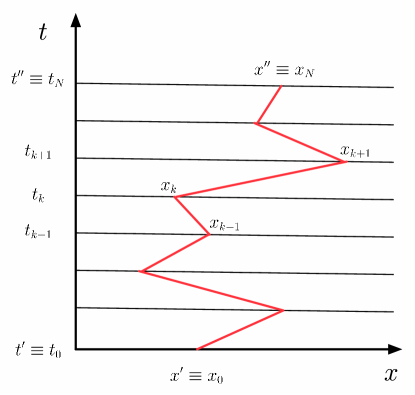
Figure 2.1: Illustration of the path integral for a one-dimensional non-relativistic quantum mechanical problem, e.g. a propagating particle. One possible path of the configuration space (path space) is drawn. The “virtual” particle is propagating from $x_{0}$ to $x_{N}$ in a piecewise linear path of N steps of time $\epsilon=(t^{\prime\prime}-t^{\prime})/N$ each.

The evaluation of the path integral now amounts to computing $N$ integrals of the following form,

$$G(x,t;x^{\prime},t^{\prime})=\lim_{\epsilon\rightarrow 0}A^{-N}\prod_{k=1}^{N-1}\int dx_{k}\exp\left\{i\sum_{j=0}^{N-1}S(x_{j+1}-x_{j})\right\}.$$ (2.17)

Note that this integral is not well defined, since the integrand is a complex valued phase factor. To be able to compute the integral one has to analytically continue the time variable $t\rightarrow\tau=it$. This so-called Wick rotation converts the path integral into a set of real gaussian integrals that can be performed to obtain the regularized Euclidean amplitude. The continuum amplitude can now be computed by taking the limit where the time intervals become infinitesimally small, $\epsilon\rightarrow 0$. Notice that in this limit the velocity and therefore the extrinsic geometry becomes singular at each point of a typical trajectory in the path integral. In other words, the typical paths that contribute to the path integral are highly non-differentiable. Similarly, the intrinsic geometry will typically also be singular if one defines a gravitational path integral by dynamical triangulations. After taking the continuum limit one can obtain the physical Lorentzian amplitude by applying the inverse Wick rotation $\tau\rightarrow\tau=-it$.

Notice that in this form the Wick rotation is an analytic continuation in the coordinate $t$ implying that this procedure is not invariant under coordinate transformations. Taking a gravitational viewpoint, one might ask the question whether it is possible to define a Wick rotation for point particles that does not involve coordinates? In the following we suggest that it is indeed possible to construct a Wick rotation for a point particle that is independent of the particular background and coordinate system.

2.5.2 The invariant Wick rotation for particles

We start by considering the standard action principle for the massive relativistic point particle. The action is well known and simply proportional to the invariant length of the four dimensional wordline,

$$S=-m\int ds,$$ (2.18)

where the invariant length is given as usual by

$$ds^{2}=-g_{\mu\nu}(x)dx^{\mu}dx^{\nu}.$$ (2.19)

Suppose that a classical trajectory is written as $x^{\mu}(\tau)$, where $\tau$ is an arbitrary coordinate that labels the points along the worldline. Then the action may be written in the familiar form

$$S=-m\int d\tau\sqrt{-\dot{x}^{2}}.$$ (2.20)

This action has the very important property that it is invariant under both four dimensional coordinate transformations and reparameterizations of the coordinate on the worldline. Thus it really describes the extrinsic geometry of the worldline as it is embedded in the ambient space and not some particular choice of coordinates. The action has its shortcomings however, since it has a complicated square root dependence and is not valid for massless particles. These difficulties can be overcome by introducing a one dimensional einbein on the worldline. In terms of the einbein the action for a point particle can be written in the following form

$$S=-\frac{1}{2}\int\left(e^{-2}\dot{x}^{2}-m^{2}\right)e\>d\tau.$$ (2.21)

Solving the equation of motion for the einbein gives

$$\dot{x}^{2}+e^{2}m^{2}=0.$$ (2.22)

Substituting this result back in (2.21) one recovers the action (2.20). The here described relation between the two point particle actions (2.20) and (2.21) is completely analogous to the relation between the Nambu Goto and the Polyakov string actions respectively. One way to view the einbein is that it is just the lapse function of the one dimensional geometry along the worldline, since the einbein has just a single component. Essentially, the action (2.21) describes the physics of a point particle as one dimensional quantum gravity coupled to the coordinates and metric of the target space. Now we are in a position to define the coordinate and background independent Wick rotation for the point particle. If we introduce the signature constant $\varsigma$ for both the lapse function of the target space and the lapse function of the worldline we obtain the following action,

$$S=\frac{1}{2}\int\left(\frac{\dot{x}^{2}}{\varsigma e^{2}}+m^{2}\right)\sqrt{-\varsigma}e\>d\tau,$$ (2.23)

where

$$\dot{x}^{2}=\varsigma N^{2}\dot{t}^{2}+2S_{\sigma}\dot{t}\dot{x}^{\sigma}+h_{\sigma\rho}\dot{x}^{\sigma}\dot{x}^{\rho}.$$ (2.24)

From (2.23) and (2.24) it is now easily seen that the Lorentzian action is rotated to $i$ times the Euclidean action when $\varsigma$ is analytically continued from $-1$ to $+1$.

2.5.3 Quantum gravity from simplicial intrinsic geometry

As motivated in section (2.5.1), regularization by lattice methods can be a powerful tool to define and evaluate geometrical path integrals. In the example of the point particle the path integral is evaluated with the help of a discretization of its extrinsic geometry. Similar to the point particle, quantum gravity is a quantum theory of geometry, yet unlike the quantum particle it is the intrinsic geometry that plays a central role. So the strategy of causal dynamical triangulations to formulate a path integral for quantum gravity is to employ a suitable discretization for the intrinsic properties of the space of geometries.

Figure 2.2: A patch of flat space represented by a regular triangulation

Discrete methods have had a long tradition in geometry and are a natural tool in the study of the gravitational dynamics. Notably, Regge [12] discussed that the intrinsic geometry of a manifold can be discretized by piecewise flat geometries. In arbitrary dimensions a general piecewise flat geometry consists of flat building blocks called polytopes. These polytopes are the natural generalizations of polygons (d=2) and polyhedra (d=3). Often the piecewise flat geometries are constructed solely from elementary polytopes known as simplices. A simplex is the higher dimensional generalization of a triangle, in any dimension it is the polytope with the minimal number of boundary components. In principle a discrete manifold that is constructed purely from simplices is called a simplicial manifold. Often however such geometries are simply referred to as triangulations. These triangulations can be thought of as a straightforward analogue of the piecewise linear trajectories that appear in the construction of the path integral for the point particle.

One of the benefits of using a simplicial geometry to approximate an arbitrary manifold is that the metric properties are completely fixed by specifying all edge lengths. From the metric information one can extract the local curvature which is the relevant object when considering gravitational dynamics. The notion of curvature for simplicial manifolds was found initially by Regge [12] and was later refined in [40]. The prime focus of this work is on two dimensional quantum gravity, so we explain the Regge curvature in this simple setting.

A simple way to understand the Regge curvature is to first consider a regular triangulation of equilateral triangles (fig. 2.2). Such a triangulation is a proper simplicial representation of an everywhere flat manifold. This can be seen by noticing that each vertex is associated with precisely $6$ triangles. Furthermore, the triangles are equilateral implying that the angle between its sides is $\tfrac{1}{3}\pi$. So we can conclude that the total angle around each point is equal to $2\pi$ as should be for a flat manifold. Introducing local curvature deformations can now be done in two different ways. Historically, the preferred approach is to deform the triangles by altering the length of the edges. Applying such a deformation to one of the edges of the flat triangulation causes the total angle around its vertices to be different from $2\pi$. Since all triangles are still constrained to be flat this implies that conical singularities are introduced by the deformation. The amount by which the total angle around a vertex differs from $2\pi$ is called the deficit angle $\epsilon_{v}=2\pi-\sum_{i\supset v}\theta_{i}$. The scalar curvature of a vertex can now be directly related to this deficit angle by invoking the concept of the so-called dual lattice, namely

Figure 2.3: A section of a triangulation and its dual graph

$$R_{v}=2\frac{\epsilon_{v}}{V_{v}},$$ (2.25)

where $V_{v}$ is the volume of a cell of the dual lattice. Each triangulation has a unique dual lattice that is easily constructed by connecting the “barycenters” of the triangles with edges of the dual lattice (fig. 2.3). The relation between the scalar curvature and the deficit angle is defined by parallel transporting a vector along the edges of the dual lattice that encompass the vertex under consideration. The curvature is proportional to the angle by which the vector is rotated after one full encircling of the cell of the dual lattice. The result is given by (2.25), the angle by which a vector is rotated after one revolution along the dual lattice is proportional to the strength of the conical singularity and inversely proportional to the volume of the cells of the dual lattice.

So the curvature of a geometry which is discretized according to the prescription of Regge is given by a set of Dirac delta functions located at the vertices of the triangulation. The distributional character of the curvature is very similar to the non differential behavior of the histories in the path integral of the point particle and related to the distributional properties of quantum fields in general.

Given the above notion of curvature it is straightforward to introduce the discrete equivalent of the Einstein Hilbert action, called the Regge action,

$$S_{\mathrm{Regge}}=\sum_{v}V_{v}\left(\lambda-k\,\frac{\epsilon_{v}}{V_{v}}\right).$$ (2.26)

Observe that this discrete action is manifestly independent of any coordinates as is promised by the title of [12]. Originally this discrete formulation of the gravitational action was conceived as a useful tool to study classical aspects of general relativity. It was proposed that the gravitational dynamics could be conveniently studied by varying the length of the edges of the simplicial manifold. This approach to simplicial gravity is called Regge calculus. In its classical incarnation it has had some success but the interest particularly gained impetus with the proposition that it might serve as a convenient platform for constructing a quantum theory of gravity [14] [41]. The main idea is to use the Regge action to construct a path integral over the edge lengths of a simplicial manifold with fixed connectivity. The approach is succinctly called Quantum Regge calculus, since it is a rather faithful generalization of Regge calculus to the quantum domain.

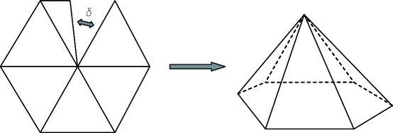
Figure 2.4: A positive deficit angle created by deforming a triangle

Quantum Regge calculus has not been able give us much understanding beyond semiclassical gravity however. In the context of two dimensional gravity some doubts have been raised about the consistency of the approach [42]. One of the objections is that the approach is not able to reproduce results from other methods such as Liouville field theory or dynamical triangulations.

In [43] it was proposed that although the formalism of Regge calculus is free of coordinates it is not completely gauge invariant. According to their point of view it is possible to perform such a gauge fixing, but the associated Faddeev-Popov determinants generate a highly non-local measure which makes the theory very hard to handle.

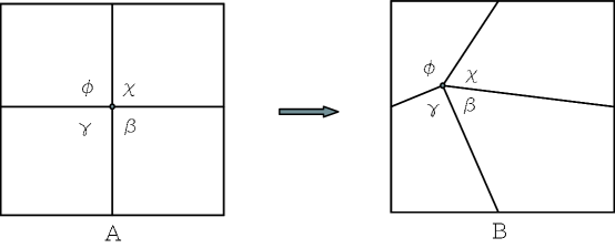
Figure 2.5: All discretizations for which $\phi+\chi+\beta+\gamma=2\pi$ represent the same flat geometry.

An insightful way to visualize the possible overcounting problems in Regge calculus, at least in two dimensions, is to consider the discretization of a flat two dimensional manifold in terms of four squares (fig. 2.5). If the squares are equilateral it is clear that the total angle around the central vertex is $2\pi$, hence the manifold is flat everywhere also at the central vertex. If we allow the edges connecting the vertex to fluctuate there still are some possibilities that keep the manifold flat. Basically, the fluctuations of the edges that keep the total angle around the central vertex fixed at $2\pi$ might be considered “gauge transformations”, since they do not alter the intrinsic geometry of the manifold. In this context it is interesting to notice that the Regge action only depends on the total angle around a vertex and not on the angles of individual simplices. One might however argue, that the overcounting problems only appear when one discretizes manifolds with a high degree of symmetry, such as flat space. Moreover, in the path integral these special geometries are typically of “measure zero” which implies that the overcounting issue is only a minor problem.

2.5.4 Dynamical triangulations

To ameliorate the technical issues of the Regge calculus program, the method of dynamical triangulations was developed. Similar to Regge calculus the scheme is free of coordinates, since both methods are based on the Regge action. The crucial difference however, is that in dynamical triangulations the length of all edges in the triangulations are fixed and the geometry is encoded in the nontrivial gluing of the simplices. So instead of altering the edge lengths one introduces curvature by adding or removing simplices (see fig. 2.6). An indication that this method does not lead to overcounting problems in simple situations is that the simplicial representation of a given flat manifold is unique. In addition, adding or removing a triangle always changes the physical curvature and volume of the geometry, implying that also in more complicated situations the discretization seems to be free of overcounting problems. Although dynamical triangulation methods are not very efficient to approximate individual classical geometries, they are ideally suited for a discretization of geometries as histories in a path integral for quantum gravity.

The dynamical triangulation approach to quantum gravity was initially introduced in the context of two dimensional Euclidean quantum gravity [44, 45, 46] where it turned out to be a very powerful technique to explicitly compute the continuum amplitudes for Euclidean quantum gravity. Contrary to the usual situation, the discrete approach of dynamical triangulations is often more powerful than continuum methods. Many amplitudes can be obtained with ease and the procedure is considerably more straightforward than the computation of the amplitudes from the corresponding continuum Liouville field theory. Actually, the quantization of Liouville theory only gained considerable impetus about $15$ years later in the seminal work [19]. Although the results do not yet cover all aspects of quantum Liouville theory, it is an important contribution to the quantization of two dimensional gravity. Another example of the strength of the dynamical triangulation method is that the results for the amplitudes for Euclidean manifolds of arbitrary genus are exclusive to this method [47, 48].

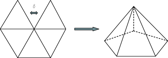
Figure 2.6: A positive deficit angle created by removing a triangle

So the approach of dynamical triangulations is proven to be a useful tool to study Euclidean quantum gravity. It turns out however that if one studies the quantum geometry of two dimensional quantum gravity it does not behave as we might expect from a “realistic” quantum theory of gravity. Not even the dimension of geometry is what it is supposed to be, the Hausdorff dimension of the quantum geometry is four and not two. The principle cause of this behavior comes from the domination of cutoff scale outgrowths in the path integral. In chapter 3 we analyze the properties of the quantum geometry of two dimensional Euclidean quantum gravity in some detail.

Since the results of the dynamical triangulation scheme can be compared with continuum calculations, one concludes that the fractal structure of the geometry is not a consequence of the triangulation method, but an intrinsic property of two dimensional Euclidean quantum gravity. The initial attitude was that the somewhat degenerate behavior of the quantum geometry is due to the simplicity of two dimensional gravity. Therefore, higher dimensional versions of the dynamical triangulation model were developed and investigated by means of computer simulations, see [49] and [50] for the three dimensional model and [51, 52] for the four dimensional model.

The hope that the higher dimensional models might be better behaved than the two dimensional model did not materialize though. It was found that in the infinite volume limit these higher dimensional dynamical triangulation models have two phases, a crumpled phase where the Hausdorff dimension is very large and a tree like phase where the geometry resembles a branched polymer. Both phases are not satisfactory from a physical point of view, so a suitable continuum limit is not automatically reached in either phase. Nonetheless, one of the initial ideas was that an appropriate continuum limit perhaps exists at the critical point separating the crumpled and branched polymer phases. Subsequent analysis revealed those hopes to be in vain as it was shown that even in the four dimensional model the phase transition is of first order [53, 54].

An important lesson that can be learned from these investigations is the following, if one constructs a random geometry model based on simplices of a certain dimension one is not at all assured that the quantum geometry behaves anything like a manifold of that dimension.

2.6 2D causal dynamical triangulations

In this section we introduce the concept of causal dynamical triangulations. The motivation behind the inception of causal dynamical triangulations was twofold:

1. The quantum geometry of four dimensional Euclidean dynamical triangulation models seem incompatible with a well behaved continuum limit.
   

2. The Lorentzian signature of the spacetimes should be taken seriously.

To address the Lorentzian nature of the path integral it is of paramount importance to have an intrinsically defined notion of time. In causal dynamical triangulations this problem is addressed by studying piecewise linear geometries that have a layered structure. The layered structure of the triangulations allows one to globally distinguish timelike and spacelike edges. Furthermore, the global foliation of the discrete geometries allows one to define a consistent Wick rotation.

The central amplitude one aims to compute in two dimensional causal dynamical triangulations is the so-called cylinder amplitude or causal propagator. This quantity describes the probability amplitude for a quantum ensemble of two dimensional geometries of Lorentzian signature with an initial and a final boundary, where every point of the initial boundary has the same timelike geodesic distance to the final boundary. In two dimensions the boundaries are one dimensional curves with the topology of a $S^{1}$ so the only information that characterizes the intrinsic geometry of the boundaries is their length.

The strategy of causal dynamical triangulations is to discretize the manifolds in the path integral with flat triangles. These Minkowski triangles have one spacelike edge satisfying $L_{s}^{2}=+a^{2}$ and two timelike edges with $L_{\tau}^{2}=-a^{2}$. By construction, one chooses spacetimes which consist of $T/a$ strips with the topology of $S^{1}\times[0,1]$, where the timelike height of the strip is proportional to $a$. Each strip has two spatial boundaries, one spatial section at time $\tau$ with length $L(\tau)=al_{t}$ and one at time $\tau+a$ with length $L(\tau+a)=al_{t+1}$. The geometry of a general circular strip is now determined by the ordering of $l_{t+1}$ triangles “pointing up” and $l_{t}$ triangles “pointing down” as illustrated in fig. 2.7.

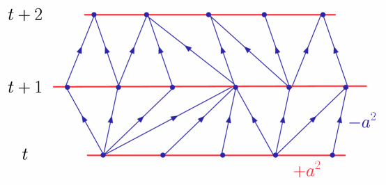
Figure 2.7: Section of a 2d Lorentzian triangulation consisting of spacetime strips of height $\Delta t\!=\!1$. Each spatial slice is periodically identified, such that the simplicial manifold has topology $[0,1]\!\times\!S^{1}$. One sees that a single strip with lower boundary length $l_{t}$ and upper boundary length $l_{t+1}$ consists exactly of $l_{t}$ up pointing triangles and $l_{t+1}$ down pointing triangles.

Since the triangles are genuine patches of flat Minkowski space, they are naturally equipped with a local light cone structure. Furthermore, from the global distinction between timelike and spacelike edges one sees that the triangulation equips the manifold with a global causal structure. By virtue of this global causal structure it is possible to define a Wick rotation for curved manifolds. In the triangulation context the Wick rotation amounts to changing the squared length of the timelike edges from negative to positive signature $L_{\tau}^{2}=-a^{2}\mapsto L_{\tau}^{2}=a^{2}$. As in the continuum case this rotation should be treated with some care and one must show that the Lorentzian action defined with $L_{\tau}^{2}=-a^{2}$ and the Euclidean action with $L_{\tau}^{2}=a^{2}$ can be connected by a smooth deformation. In appendix A we discuss the Regge action for these two dimensional Minkowski triangulations. It is shown that the Lorentzian and the Euclidean Regge action, multiplied with the imaginary unit $i$, are indeed connected by a smooth analytical continuation of the parameter $\alpha$ from $-1$ to $1$ where $\alpha$ is defined by $L_{\tau}^{2}=\alpha a^{2}$. So the Wick rotation indeed possesses the desired property that the weight in the path integral is converted from a complex phase factor to a real Boltzmann type weight.

$$\mathcal{W}:\quad e^{i\,S_{\mathrm{Regge}}(T^{lor})}\mapsto e^{-\,S_{\mathrm{Regge}}(T^{eu})}.$$ (2.27)

As we shall see in the forthcoming section the above defined kinematical structures reduce the computation of the path integral for the causal propagator to a statistical mechanics problem.

2.7 The discrete solution

The basic ingredients of any statistical model are the entropy and the Boltzmann weight. For the two dimensional causal dynamical triangulations model the entropy is generated by the number of geometrically distinct ways one can organize the Minkowski triangles in a layered structure as depicted in fig. 2.7. The Boltzmann factor on the other hand is related to the Regge action associated to the triangles. In two dimensions the Regge action is particularly simple, since the two dimensional Einstein-Hilbert term is a topological invariant.

$$\int_{M}d^{2}x\sqrt{|\det g|}\,R(x)=2\pi\chi(M),$$ (2.28)

where $\chi(M)\!=\!2\!-\!2{\mathfrak{g}}-b$ is the Euler characteristic of the manifold $M$, ${\mathfrak{g}}$ is the genus and $b$ is the number of boundary components of the manifold. For the moment we fix the topology of the manifold to be of the form $S^{1}\times[0,1]$. This choice corresponds to what we refer to as “bare”or equivalently “pure” causal dynamical triangulation model as originally introduced by Ambjørn and Loll in [21]. One of the new contributions of this thesis is that we go beyond the assumption of fixed topology and in chapter 3 we introduce a model where controlled spatial topology changes are an integral part of the quantum geometry. For such models the Einstein-Hilbert part of the action is essential as it tames the topology changes by introducing a Boltzmann weight that suppresses manifolds with complicated topology in the path integral. Since the topology is fixed in the pure model the Einstein-Hilbert action can act at most as an overall phase factor in the path integral. Furthermore, for the pure causal dynamical triangulations model we are solely interested in manifolds with the topology of a cylinder so the Euler characteristic is zero, making Newton’s constant irrelevant for two dimensional quantum gravity without topology change.

The only quantity which is relevant for the dynamics of the pure dynamical triangulation model is the total volume of the manifold. The Regge action is then simply proportional to the added volume of all triangles of a specific configuration,

$$S_{\mathrm{Regge}}(T)=\tilde{\lambda}\,a^{2}\,N(T),$$ (2.29)

where $\tilde{\lambda}$ is the bare cosmological constant and $N(T)$ the number of triangles in the triangulation $T$. Note that an order one factor coming from the volume term has been absorbed into $\tilde{\lambda}$. The path integral for the propagator can now be written as follows

$$G_{\tilde{\lambda}}(l_{1},l_{2};t)=\sum_{\mathcal{T}}\frac{1}{C_{\mathcal{T}}}\>\>e^{i\,\tilde{\lambda}\,a^{2}\,N(T)},$$ (2.30)

where $\mathcal{T}$ denotes the causal triangulations with initial boundary length $l_{1}$ and final boundary length $l_{2}$, and $C_{\mathcal{T}}$ denotes the volume of the automorphism group of a triangulation. Basically it is the symmetry factor of the manifold that is still left after factoring out the diffeomorphisms. After a Wick rotation the discrete sum over quantum amplitudes is converted to a genuine statistical model with a real Boltzmann weight,

$$G_{\lambda}(l_{1},l_{2};t)=\sum_{\mathcal{T}}\frac{1}{C_{\mathcal{T}}}\>\>e^{-\lambda\,a^{2}\,N(T)},$$ (2.31)

where it should be noted that $\lambda$ and $\tilde{\lambda}$ differ by an order one constant because of the different volume of Minkowskian and Euclidean triangles (see appendix A). The layered structure of the triangulations has the natural implication that the propagator satisfies the following semi-group property or composition law,

$$G_{\lambda}(l_{1},l_{2};t_{1}+t_{2})=\sum_{l}l\>G_{\lambda}(l_{1},l;t_{1})\;G_{\lambda}(l,l_{2};t_{2}).$$ (2.32)

The measure factor $l$ in the composition law comes from the circular nature of a strip. Writing the composition law for $t_{1}=1$ we see that the one step propagator acts as a transfer matrix,

$$G_{\lambda}(l_{1},l_{2};t+1)=\sum_{l}l\>G_{\lambda}(l_{1},l;1)\;G_{\lambda}(l,l_{2};t).$$ (2.33)

In the following we derive $G_{\lambda}(l_{1},l_{2};t)$ by iterating (2.33) $t$ times. The iteration procedure can be conveniently carried out by introducing the generating function for $G_{\lambda}(l_{1},l_{2};t)$

$$G_{\lambda}(x,y;t)\equiv\sum_{k,l}x^{k}\,y^{l}\;G_{\lambda}(k,l;t),$$ (2.34)

where $x$ and $y$ can be naturally interpreted as Boltzmann weights related to the boundary cosmological constants of individual triangles,

$$x=\mbox{e}^{-\lambda_{i}a},\leavevmode\nobreak\ \leavevmode\nobreak\ \leavevmode\nobreak\ \leavevmode\nobreak\ y=\mbox{e}^{-\lambda_{o}a}.$$ (2.35)

Analogously we write the Boltzmann weight related to the bulk cosmological constant as follows,

$$g=\mbox{e}^{-\lambda a^{2}}.$$ (2.36)

The above introduced notation implies that the total Boltzmann weight of one strip can be determined by associating a factor of $gx$ with triangles that have the spacelike edges on the entrance loop and a factor $gy$ to triangles where the spacelike edges are on the exit loop. The one step propagator is now easily computed by standard generating function techniques as follows,

$$G(x,y;g;1) = \raisebox{-10.0pt}{\includegraphics[height=25.0pt]{route1}}+\raisebox{-10.0pt}{\includegraphics[height=25.0pt]{route2}}+\raisebox{-10.0pt}{\includegraphics[height=25.0pt]{route3}}+...$$ (2.37)

$$= \sum^{\infty}_{k=1}\frac{1}{k}\left(\sum^{\infty}_{m=1}(gx)^{m}\sum^{\infty}_{n=1}(gy)^{n}\right)^{k},$$

where the factor $\tfrac{1}{k}$ comes from dividing by the volume of the automorphism group for periodic triangulations. Evaluating the summations in (2.37) we readily obtain

$$G(x,y;g;1)=\sum^{\infty}_{k=1}\frac{1}{k}\left(\frac{gx}{1-gx}\frac{gy}{1-gy}\right)^{k}=-\log\left(1-\frac{gxgy}{(1-gx)(1-gy)}\right).$$ (2.38)

From this expression it can be seen that the one step propagator with fixed boundary lengths is given by

$$G(l_{1},l_{2};g;1)=g^{l_{1}+l_{2}}\frac{1}{l_{1}+l_{2}}\binom{l_{1}+l_{2}}{l_{1}},$$ (2.39)

where the division by the volume of the automorphism group now makes its appearance in the guise of the factor $\tfrac{1}{l_{1}+l_{2}}$.

To compute the “finite time propagator” $G(x,y;g;t)$, we rewrite the composition law (2.32) in terms of generating functions and obtain the following,

$$G(x,y;g;t_{1}+t_{2})=\oint\oint\frac{dz}{2\pi i}\>\frac{dz^{\prime}}{2\pi i}\>\frac{1}{\left(1-zz^{\prime}\right)^{2}}\>G(x,z;g;t_{1})G(z^{\prime},y;g;t_{2}).$$ (2.40)

By setting $t_{2}=1$ and performing the contour integration over $z$ we obtain

$$G(x,y;g;t)=\oint\frac{dz^{\prime}}{2\pi iz^{\prime 2}}\>\left[\frac{d}{dz}G_{\lambda}(x,z;1)\right]_{z=1/z^{\prime}}G_{\lambda}(z^{\prime},y;t-1).$$ (2.41)

Inserting the expression for the one step propagator yields the desired iterative equation for $G(x,y;g;t)$,

$$G(x,y;g;t)=G\left(\frac{g}{1-gx},y;g;t-1\right)-G_{\lambda}\left(g,y;g;t-1\right).$$ (2.42)

The implicit solution of this equation can be written as

$$G(x,y;g;t)=\log\left(\frac{1}{1-F_{t}(x)y}\right)-\log\left(\frac{1}{1-F_{t-1}(g)y}\right),$$ (2.43)

where $F_{t}$ is defined iteratively by

$$F_{t}(x)=\frac{g}{1-gF_{t-1}(x)},\leavevmode\nobreak\ \leavevmode\nobreak\ \leavevmode\nobreak\ \leavevmode\nobreak\ F_{0}(x)=x.$$ (2.44)

The fixed point $F$ as defined by $F_{t}(x)=F_{t-1}(x)$ is given by

$$F=\frac{1-\sqrt{1-4g^{2}}}{2g},\leavevmode\nobreak\ \leavevmode\nobreak\ \leavevmode\nobreak\ \leavevmode\nobreak\ g=\frac{1}{F+1/F}.$$ (2.45)

By well known methods one can use the fixed point to find the explicit solution to the iterative equation (2.44)

$$F_{t}(x)=\frac{B_{t}-xC_{t}}{A_{t}-xB_{t}},\leavevmode\nobreak\ \leavevmode\nobreak\ \leavevmode\nobreak\ \leavevmode\nobreak\ F_{t-1}\left({\textstyle{g}}\right)=\frac{B_{t}}{A_{t}},$$ (2.46)

where

$$A_{t}=1-F^{2t+2},\leavevmode\nobreak\ \leavevmode\nobreak\ \leavevmode\nobreak\ B_{t}=F-F^{2t+1},\leavevmode\nobreak\ \leavevmode\nobreak\ \leavevmode\nobreak\ C_{t}=F^{2}-F^{2t}.$$ (2.47)

The complete finite time propagator is now obtained by substituting (2.46) in (2.43), yielding

$$G(x,y;g;t)=-\log\left(1-Z(x,y;g;t)\right),$$ (2.48)

where we have defined

$$Z(x,y;g;t)={\textstyle\left(1-\frac{A_{t}C_{t}}{B_{t}^{2}}\right)}\frac{\frac{B_{t}}{A_{t}}x\frac{B_{t}}{A_{t}}y}{\left(1-\frac{B_{t}}{A_{t}}x\right)\left(1-\frac{B_{t}}{A_{t}}y\right)}.$$ (2.49)

The region of convergence of this result as an expansion in powers of $x,y,z$ is

$$|g|<\frac{1}{2},\quad|x|<1,\quad|y|<1.$$ (2.50)

2.7.1 The continuum limit

One of the central philosophies behind the method of dynamical triangulations is “universality”. This concept is well known in statistical mechanics and plays a pivotal role in renormalization theory. As applied to the case at hand it means that the precise form of the discrete amplitude (2.48) should not be important for the physics of the system. The essential physics should for example not depend on the type of polytopes that are used to regularize the path integral.

One of the prerequisites for such a scenario is that there exists a so-called “critical” hypersurface in the space of parameters of the regularized theory. Near such a region the theory exhibits correlations that are much larger than the size of the building blocks. If this happens the macroscopic physics is insensitive to the regularization and one can safely take the limit where the building blocks are infinitesimally small and obtain a more or less unique continuum theory.

Precisely how the above sketched scenario is realized in two dimensional causal dynamical triangulations can be most easily understood by analyzing the one step propagator as a function of $g,x,y$. To identify the critical surface in the parameter space spanned by the three couplings $g$,$x$ and $y$ we compute the average number of triangles in one strip. This can be readily accomplished by taking the derivative with respect to $g$ of the one step propagator since $g$ can be seen as the fugacity for the number of triangles in the system,

$$\langle N_{\bigtriangleup}\rangle=g\frac{d}{dg}G(x,y;g;1)=1-\frac{1}{1-gx}-\frac{1}{1-gy}+\frac{1}{1-g(x+y)}.$$ (2.51)

The critical region of the parameter space can now easily be identified by observing that the total number of building blocks diverges if the couplings satisfy the following relation,

$$|g(x+y)|=1,$$ (2.52)

where it should be noted that besides this relation the couplings are also subject to the convergence condition (2.50). Near the critical region (2.52) the typical length scale of the system is indeed much larger than the length scale of the individual building blocks. To define the continuum limit of the theory we assume canonical scaling dimensions for the bulk and boundary cosmological constants,

$$g=g_{c}e^{-a^{2}\Lambda},\quad x=x_{c}e^{-aX},\quad y=y_{c}e^{-aY}.$$ (2.53)

Since we have performed the Wick rotation one is dealing with real valued $g,x,y$. Therefore the natural critical values for these couplings are determined by (2.50) and (2.52) yielding

$$g_{c}=1/2,\leavevmode\nobreak\ \leavevmode\nobreak\ \leavevmode\nobreak\ \leavevmode\nobreak\ x_{c}=1,\leavevmode\nobreak\ \leavevmode\nobreak\ \leavevmode\nobreak\ \leavevmode\nobreak\ y_{c}=1,$$ (2.54)

leading to the following scaling relations,

$$g=\frac{1}{2}e^{-a^{2}\Lambda},\quad x=e^{-aX},\quad y=e^{-aY}.$$ (2.55)

The continuum limit of the propagator can now be determined uniquely by inserting the scaling relations (2.55) into the regularized result (2.48), giving

$$G_{\Lambda}(X,Y,T)=-\log\left(1-Z_{\Lambda}(X,Y,T)\right),$$ (2.56)

where

$$Z_{\Lambda}(X,Y,T)=\frac{\Lambda}{(X+\sqrt{\Lambda}\coth\sqrt{\Lambda}T)(Y+\sqrt{\Lambda}\coth\sqrt{\Lambda}T)}.$$ (2.57)

Note that in the continuum limit we defined the normalization of the wavefunctions such that

$$G_{\Lambda}(X,Y,T)=aG(x,y;g;t).$$ (2.58)

The power of $a$ is uniquely determined by the requirement that the continuum propagator satisfies a continuum analogue of the composition law (2.40). The continuum expression for the propagator where the boundary lengths are fixed instead of the boundary cosmological constants can now be obtained by an inverse Laplace transformation of (2.56) with respect to both $X$ and $Y$,

$$G_{\Lambda}(L_{1},L_{2};T)=\frac{\mbox{e}^{-\sqrt{\Lambda}\coth\sqrt{\Lambda}T(L_{1}+L_{2})}}{\sinh\sqrt{\Lambda}T}\;\frac{\sqrt{\Lambda}}{\sqrt{L_{1}L_{2}}}\;\;I_{1}\left(\frac{2\sqrt{\Lambda L_{1}L_{2}}}{\sinh\sqrt{\Lambda}T}\right),$$ (2.59)

where $I_{1}(x)$ is a modified Bessel function of the first kind. One indication that this object is a good propagator is that it satisfies the expected composition law

$$G_{\Lambda}(L_{1},L_{2};T_{1}+T_{2})=\int_{0}^{\infty}\mbox{d}L\,L\;G_{\Lambda}(L_{1},L;T_{1})\,G_{\Lambda}(L,L_{2},T_{2}).$$ (2.60)

From the propagator one can naturally define the time dependent disc function by shrinking one of the boundary loops to zero,

$$W_{\Lambda}(L,T)=G_{\Lambda}(L,L^{\prime}\!=\!0;T),$$ (2.61)

with

$$G_{\Lambda}(L,L^{\prime}\!=\!0;T)=\frac{\Lambda}{\sinh^{2}\sqrt{\Lambda}T}e^{{-\sqrt{\Lambda}L\coth\sqrt{\Lambda}T}}.$$ (2.62)

This object could be given a cosmological interpretation in that it is the probability amplitude to find a universe of size $L$ that has existed for a time $T$. Upon doing an integration over time one obtains an object that has the natural interpretation of a Hartle Hawking wavefunction,

$$W_{\Lambda}(L)=\int_{0}^{\infty}dT\;W_{\Lambda}(L,T)=\frac{e^{-\sqrt{\Lambda}L}}{L}.$$ (2.63)

Alternatively, this object is often called the disc function.

2.7.2 Marking the causal propagator

In most expositions on two dimensional causal dynamical triangulations the conventions differ from the ones used in the previous section. Often, one employs propagators that have a marked vertex on the initial boundary,

$$G^{(1;0)}_{\lambda}(l_{1},l_{2};1)=l_{1}G_{\lambda}(l_{1},l_{2};1),$$ (2.64)

where the superscript notation $G^{(1;0)}$ denotes that the entrance loop of the propagator is marked, $G^{(0;1)}$ implies that the exit loop is marked and $G^{(1;1)}$ means that both loops are marked. In principle all vertices of the triangulation are indistinguishable, the introduction of a mark on the boundary implies that one vertex on the boundary is distinguishable from all others. The main virtue of the marking is that it removes the measure factor in the composition law for the propagator (2.32)

$$G^{(1;0)}_{\lambda}(l_{1},l_{2};t_{1}+t_{2})=\sum_{l}G^{(1;0)}_{\lambda}(l_{1},l;t_{1})\;G^{(1;0)}_{\lambda}(l,l_{2};t_{2}),$$ (2.65)

which corresponds to the following composition law for the Laplace transformed propagator,

$$G^{(1;0)}_{\lambda}(x,y;t_{1}+t_{2})=\oint\frac{dz}{2\pi i\,z}\;G^{(1;0)}_{\lambda}(x,z^{-1};t_{1})G^{(1;0)}_{\lambda}(z,y;t_{2}).$$ (2.66)

Many formulas simplify with this trick, but the price one pays is that the propagator is no longer symmetric. Although the physical symmetry of the two boundary components of the causal propagator is not reflected in the marked expressions we discuss their properties for future convenience.

Since we have already computed the one step propagator without a mark, we can find the marked version by simply taking a derivative with respect to the boundary cosmological constant,

$$G^{(1;0)}(x,y;g;1)=x\frac{d}{dx}G^{(1;0)}_{\lambda}(x,y;g;1)=\frac{g^{2}xy}{(1-gx)(1-g(x+y))}.$$ (2.67)

To find the marked propagator for finite $t$ one can find an iterative equation analogous to (2.42) ,

$$G^{(1;0)}(x,y;g;t)=\frac{gx}{1-gx}\;G^{(1;0)}\left(\frac{g}{1-gx},y;g;t-1\right).$$ (2.68)

Evidently, one can use this relation in a similar iteration procedure as described in section (2.7) to obtain $G^{(1,0)}(x,y;g;t)$ and then apply the scaling relations to find the continuum propagator. Instead, one can also apply the scaling relations (2.55) directly to (2.68) and find a differential equation for the continuum marked propagator,

$$\frac{\partial}{\partial T}G^{(1;0)}_{\Lambda}(X,Y,T)=-\frac{\partial}{\partial X}\left[{\hat{W}}(X)G^{(1;0)}_{\Lambda}(X,Y,T)\right],$$ (2.69)

where

$${\hat{W}}(X)=X^{2}-\Lambda.$$ (2.70)

The notation ${\hat{W}}(X)$ is introduced to anticipate generalizations, since this differential equation can also be solved for more general expressions than (2.70). Equation (2.69) has the form of a standard first order differential equation, so to solve it uniquely one needs to supply one boundary condition. The natural condition to impose on the propagator is that it reduces to the identity for the limit of zero proper time $T$,

$$G^{(1;0)}_{\Lambda}(L_{1},L_{2};T\!=\!0)=\delta(L_{1}-L_{2}),$$ (2.71)

which has the following analogue in terms of boundary cosmological constants,

$$G^{(1;0)}_{\Lambda}(X,Y;T\!=\!0)=\frac{1}{X+Y}.$$ (2.72)

Solving the differential equation (2.69) with this boundary condition gives

$$G^{(1;0)}_{\Lambda}(X,Y,T)=\frac{{\hat{W}}({\bar{X}}(T))}{{\hat{W}}(X)}\frac{1}{{\bar{X}}(T)+Y},$$ (2.73)

where $\bar{X}(T;X)$ is the solution to the characteristic equation

$$\frac{d{\bar{X}}}{dT}=-{\hat{W}}({\bar{X}}(T)),\quad{\bar{X}}(T=0)=X.$$ (2.74)

Since here we are interested in pure CDT, the definite form of this equation is known since ${\hat{W}}(X)=X^{2}-\Lambda$ and one can solve the characteristic equation explicitly,

$$\bar{X}(T)=\sqrt{\Lambda}\;\frac{(\sqrt{\Lambda}+X)-\mbox{e}^{-2\sqrt{\Lambda}T}(\sqrt{\Lambda}-X)}{(\sqrt{\Lambda}+X)+\mbox{e}^{-2\sqrt{\Lambda}T}(\sqrt{\Lambda}-X)}.$$ (2.75)

Inserting this expression in (2.73) it is easily verified that this form of the propagator is fully compatible with the previously derived results. If one marks the unmarked propagator (2.56) by taking a derivative with respect to the initial boundary cosmology constant $X$, the expression coincides precisely with the above derived result (2.73) .

2.7.3 Hamiltonians in causal quantum gravity

An interesting observation regarding the differential equation for the causal propagator (2.69) is that it can be viewed as a Wick rotated Schrödinger equation,

$$-\frac{\partial}{\partial T}G^{(1;0)}_{\Lambda}(X,Y,T)=\hat{H}_{X}G^{(1;0)}_{\Lambda}(X,Y,T),$$ (2.76)

where the $\hat{H}_{X}$ is the quantum effective Hamiltonian and is given by

$$\hat{H}_{X}=(X^{2}-\Lambda)\frac{\partial}{\partial X}+2X.$$ (2.77)

By inverse Laplace transforming the Schrödinger equation (2.76) we can find the Hamiltonian in the “position representation” or, more appropriately the length representation,

$$\hat{H}^{\scriptscriptstyle marked}_{L}=-L\frac{\partial^{2}}{\partial L^{2}}+\Lambda\>L.$$ (2.78)

This operator is selfadjoint on the Hilbert space $\mathcal{H}\!=\!\mathcal{L}^{2}(\mathbb{R}_{+},L^{-1}dL)$. Care should be taken however, since the above defined Hamiltonians are not derived from a symmetric propagator. The proper Hamiltonian can be obtained by taking the continuum limit of the nonmarked iteration equation (2.42), yielding

$$\hat{H}_{L}=-L\frac{\partial^{2}}{\partial L^{2}}-2\frac{\partial}{\partial L}+\Lambda\>L,$$ (2.79)

which is selfadjoint on the Hilbert space $\mathcal{H}\!=\!\mathcal{L}^{2}(\mathbb{R}_{+},LdL)$, where the measure originates from the basic composition law (2.60). Physically, the Hamiltonian is well defined as it is bounded from below and it is even possible to find its spectrum explicitly. Solving the eigenvalue equation

$$\hat{H}_{L}\psi_{n}(L)=E_{n}\psi_{n}(L),$$ (2.80)

yields the eigenfunctions

$$\psi_{n}(L)=2\sqrt{\tfrac{\Lambda}{n+1}}e^{-\sqrt{\Lambda}L}L^{1}_{n}(2\sqrt{\Lambda}L),$$ (2.81)

where $L^{1}_{n}(x)$ is a generalized Laguerre polynomial. Further, the eigenvalues are given by

$$E_{n}=2\sqrt{\Lambda}(n+1).$$ (2.82)

Observe that the spectrum is equidistant, making the quantum mechanics of the problem rather similar to that of the harmonic oscillator. The main difference with the harmonic oscillator is that the Hilbert space of the CDT Hamiltonian is defined by the square integrable functions on the real half line $L\in[0,\infty)$ and not on the whole real line $L\in(-\infty,\infty)$.

To make contact with the continuum treatment of causal quantum gravity by Nakayama [30] we need to absorb the measure factor $L$ in the normalization of the wavefunctions. The marking procedure described in section (2.7.2) does precisely this but the measure is absorbed in the initial state only, leading to a nonsymmetric propagator. In the continuum theory it is possible to absorb the measure factor in both the initial and final states by the rescaling $\psi_{n}(L)=\tfrac{1}{\sqrt{L}}\varphi_{n}(L)$. Hence, the Hamiltonian with flat measure is defined by

$$\hat{H}^{\scriptscriptstyle{flat}}_{L}\varphi_{n}(L)=\hat{H}_{L}\>\tfrac{1}{\sqrt{L}}\varphi_{n}(L),$$ (2.83)

giving

$$\hat{H}^{\scriptscriptstyle{flat}}_{L}=-L\frac{\partial^{2}}{\partial L^{2}}-\frac{\partial}{\partial L}+\frac{1}{4L}+\Lambda\>L.$$ (2.84)

To see how this Hamiltonian appears in the continuum derivation we consider the non-local “induced” action of 2d quantum gravity, first introduced by Polyakov [7]

$$S[g]=\int\mbox{d}t\mbox{d}x\sqrt{g}\left(\frac{1}{16}R_{g}\frac{1}{-\Delta_{g}}R_{g}+\Lambda\right),$$ (2.85)

where $R$ is the scalar curvature corresponding to the metric $g$, $t$ denotes “time” and $x$ the “spatial” coordinate.

Nakayama [30] analyzed the action (2.85) in proper time gauge assuming the manifold has the topology of a cylinder with a foliation in proper time $t$, i.e. the metric was assumed to be of the form:

$$g=\begin{pmatrix}1&0\\ 0&\gamma(t,x)\end{pmatrix}.$$ (2.86)

It was shown that in this gauge the classical dynamics is described entirely by the following one-dimensional action:

$$S_{\kappa}=\int_{0}^{T}\mbox{d}t\left(\frac{\dot{l}^{2}(t)}{4l(t)}+\Lambda l(t)+\frac{\kappa}{l(t)}\right),$$ (2.87)

where

$$l(t)=\frac{1}{\pi}\int\mbox{d}x\sqrt{\gamma},$$ (2.88)

and where $\kappa$ is an integration constant coming from solving for the energy-momentum tensor component $T_{01}=0$ and inserting the solution in (2.85).

Thus $L_{cont}=\pi l(t)$ is precisely the length of the spatial curve corresponding to a constant value of $t$, calculated in the metric (2.86). Nakayama quantized the actions $S_{\kappa}$ for $\kappa=(m+1)^{2}$, $m$ a non-negative integer, and argued that in the quantum theory $\kappa=(m+\tfrac{1}{2})^{2}$. The classical Hamiltonian corresponding to the proper time gauge action (2.87) was derived and reads as follows

$$H_{m}=\Pi_{l}l\Pi_{l}+\left(m+\tfrac{1}{2}\right)^{2}\frac{1}{l}+\Lambda l,$$ (2.89)

where $\Pi_{l}$ is the canonical momentum conjugate. Subsequently, the quantum Hamiltonian is found by the straightforward replacement $\Pi_{l}\rightarrow-i\tfrac{\partial}{\partial l}$

$$\hat{H}_{m}=-l\frac{\partial^{2}}{\partial l^{2}}-\frac{\partial}{\partial l}+\left(m+\tfrac{1}{2}\right)^{2}\frac{1}{l}+\Lambda\>l.$$ (2.90)

Rather remarkably, upon the identification $l\leftrightarrow L$ we see that for $m=0$ the result coincides precisely with the flat measure Hamiltonian derived by CDT (2.84). An interpretation for the higher $m$ quantum numbers in the context of CDT can be found in [55]. However, a complete understanding of the significance of these quantum numbers is in the opinion of the author still lacking.

Recall that the parameter $l$ in Nakayama’s Hamiltonian is not the physical length, $L_{cont}$, it differs from $L_{cont}$ by a factor $\pi$. Consequently, it is natural that also in CDT the physical length is defined as $L_{cont}=\pi L$. This observation will turn out to be important for the emergent geometry discussion in chapter 4.

Chapter 3 Baby universes

Despite recent progress [26, 27], little is known about the ultimate configuration space of quantum gravity on which its nonperturbative dynamics takes place. This makes it difficult to decide which (auxiliary) configuration space to choose as starting point for a quantization. In the context of a path integral quantization of gravity, the relevant question is which class of geometries one should be integrating over in the first place. Setting aside the formidable difficulties in “doing the integral”, there is a subtle balance between including too many geometries – such that the integral will simply fail to exist (nonperturbatively) in any meaningful way, even after renormalization – and including too few geometries, with the danger of not capturing a physically relevant part of the configuration space.

A time-honored part of this discussion is the question of whether a sum over different topologies should be included in the gravitational path integral. The absence to date of a viable theory of quantum gravity in four dimensions has not hindered speculation on the potential physical significance of processes involving topology change (for reviews, see [56, 57]). Because such processes necessarily violate causality, they are usually considered in a Euclidean setting where the issue does not arise. In our models for topology change we do wish to capture some Lorentzian aspects though. In section (3.2.1) we therefore address some of the causality issues and argue that the causal structure of the manifolds is only modified mildly.

The focus of this chapter is devoted to the introduction of spatial topology change in two dimensional quantum gravity. This might be viewed as a bit of an ironical undertaking since the characteristic that makes the quantum geometry of CDT better behaved than its Euclidean rival is precisely its fixed spatial topology! We do however show that when a coupling constant is introduced the effect of the spatial topology changes is much less severe. A natural scaling for this coupling constant is presented, where the dynamics of an individual spacetime and splitting into baby universes both contribute to the continuum limit of the theory. Consequently, time scales canonically and the limit where the coupling constant tends to zero is smooth and continuous and gives back the results of the bare CDT model. This should be contrasted with Euclidean quantum gravity defined through dynamical triangulations, since in that case the continuum dynamics of the theory is completely dominated by the baby universes, making the geometry highly fractal.

Rather than going into the details of the theory with the coupling constant straightaway we will first explain the role that baby universes play in the relation between Euclidean and Causal dynamical triangulations in section (3.1). The formalism of CDT can easily be extended to allow for spatial topology change whereby we admit the geometry to split into baby universes. It turns out that if one allows for the baby universes the splitting process will dominate the path integral completely, wiping out all traces of the dynamics of each individual spatial universe [21]. At the same time it is shown that this continuum limit corresponds uniquely to the dynamics of Euclidean quantum gravity. Explicitly it is shown how to rederive the Hartle Hawking wavefunction and propagator of Euclidean dynamical triangulations in the continuum limit. In this discussion we closely follow [58].

In sections (3.2),(3.3) and (3.4) we describe our published work where we generalize the above described construction [59]. Particularly, we associate a coupling constant that is reminiscent of the string coupling constant with the spatial topology fluctuations. We show that in a suitable scaling limit the spatial topology changes contribute to the path integral in a controlled manner without dominating the quantum geometry.

3.1 Euclidean results with causal methods

In section (3.1.1) we allow for spatial topology change and show how to explicitly introduce the baby universes in the discrete formalism and we compute the Hartle Hawking wavefunction in the continuum limit. The result is the well known disc amplitude of two dimensional Euclidean quantum gravity.

3.1.1 Spatial topology change

We now address the implementation of spatial topology changes by generalizing the discrete CDT framework. Although a multitude of constructions that realize topology change exist, they are all equivalent in the continuum limit as has been checked for some cases by the authors of [21]. In the following we introduce one specific realization and show that in the continuum limit the familiar results from Euclidean quantum gravity are recovered.

The first step in the construction is to generalize the one step propagator, or transfer matrix, of CDT by alleviating the constraint on the spatial topology of its initial loop. Particularly, we include strips for which the entrance loop, say of length $l_{1}$, has the topology of a “figure eight”. A natural procedure to create such a figure eight is to non-locally identify two points of a spatial universe with topology of an $S^{1}$. Incorporating this pinching process leads to a factor of $l_{1}$ in the combinatorics for the one step propagator since the pinching is allowed to happen at any of the $l_{1}$ vertices. A baby universe is now created by associating one of the loops of the figure eight with the boundary of a disc function whilst the other loop is associated with the initial loop of a regular one step propagator (fig. 3.1). Combining all of the above, we can write the new transfer matrix in terms of the old, or “bare”, transfer matrix and the as yet undetermined disc function

$$G_{\lambda}(l_{1},l_{2};1)=G_{\lambda}^{(b)}(l_{1},l_{2};1)+\sum_{l=1}^{l_{1}-1}l_{1}w(l_{1}\!-\!l,g)\,G_{\lambda}^{(b)}(l,l_{2};1),$$ (3.1)

where it should be noted that we have dropped the superscript notation for the marking and have used the notation $G_{\lambda}(l_{1},l_{2};1)=G^{(1,0)}_{\lambda}(l_{1},l_{2};1)$.

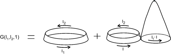
Figure 3.1: Illustration of a one step propagator with a “baby universe”.

This new, or “dressed”, one step propagator satisfies the same composition law as the bare transfer matrix (2.65), i.e.

$$G_{\lambda}(l_{1},l_{2};t_{1}+t_{2})=\sum_{l}G_{\lambda}(l_{1},l;t_{1})G_{\lambda}(l,l_{2};t_{2}).$$ (3.2)

Particularly this implies that the dressed one step propagator can still be used as a transfer matrix despite the fact that the disc function contains an infinite sum over time steps

$$G_{\lambda}(l_{1},l_{2};t)=\sum_{l}G_{\lambda}(l_{1},l;1)\;G_{\lambda}(l,l_{2};t\!-\!1).$$ (3.3)

Performing a (discrete) Laplace transformation of eq. (3.3) leads to

$${G(x,y;g;t)=}\leavevmode\nobreak\ \leavevmode\nobreak\ \leavevmode\nobreak\ \leavevmode\nobreak\ \leavevmode\nobreak\ \leavevmode\nobreak\ \leavevmode\nobreak\ \leavevmode\nobreak\ \leavevmode\nobreak\ \leavevmode\nobreak\ \leavevmode\nobreak\ \leavevmode\nobreak\ \leavevmode\nobreak\ \leavevmode\nobreak\ \leavevmode\nobreak\ \leavevmode\nobreak\ \leavevmode\nobreak\ \leavevmode\nobreak\ \leavevmode\nobreak\ \leavevmode\nobreak\ \leavevmode\nobreak\ \leavevmode\nobreak\ \leavevmode\nobreak\ \leavevmode\nobreak\ \leavevmode\nobreak\ \leavevmode\nobreak\ \leavevmode\nobreak\ \leavevmode\nobreak\ \leavevmode\nobreak\ \leavevmode\nobreak\ \leavevmode\nobreak\ \leavevmode\nobreak\ \leavevmode\nobreak\ \leavevmode\nobreak\ \leavevmode\nobreak\ \leavevmode\nobreak\ \leavevmode\nobreak\ \leavevmode\nobreak\ \leavevmode\nobreak\ \leavevmode\nobreak\ \leavevmode\nobreak\ \leavevmode\nobreak\ \leavevmode\nobreak\ \leavevmode\nobreak\ \leavevmode\nobreak\ \leavevmode\nobreak\ \leavevmode\nobreak\ \leavevmode\nobreak\ \leavevmode\nobreak\ \leavevmode\nobreak\ \leavevmode\nobreak\ \leavevmode\nobreak\ \leavevmode\nobreak\ \leavevmode\nobreak\ \leavevmode\nobreak\ \leavevmode\nobreak\ \leavevmode\nobreak\ \leavevmode\nobreak\ \leavevmode\nobreak\ \leavevmode\nobreak\ \leavevmode\nobreak\ \leavevmode\nobreak\ \leavevmode\nobreak\ \leavevmode\nobreak\ \leavevmode\nobreak\ \leavevmode\nobreak\ \leavevmode\nobreak\ \leavevmode\nobreak\ \leavevmode\nobreak\ \leavevmode\nobreak\ \leavevmode\nobreak\ \leavevmode\nobreak\ \leavevmode\nobreak\ \leavevmode\nobreak\ \leavevmode\nobreak\ \leavevmode\nobreak\ \leavevmode\nobreak\$$

$$\oint\frac{dz}{2\pi i\,z}\;\left[G_{\lambda}^{(b)}(x,z^{-1};1)\!+\!x\frac{\partial}{\partial x}\Bigl{(}w(x;g)G_{\lambda}^{(b)}(x,z^{-1};1)\Bigr{)}\right]G(z,y;g;t\!-\!1),$$

or, using the explicit form of the transfer matrix $G_{(b)}(x,z;g;1)$, formula (2.67),

$$G(x,y;g;t)=\Bigl{[}1+x\frac{\partial w(x,g)}{\partial x}+xw(x,g)\frac{\partial}{\partial x}\Bigr{]}\,\frac{gx}{1-gx}\,G\Bigl{(}\frac{g}{1\!-\!gx},y;g;t\!-\!1\Bigr{)}.$$ (3.5)

Note that this is not a closed equation, since so far neither the disc amplitude $w(x,g)$ nor $G(x,y;g;t)$ are known. Although this means that we cannot derive the discrete expressions, it will be shown by using scaling arguments that one can uniquely determine the continuum disc amplitude $W_{\Lambda}(X)$ and propagator $G_{\Lambda}(X,Y;T)$. As in the case for CDT without topology change we assume canonical scaling for both the boundaries and the cosmological constant,

$$g=\frac{1}{2}e^{-a^{2}\Lambda},\quad x=e^{-aX},\quad y=e^{-aY}.$$ (3.6)

In the following arguments no specific choice for the scaling of the time variable will be assumed as its scaling will be determined at a later stage. Interestingly, the composition law and the canonical scaling of the boundary lengths are enough to determine the scaling of the dressed propagator

$$G_{\lambda}(l_{1},l_{2},t)\buildrel a\rightarrow 0\over{\longrightarrow}a\,G_{\Lambda}(L_{1},L_{2};T).$$ (3.7)

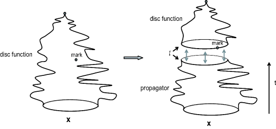
Figure 3.2: Decomposition of the marked CDT disc function in another CDT disc function and a propagator.

Changing the boundary conditions from fixed boundary length to fixed boundary cosmological constant amounts to taking a Laplace transformation and implementing the canonical scaling of the boundary cosmological constant $x=e^{-aX}$, leading to

$$G_{\lambda}(x,l_{2},t)\buildrel a\rightarrow 0\over{\longrightarrow}G_{\Lambda}(X,L_{2},T)$$ (3.8)

and

$$G_{\lambda}(x,y;t)\buildrel a\rightarrow 0\over{\longrightarrow}a^{-1}G_{\Lambda}(X,Y;T).$$ (3.9)

The scaling relation for the disc function is not as simple to obtain as the scaling for the propagator and we show that it actually depends on the scaling of time. Where for the propagator we use the composition law to derive its scaling relation we use the following exact combinatorial identity to determine the scaling relation for the disc function

$$g\ \frac{\partial w(x,g)}{\partial g}=\sum_{t}\sum_{l}G(x,l;g;t)\,l\,w(l,g),$$ (3.10)

or, after the usual Laplace transformation,

$$g\ \frac{\partial w(x,g)}{\partial g}=\sum_{t}\oint\frac{dz}{2\pi i\,z}\;G(x,z^{-1};g;t)\;\frac{\partial w(z,g)}{\partial z}.$$ (3.11)

These identities reflect the fact that if one introduces a mark anywhere in the bulk by taking a derivative with respect to $g$, the disc function can be decomposed into a propagator and another disc amplitude. The situation for the bare model is illustrated in fig. 3.2. In the figure on the right we have highlighted the points that have a distance $t$ to the entrance loop. Since the bare model does not allow for spatial topology change these points constitute one spatial universe with the topology of an $S^{1}$. In fig. 3.3 the situation is illustrated in the case where one does allow for topology change, in this case all points with equal distance $t$ from the entrance loop form a spatial section with the topology of several $S^{1}$’s and the mark is located on one of them.

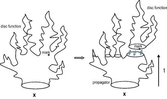
Figure 3.3: Decomposition of the disc function including spatial topology change.

Since our current objective is to find the scaling for the disc function we assume the following general scaling ansatz

$$w(x,g)=w_{ns}(x,g)+a^{\eta}W_{\Lambda}(X)+\mbox{less singular terms}.$$ (3.12)

In the case $\eta<0$ the first term is irrelevant in the continuum limit, it does not appear in the computation of any continuum quantities. However, if $\eta>0$ a term $w_{ns}$ will generically be present [60]. Additionally, the general ansatz for the scaling of the time variable reads as follows

$$T=a^{\varepsilon}t,\leavevmode\nobreak\ \leavevmode\nobreak\ \leavevmode\nobreak\ \leavevmode\nobreak\ \leavevmode\nobreak\ \varepsilon>0.$$ (3.13)

As shown in section (2.7.1) both space and time scale canonically in the bare model which corresponds to $\varepsilon=1$. Below we show that allowing the branching into baby universes to contribute to the continuum limit forces the scaling of time to be anomalous, creating an inherent asymmetry between the time- and space directions.

Inserting the scaling relations (3.12) and (2.55) into eq. (3.11) we obtain

$$\frac{\partial w_{ns}}{\partial g}-2a^{\eta-2}\frac{\partial W_{\Lambda}(X)}{\partial\Lambda}=$$

$$\hskip 17.07182pt\frac{1}{a^{\varepsilon}}\int\mbox{d}T\int dZ\;G_{\Lambda}(X,-Z;T)\bigg{[}\frac{\partial w_{ns}}{\partial z}-a^{\eta-1}\frac{1}{z_{c}}\frac{\partial W_{\Lambda}(Z)}{\partial Z}\bigg{]},$$ (3.14)

where $(x,g)=(x_{c},g_{c})$ in the non-singular part.

From eq. (3.14) and the requirement $\epsilon>0$ it follows that the only consistent choices for $\eta$ are

• ${\eta<\ }$0

  As can be seen from (3.12), this range of values corresponds to the situation where the non scaling part of the disc function is irrelevant and the physics is completely independent of the cutoff,

  $$a^{\eta-2}\frac{\partial W_{\Lambda}(X)}{\partial\Lambda}=\frac{a^{\eta-1}}{2a^{\varepsilon}}\int\mbox{d}T\int dZ\;G_{\Lambda}(X,-Z;T)\;\frac{1}{z_{c}}\frac{\partial W_{\Lambda}(Z)}{\partial Z}.$$ (3.15)

  The continuum limit can be taken for any $\eta<0$ since (3.15) does not depend on its explicit value. The value of $\varepsilon$ on the other hand is fixed and one needs to have $\varepsilon=1$ for the continuum limit to exist. Summarizing, if the scaling of the disc function is such that non scaling contributions are negligible in the continuum limit, the time variable automatically scales canonically. Obviously the bare CDT model falls in this class of scalings since it has $\eta=-1$ and $\varepsilon=1$.

• 1${\ <\eta<\ }$2.

  For this class of scalings for the disc function formula (3.14) splits into two equations

  $$-a^{\eta-2}\frac{\partial W_{\Lambda}(X)}{\partial\Lambda}=\frac{1}{2a^{\varepsilon}}\,\frac{\partial w_{ns}}{\partial z}\bigg{|}_{z=x_{c}}\;\int\mbox{d}T\int dZ\;G_{\Lambda}(X,-Z;T),$$ (3.16)

  and

  $$\frac{\partial w_{ns}}{\partial g}\bigg{|}_{g=g_{c}}=-\frac{a^{\eta-1}}{a^{\varepsilon}}\int\mbox{d}T\int dZ\;G_{\Lambda}(X,-Z;T)\;\frac{1}{z_{c}}\frac{\partial W_{\Lambda}(Z)}{\partial Z}.$$ (3.17)

  From (3.16) it follows that $a^{\eta-2}=\frac{1}{a^{\varepsilon}}$ and from (3.17) one sees that $\frac{a^{\eta-1}}{a^{\varepsilon}}=1$. Combining these requirements we are led to the conclusion that $\varepsilon=1/2$ and $\eta=3/2$, which are precisely the values found in Euclidean $2d$ gravity. Let us further remark that eq. (3.16) in this case becomes

  $$-\frac{\partial W_{\Lambda}(X)}{\partial\Lambda}=\mbox{const.}\;G_{\Lambda}(X,L_{2}=0).$$ (3.18)

  If one rescales the couplings it is possible in general to absorb the constant originating from the non universal terms. This implies that the continuum dynamics of the theory strongly depends on the fact that there are non universal terms surviving the continuum limit but their precise value does not play a pertinent role. It should be noted that (3.16) expresses a different relation between the disc function and the propagator than was used for the bare model, it differs from (2.61) by a derivative with respect to the cosmological constant. Finally, inserting $\varepsilon=1/2$ and $\eta=3/2$ into eq. (3.17) yields

  $$\int\mbox{d}T\int dZ\;G_{\Lambda}(X,-Z;T)\;\frac{\partial W_{\Lambda}(Z)}{\partial Z}=\mbox{const},$$ (3.19)

  where as in (3.18) the constant originates from the non scaling terms of the disc function and its value does not play a significant role in the continuum theory.

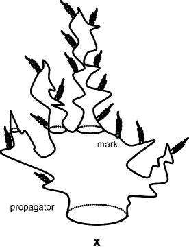
Figure 3.4: At every point in the quantum geometry there is an infinitesimal baby universe.

The relation (3.18) possesses a remarkable interpretation in terms of baby universes. Basically it states that near any mark in the bulk of the continuum Hartle Hawking wave function there is a baby universe at the scale of the cutoff. Since the location of the mark is arbitrary it implies that near every point there is a baby universe at the cutoff scale which is illustrated in fig. 3.4. This does not mean however that all baby universes are of negligible size. An additional indication that cutoff size geometries play an important role in the dynamics comes from the Laplace transform of (3.19)

$$\int\mbox{d}T\int dL\;G_{\Lambda}(L,L^{\prime};T)\;L^{\prime}\;W_{\Lambda}(L^{\prime})=\mbox{const}.\times\leavevmode\nobreak\ \delta(L),$$ (3.20)

which shows that the distribution of geometries is such that it is strongly peaked around universes that have minimal boundary length. In the following we show that these microscopic artifacts are an important feature of $2d$ Euclidean quantum gravity since the CDT model with baby universes exactly reproduces the continuum equations of the Euclidean model in the scaling limit. Furthermore, to make contact with the Euclidean theory, (3.18) is used in an essential way.

Having derived the scaling relations we can now analyze the scaling limit of (3.5) and find an equation for the dynamics of the propagator. In order for the equation to have a scaling limit at all, $x_{c},\,g_{c}$ and $w_{ns}(x_{c},g_{c})$ must satisfy two relations which can be determined straightforwardly from (3.5). The remaining continuum equation reads

$$a^{\varepsilon}\frac{\partial}{\partial T}\,G_{\Lambda}(X,Y;T) = -a\,\frac{\partial}{\partial X}\Bigl{[}(X^{2}-\Lambda)G_{\Lambda}(X,Y;T)\Bigr{]}$$ (3.21)

$$-a^{\eta-1}\frac{\partial}{\partial X}\Bigl{[}W_{\Lambda}(X)G_{\Lambda}(X,Y;T)\Bigr{]}.$$

The first term on the right-hand side of eq. (3.21) is precisely the one we have already encountered in the bare model, while the second term is due to the creation of baby universes. In case where $\eta\leq 1$ the first term in (3.21) is subdominant and the scaling will not be compatible with baby universes in the continuum limit. So from (3.21) it can be seen that for $\eta\leq 1$ we need to have that $\varepsilon=1$ leaving us with the continuum differential equation for the propagator of the bare model

$$\frac{\partial}{\partial T}\,G_{\Lambda}(X,Y;T)=-\frac{\partial}{\partial X}\Bigl{[}(X^{2}-\Lambda)G_{\Lambda}(X,Y;T)\Bigr{]},$$ (3.22)

where we remind the reader that this differential equation can naturally be interpreted as a Wick rotated Schrödinger equation of a single string propagating with respect to its own time on world sheet,

$$\frac{\partial}{\partial T}\,G_{\Lambda}(X,Y;T)=\hat{H}_{X}G_{\Lambda}(X,Y;T).$$ (3.23)

From the Laplace transform of this equation one sees that $\hat{H}$ is a simple Hamiltonian containing a kinetic term, a potential induced by the cosmological constant and no interaction terms,

$$\hat{H}^{\scriptscriptstyle marked}_{L}=-L\frac{\partial^{2}}{\partial L^{2}}+\Lambda\>L.$$ (3.24)

For the second scaling however, where $1<\eta<2$, the last term on the right-hand side of (3.21) will always dominate over the first term. Consequently, the first term does not survive the continuum limit leaving one with an equation without a Hamiltonian containing a kinetic term. So for this scaling the dynamics of the world sheet is governed purely by the interactions of splitting strings. Equivalently, we can say that once we allow for the creation of baby universes, this process will completely dominate the continuum limit. As we have seen from (3.16) and (3.17), $(\eta,\varepsilon)=(3/2,1/2)$ is the only consistent scaling that allows for baby universes. Inserting this scaling in (3.21) we obtain the following continuum equation

$$\frac{\partial}{\partial T}\,G_{\Lambda}(X,Y;T)=-\frac{\partial}{\partial X}\Bigl{[}W_{\Lambda}(X)G_{\Lambda}(X,Y;T)\Bigr{]},$$ (3.25)

which, combined with eq. (3.18), determines the continuum disc amplitude $W_{\Lambda}(X)$. Integrating (3.25) with respect to $T$ and using that $G_{\Lambda}(L_{1},L_{2};T\!=\!0)=\delta(L_{1}\!-\!L_{2})$, i.e.

$$G_{\Lambda}(X,L_{2}\!=\!0;T\!=\!0)=1,$$ (3.26)

we obtain

$$-1=\frac{\partial}{\partial X}\bigg{[}W_{\Lambda}(X)\frac{\partial}{\partial\Lambda}W_{\Lambda}(X)\bigg{]}.$$ (3.27)

From dimensional analysis one can easily see that $W_{\Lambda}^{2}(X)=X^{3}F(\sqrt{\Lambda}/X)$. This implies that the solution of the disc function reads as follows

$$W_{\Lambda}(X)=\sqrt{-2\Lambda X+b^{2}X^{3}+c^{2}\Lambda^{3/2}}.$$ (3.28)

However, not all values for $b$ and $c$ are physically acceptable. The inverse Laplace transform of (3.28), $W_{\Lambda}(L)$, should be bounded for all $L>0$. This constraint gives the following expression for the disc function

$$W_{\Lambda}(X)=b\Big{(}X-\frac{\sqrt{2}}{b\,\sqrt{3}}\,\sqrt{\Lambda}\Big{)}\sqrt{X+\frac{2\sqrt{2}}{b\,\sqrt{3}}\sqrt{\Lambda}},$$ (3.29)

where the constant $b$ is a constant that reflects specific details of the discrete statistical model, as described by equation (3.18). We discussed above that this constant does not have an obvious physical significance since it can be absorbed into the cosmological constant. Absorbing the irrelevant constant $b$ one obtains the disc function $W^{(eu)}_{\Lambda}(X)$ of 2d Euclidean quantum gravity,

$$W_{\Lambda}(X)=(X-\frac{1}{2}\sqrt{\Lambda})\sqrt{X+\sqrt{\Lambda}}.$$ (3.30)

Note that the defining equation for the disc function (3.25), can alternatively be derived by several methods within 2d Euclidean quantum gravity [37, 60, 61]. In those computations it is clear that $T$ can be interpreted as the geodesic distance between the initial and final loop.

For a more detailed account on baby universes in two dimensional Euclidean quantum gravity the reader is referred to [62].

3.2 Introducing the new coupling constant

In this section we present a model which can be viewed as a hybrid between Euclidean and causal quantum gravity. Recall that the pure CDT model possesses a Hamiltonian that governs the dynamics of an individual string, but that there is no interaction term in the dynamical equation to allow for spatial topology change (3.22). In the case of the Euclidean theory the opposite is true, the equation governing the dynamics of the propagator only contains an interaction term and no kinetic or potential terms for an individual string (3.25). In the previous section it was shown that both theories can be obtained by two different scaling limits of one unifying statistical model based on CDT (3.1). The current objective is to show that there is a natural adaptation of this unifying model such that its scaling limit acquires single string dynamics while at the same time allowing interactions in the form of spatial topology change. The essential ingredient in accomplishing this is to introduce a new coupling in the statistical model (3.1) whose scaling is such that both the interaction term and the dynamical term in (3.1) contribute in the continuum limit.

Figure 3.5: A representation of the global aspects of a trouser geometry with modular parameters ($\tau_{1},\tau_{2},\tau_{3}$).

Before discussing the construction of the model we examine some aspects of geometries with spatial topology change. The simplest example of a two dimensional geometry with spatial topology change is the so-called “trouser” geometry. A trouser geometry is a manifold with three boundary components with the topology of an $S^{1}$. In general the so-called legs of the trousers can have any length which can be parameterized by three modular parameters as illustrated in fig. 3.5 .

We are interested however in a more restricted subclass of trouser geometries which are of the form depicted in fig. 3.6. We demand that we have an initial boundary, where every point on this boundary has the same distance to the two final loops. This restriction means that on top of the length of the boundary components we need just two parameters to describe the global characteristics of the geometries, one describing the length of the trouser leg belonging to the initial boundary component and one that specifies the length of the trouser legs related to the final boundary components. since we required the final boundary components to have the same distance to the initial boundary.

Now we ask ourselves the question, what is the contribution of such a geometry to the path integral? As described in chapter 2 the action for two dimensional gravity contains just a volume term proportional to the cosmological constant and a topological term coming from the two dimensional Einstein-Hilbert action and the Gibbons-Hawking-York boundary term,

$$S_{M}=\Lambda V_{M}+\tfrac{2\pi}{G_{N}}\chi(M),$$ (3.31)

where $\chi(M)=\left(2-2{\mathfrak{g}}-b\right)$ is the Euler characteristic of the manifold. The weight of an individual geometry in the path integral is therefore proportional to the exponential of the volume and the exponential of the number of handles and boundary components.

$$G_{G_{N},\Lambda}(L_{1},L_{2},T)=\sum_{topol.}g^{2{\mathfrak{g}}}_{S}\int_{M}D[g_{\mu\nu}]e^{i\Lambda V_{M}}.$$ (3.32)

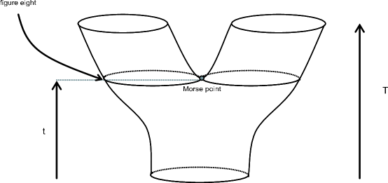
Figure 3.6: A representation of the global geometry of a trouser geometry in causal dynamical triangulations

We see that geometries with the topology of a cylinder are not weighted by $g_{S}$, since the Euler characteristic of a cylinder is zero. The Euler characteristic of a trouser geometry is one however, since the trouser geometry has one more boundary component than the cylinder. Consequently the weight of the trouser geometry in the path integral is not only determined by the cosmological constant, but also by the coupling $g_{S}$. For the purposes of this thesis we are not particularly interested in computing amplitudes with the topology of a trouser, but we are interested in calculating propagators, i.e. amplitudes that have two macroscopic boundary components. If one shrinks one of the final boundary components of a trouser geometry to zero one obtains a geometry with two boundary components that we interpret as a “cylinder geometry with one baby universe”. Shrinking a boundary component does not alter the Euler characteristic, allowing us to conclude that a geometry with $n$ baby universes contributes to the path integral with a $g_{S}^{n}$ topological weight. Note that in the derivation of the disc amplitude of Euclidean dynamical triangulations of section (3.1) we did not associate a coupling constant to the baby universes. Subsequently, the formation of baby universe was not suppressed with the result that the continuum limit is dominated by cutoff scale baby universes. In section (3.3) we show that adding the coupling constant makes the term baby universes a bit misleading since the outgrowths have a certain finite size in the continuum limit and can be made arbitrarily big or small depending on the value of $g_{S}$.

3.2.1 Lorentzian aspects

The reasoning in the previous section was based on a picture where the metrics are Wick rotated from Lorentzian to Euclidean signature. Performing an inverse Wick rotation is not so easy however for geometries with baby universes, since these geometries do not admit Lorentzian metric everywhere. The reason for this comes from the fact that it is not possible to find a non vanishing vector field everywhere. It is however possible to find a vector field everywhere except for a finite number of points. For some values of the time parameter the universe develops a baby universe and the topology of a spatial universe splits up into two different components. Precisely at the moment of a split the spatial geometry has the topology of a figure eight and we see that the central point of the figure eight is a saddle point if one views the geometry as being embedded in $\mathbb{R}^{3}$. This point is called a Morse point in the mathematically oriented literature [57]. Contrary to a generic point on the manifold, such a Morse point does not possess a unique timelike vector field perpendicular to its spatial slice. In fact it has two future directed normal timelike vectors, showing that the neighborhood of such a point has an anomalous causal structure. More precisely, such a point has two future, and two past light cones which we refer to as a double light cone structure [57]. Consequently, if one universe splits in two, each of the resulting universes carries a light cone belonging to the Morse point as is illustrated in fig. 3.7. Conversely, the universe carries the two past light cones of the Morse point before the split.

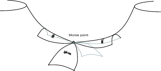
Figure 3.7: Illustration of the double light cone causal structure around a Morse point.

Because of the peculiar causal structure around the Morse points we are not quite sure whether the usual definition of the Wick rotation in CDT is also legitimate here. There are some indications that the Einstein Hilbert action develops complex valued singularities at these points [63]. Although the Wick rotation at these points presents one with an interesting conundrum, we confine ourselves to the Euclidean sector for the remainder of this thesis.

3.3 Dynamics to all orders in the coupling

In this section we discuss the explicit construction of the model with a coupling constant for the spatial topology changes and show that it can be solved to all orders in the coupling constant in a suitable continuum limit.

Our starting point is equation (3.1) with the addition of a coupling to the interaction term, where in section (3.2) we argued that the coupling can naturally be denoted as $g_{s}$,

$$G_{\lambda}(l_{1},l_{2};1)=G_{\lambda}^{(b)}(l_{1},l_{2};1)+2g_{s}\sum_{l=1}^{l_{1}-1}l_{1}w_{\lambda,g_{s}}(l_{1}\!-\!l)\,G_{\lambda}^{(b)}(l,l_{2};1).$$ (3.33)

After a discrete Laplace transform one obtains

$${G(x,y;g;t)=}\leavevmode\nobreak\ \leavevmode\nobreak\ \leavevmode\nobreak\ \leavevmode\nobreak\ \leavevmode\nobreak\ \leavevmode\nobreak\ \leavevmode\nobreak\ \leavevmode\nobreak\ \leavevmode\nobreak\ \leavevmode\nobreak\ \leavevmode\nobreak\ \leavevmode\nobreak\ \leavevmode\nobreak\ \leavevmode\nobreak\ \leavevmode\nobreak\ \leavevmode\nobreak\ \leavevmode\nobreak\ \leavevmode\nobreak\ \leavevmode\nobreak\ \leavevmode\nobreak\ \leavevmode\nobreak\ \leavevmode\nobreak\ \leavevmode\nobreak\ \leavevmode\nobreak\ \leavevmode\nobreak\ \leavevmode\nobreak\ \leavevmode\nobreak\ \leavevmode\nobreak\ \leavevmode\nobreak\ \leavevmode\nobreak\ \leavevmode\nobreak\ \leavevmode\nobreak\ \leavevmode\nobreak\ \leavevmode\nobreak\ \leavevmode\nobreak\ \leavevmode\nobreak\ \leavevmode\nobreak\ \leavevmode\nobreak\ \leavevmode\nobreak\ \leavevmode\nobreak\ \leavevmode\nobreak\ \leavevmode\nobreak\ \leavevmode\nobreak\ \leavevmode\nobreak\ \leavevmode\nobreak\ \leavevmode\nobreak\ \leavevmode\nobreak\ \leavevmode\nobreak\ \leavevmode\nobreak\ \leavevmode\nobreak\ \leavevmode\nobreak\ \leavevmode\nobreak\ \leavevmode\nobreak\ \leavevmode\nobreak\ \leavevmode\nobreak\ \leavevmode\nobreak\ \leavevmode\nobreak\ \leavevmode\nobreak\ \leavevmode\nobreak\ \leavevmode\nobreak\ \leavevmode\nobreak\ \leavevmode\nobreak\ \leavevmode\nobreak\ \leavevmode\nobreak\ \leavevmode\nobreak\ \leavevmode\nobreak\ \leavevmode\nobreak\ \leavevmode\nobreak\ \leavevmode\nobreak\ \leavevmode\nobreak\ \leavevmode\nobreak\ \leavevmode\nobreak\ \leavevmode\nobreak\ \leavevmode\nobreak\ \leavevmode\nobreak\ \leavevmode\nobreak\ \leavevmode\nobreak\$$

$$\oint\frac{dz}{2\pi i\,z}\;\left[G^{(b)}(x,z^{-1};g;1)\!+\!\leavevmode\nobreak\ 2g_{s}\leavevmode\nobreak\ x\frac{\partial}{\partial x}\Bigl{(}w_{g_{s}}(x;g)G^{(b)}(x,z^{-1};g;1)\Bigr{)}\right]G(z,y;g;t\!-\!1).$$

If the baby universes are to survive the continuum limit the coupling constant in a controlled manner we have to scale $g_{S}$ with the lattice cutoff $a$. To find the appropriate scaling for the coupling we implement the following ansatz

$$g_{s}=a^{\xi}g_{S}+\mbox{less singular terms.}$$ (3.35)

Using the explicit form of the transfer matrix $G_{\lambda}^{(b)}(x,z^{-1};1)$ and inserting the scaling relations (2.55), (3.35) into expression (LABEL:eq:Gxygtdressedcomposition) one is led to the following continuum equation,

$$a^{\varepsilon}\frac{\partial}{\partial T}\,G_{\Lambda}(X,Y;T) = -a\,\frac{\partial}{\partial X}\Bigl{[}(X^{2}-\Lambda)G_{\Lambda}(X,Y;T)\Bigr{]}$$ (3.36)

$$-2g_{S}\>a^{\eta+\xi-1}\frac{\partial}{\partial X}\Bigl{[}{W}_{\Lambda,g_{S}}(X)G_{\Lambda}(X,Y;T)\Bigr{]}.$$

If we demand that the first term on the right hand side of eq. (3.36) survives the continuum limit we need $\epsilon=1$ as in the bare CDT model. Contrary to (3.21) we have the additional freedom to scale the coupling constant $g_{S}$. This enables us to adjust the scaling so that also the second term survives the continuum limit yielding $\eta+\xi=2$. Inserting this relation in (3.36) we obtain the desired dynamical equation that contains both the dynamical term for propagation of single strings and a term governing string interactions,

$$\frac{\partial}{\partial T}G^{(1;0)}(X,Y,T)=-\frac{\partial}{\partial X}\left[\left((X^{2}-\Lambda)+2g_{S}{W}_{\Lambda,g_{S}}(X)\right)G^{(1;0)}(X,Y,T)\right].$$ (3.37)

We observe that this equation is of the same form as the equations for the CDT models without a coupling constant (2.69),

$$\frac{\partial}{\partial T}G^{(1;0)}(X,Y;T)=-\frac{\partial}{\partial X}\left[{\hat{W}}_{\Lambda,g_{S}}(X)G^{(1;0)}(X,Y;T)\right],$$ (3.38)

but with a different form of ${\hat{W}}(X)$,

$${\hat{W}}_{\Lambda,g_{S}}(X)=(X^{2}-\Lambda)\;+\;2g_{S}\>{W}_{\Lambda,g_{S}}(X).$$ (3.39)

Note that requiring both terms in (3.37) to survive the scaling limit does not fix the scaling uniquely. However, since we merely introduce a coupling constant to the baby universe model and did not introduce any new configurations in the path integral, the disc function should still satisfy (3.10). As before we can use this relation to further constrain the scaling. The dynamics of our new model requires $\varepsilon=1$, so we are led to the conclusion that the model falls into the first of the two scaling classes defined in section (3.1) implying $\eta<0$. Consequently, the relation between the continuum disc function and the continuum propagator is the same as for the bare CDT model,

$$\frac{\partial{W}_{\Lambda,g_{S}}(X)}{\partial\Lambda}=\int dT\int dZG^{(1;0)}(X,-Z;T)\frac{\partial{W}_{\Lambda,g_{S}}}{\partial Z}.$$ (3.40)

It seems that we are still left with a predicament since we are unable to specify the exact scaling for the disc function. In fact it is only an illusory problem, since the disc function only appears in the dynamical equations in combination with the coupling constant as $g_{S}{W}$. Therefore, we in principle only need to determine the scaling of this combination which means that the relevant part of the scaling is already determined by the dynamical equation itself. In the model we consider however, the scaling is completely fixed by requiring the disc function to reduce to the disc function of the bare CDT model for zero $g_{S}$, implying

$$w_{\lambda,g_{s}}(x)=a^{-1}{W}_{\Lambda,g_{S}}(X),\quad g_{s}=a^{3}g_{S}.$$ (3.41)

In the remainder of this section (3.40) and (3.37) are used to derive a differential equation for ${\hat{W}}_{\Lambda,g_{S}}(X)$. The equation will be rather implicit however, since the equation does not only depend on ${\hat{W}}_{\Lambda,g_{S}}(X)$, but it also depends explicitly on the solution of the equation ${\hat{W}}_{\Lambda,g_{S}}(X)=0$. Remarkably, one is able to solve the equation uniquely provided the disc functions ${W}_{\Lambda,g_{S}}(L)$ satisfy the natural physical requirement that they fall of at infinity. As a first step we solve the dynamical equation (3.37) to obtain the propagator in terms of ${\hat{W}}_{\Lambda,g_{S}}(X)$,

$$G^{(1;0)}(X,Y,T)=\frac{{\hat{W}}_{\Lambda,g_{S}}({\bar{X}}(T))}{{\hat{W}}_{\Lambda,g_{S}}(X)}\frac{1}{{\bar{X}}(T)+Y}.$$ (3.42)

Inserting this into the consistency condition (3.40) and performing the integration over $Z$ we obtain

$$\frac{\partial{W}_{\Lambda,g_{S}}(X)}{\partial\Lambda}=-\int dT\frac{{\hat{W}}_{\Lambda,g_{S}}({\bar{X}}(T))}{{\hat{W}}_{\Lambda,g_{S}}(X)}\frac{\partial{W}_{\Lambda,g_{S}}}{\partial{\bar{X}}(T)}.$$ (3.43)

To evaluate the integral we conveniently use the characteristic equation and convert the integral over time into an integral over ${\bar{X}}$,

$$\frac{d{\bar{X}}}{dT}=-{\hat{W}}_{\Lambda,g_{S}}({\bar{X}}(T)).$$ (3.44)

Applying the characteristic equation to (3.43) we obtain

$$\frac{\partial{W}_{\Lambda,g_{S}}(X)}{\partial\Lambda}=\frac{1}{{\hat{W}}_{\Lambda,g_{S}}(X)}\int\limits^{{\bar{X}}_{\infty}}_{X}d{\bar{X}}\frac{\partial{W}_{\Lambda,g_{S}}}{\partial{\bar{X}}},$$ (3.45)

where one can easily evaluate the integral since the integrand is a total derivative,

$$\frac{\partial{W}_{\Lambda,g_{S}}(X)}{\partial\Lambda}=\frac{{W}_{\Lambda,g_{S}}(X)-{W}_{\Lambda,g_{S}}({\bar{X}}_{\infty})}{{\hat{W}}_{\Lambda,g_{S}}(X)}.$$ (3.46)

This equation can be rewritten as an equation for ${\hat{W}}_{\Lambda,g_{S}}(X)$ by reexpressing the disc functions as

$${W}_{\Lambda,g_{S}}(X)=-\frac{{\hat{W}}_{\Lambda,g_{S}}(X)-(X^{2}-\Lambda)}{2g_{S}},$$ (3.47)

giving

$$\frac{\partial{\hat{W}}_{\Lambda,g_{S}}(X)}{\partial\Lambda}=\frac{{\bar{X}}_{\infty}^{2}-X^{2}}{{\hat{W}}_{\Lambda,g_{S}}(X)},$$ (3.48)

or equivalently,

$$\frac{\partial{\hat{W}}_{\Lambda,g_{S}}(X)^{2}}{\partial\Lambda}=2({\bar{X}}_{\infty}^{2}-X^{2}).$$ (3.49)

This is the defining equation for ${\hat{W}}_{\Lambda,g_{S}}(X)$ that we intended to derive. The simple form of the equation is deceptive as ${\bar{X}}_{\infty}$ is in fact a completely unknown function of $g_{S}$ and $\Lambda$, the only thing we know is that it is defined as the solution of ${\hat{W}}_{\Lambda,g_{S}}(X)=0$. Another unknown arises when we try to solve (3.49) by integrating both sides with respect to $\Lambda$, the integration “constant”, $C(g_{S},X)$, can in principle be a general function of $g_{S}$ and $X$. So we conclude that (3.49) only determines ${\hat{W}}_{\Lambda,g_{S}}(X)$ up to two functions. Explicitly, the integral of (3.49) can be written as follows,

$${\hat{W}}_{\Lambda,g_{S}}(X)^{2}=\Lambda^{2}f\left(\textstyle{\frac{g_{S}}{\sqrt{\Lambda}^{3}}}\right)-2X^{2}\Lambda+X^{4}h\left(\textstyle{\frac{g_{S}}{X^{3}}}\right),$$ (3.50)

where we have used dimensional analysis to parameterize the integration constant and the integral of ${\bar{X}}_{\infty}$ by two dimensionless functions,

$$\Lambda^{2}f\left(\textstyle{\frac{g_{S}}{\sqrt{\Lambda}^{3}}}\right)=2\int^{\Lambda}d\Lambda^{\prime}{\bar{X}}_{\infty}\left(\textstyle{g_{S},\sqrt{\Lambda^{\prime}}^{3}}\right),\quad C(g_{S},X)=X^{4}h\left(\textstyle{\frac{g_{S}}{X^{3}}}\right).$$ (3.51)

Below we use the following series expansions

$$f\left(\textstyle{\frac{g_{S}}{\sqrt{\Lambda}^{3}}}\right)=\sum\limits_{n=0}^{\infty}f_{n}\left(\textstyle{\frac{g_{S}}{\sqrt{\Lambda}^{3}}}\right)^{n},\quad h\left(\textstyle{\frac{g_{S}}{X^{3}}}\right)=\sum\limits_{n=0}^{\infty}h_{n}\left(\textstyle{\frac{g_{S}}{X^{3}}}\right)^{n}.$$ (3.52)

We show that the lowest order coefficients of the expansions are determined by requiring consistency with the bare CDT model. Amazingly, all higher order coefficients are uniquely determined by demanding that the inverse Laplace transform of the disc function ${W}(X)$ falls of at infinity at arbitrary order in the $g_{S}$ expansion. From the definition of ${\hat{W}}(X)$ in the pure model (2.70) one readily sees that to lowest order in $g_{S}$ we need to have

$${\hat{W}}_{\Lambda,g_{S}}(X)^{2}=X^{4}-2X^{2}\Lambda+\Lambda^{2}+{\cal O}(g_{S}),$$ (3.53)

which implies $h_{0}=1,f_{0}=1$ when comparing to (3.50). Using this result we write the disc function as follows,

$${W}_{\Lambda,g_{S}}(X)=\frac{-(X^{2}-\Lambda)+(X^{2}-\Lambda)\sqrt{1+\frac{\sum\limits_{n=1}^{\infty}g_{S}^{n}\left(h_{n}X^{4-3n}+f_{n}\sqrt{\Lambda}^{4-3n}\right)}{(X^{2}-\Lambda)^{2}}}}{2g_{S}}.$$ (3.54)

If we expand this expression to lowest order in $g_{S}$ we obtain

$${W}_{\Lambda,g_{S}}(X)=\frac{1}{4}\frac{h_{1}X+f_{1}\sqrt{\Lambda}}{X^{2}-\Lambda}+{\cal O}(g_{S}).$$ (3.55)

By equating this result to the marked disc function of the bare model

$${W}_{\Lambda,0}(X)=\frac{1}{X+\sqrt{\Lambda}},$$ (3.56)

we conclude that $h_{1}=4,f_{1}=-4$. To obtain the higher order coefficients we proceed by analyzing the $g_{S}$ expansion of the disc function order by order. The first order correction to the disc function is obtained by inserting $h_{1}=4,f_{1}=-4$ into (3.54) and expanding to first order in the coupling,

$${W}_{\Lambda,g_{S}}(X)=\textstyle{\frac{1}{X+\sqrt{\Lambda}}+g_{S}\left(-\frac{1}{(X^{2}-\Lambda)(X+\sqrt{\Lambda})^{2}}+\frac{h_{2}(4X)^{-2}+f_{2}(4\sqrt{\Lambda})^{-2}}{X^{2}-\Lambda}\right)+{\cal O}(g_{S}^{2})}.$$ (3.57)

After an inverse Laplace transform we obtain

$$\sqrt{\Lambda}^{3}{W}_{\Lambda,1}(L)=\frac{1}{8}e^{L\sqrt{\Lambda}}(f_{2}+h_{2}-1)-\frac{h_{2}L}{4}+\frac{1}{8}e^{-L\sqrt{\Lambda}}\left(2\Lambda L^{2}+2\sqrt{\Lambda}L-f_{2}-h_{2}+1\right),$$ (3.58)

where we have introduced the following notation

$${W}_{\Lambda,g_{S}}(X)=\sum\limits_{n=0}^{\infty}{W}_{\Lambda,n}(X)g_{S}^{n}.$$ (3.59)

Demanding the disc function to fall of at infinity implies that the terms proportional to $L$ and $e^{L\sqrt{\Lambda}}$ must vanish, leading to $h_{2}=0,f_{2}=1$. So the result for the disc function at first order in the coupling reads as follows,

$${W}_{\Lambda,1}(L)=\frac{e^{-L\sqrt{\Lambda}}L\left(\sqrt{\Lambda}L+1\right)}{4\Lambda},$$ (3.60)

which can be confirmed by explicitly computing the “Feynman diagram” where the spatial universe is allowed to split once. Obtaining the higher order coefficients is a bit messy, but the iterative procedure to compute them is completely analogous to the calculation for $h_{2}$ and $f_{2}$. At each order of the $g_{S}$ expansion the disc function has the same form as (3.60). Every ${W}_{\Lambda,n}(L)$ contains three terms, a polynomial term in $L$, a term proportional to $e^{\sqrt{\Lambda}L}$ and a term proportional to $e^{-\sqrt{\Lambda}L}$. Demanding the disc function to be bounded at infinity implies that the polynomial and ${\cal O}(e^{\sqrt{\Lambda}L})$ terms should vanish. If one additionally uses the known results for $h_{n-1}$ and $f_{n-1}$ one obtains the $h_{n}$ and $f_{n}$ coefficients uniquely. It turns out that boundedness of the disc function is such a stringent constraint that we need $h_{n}=0$ for all $n\geq 2$. Inserting the nonzero coefficients of $h\left(\textstyle{\frac{g_{S}}{X^{3}}}\right)$ into (3.50) we obtain

$${\hat{W}}_{\Lambda,g_{S}}(X)^{2}=X^{4}-2X^{2}\Lambda+4g_{S}X+F(g_{S},\Lambda),$$ (3.61)

where

$$F(g_{S},\Lambda)=\Lambda^{2}f(q),\quad q=\textstyle{\frac{g_{S}}{\sqrt{\Lambda}^{3}}}.$$ (3.62)

As noted above, demanding the disc function to be bounded at infinity also fixes all $f_{n}$. Contrary to the $h_{n}$ coefficients however, the $f_{n}$ coefficients are rather nontrivial but can be computed by the algorithm sketched above. Employing a symbolic computer program such as Mathematica one can readily compute the first coefficients ($\sim 20$). Making use of Sloan’s database of integer sequences it is possible to find a closed analytical expression for the coefficients $f_{n}$ in terms of Euler gamma functions,

$$f_{0}=1,\quad f_{n}=\frac{\Gamma(\frac{3}{2}n-2)}{\Gamma(\frac{1}{2}n+1)\Gamma(n)},\quad n\geq 1.$$ (3.63)

Given these coefficients we can sum the Taylor expansion and obtain the full non perturbative result for $f\left(q\right)$

$$f(q)={\textstyle\frac{2}{3}+\frac{1}{3}}\,_{2}F_{1}\left({\textstyle-\frac{1}{3},-\frac{2}{3};\frac{1}{2};\frac{2}{3\sqrt{3}}}q\right)-{\textstyle 4_{2}F_{1}}\left({\textstyle-\frac{1}{6},\frac{1}{6};\frac{3}{2};\frac{2}{3\sqrt{3}}}q\right).$$ (3.64)

This means that we have solved our model and we can present the disc function with a non perturbative sum over spatial topologies,

$${W}_{\Lambda,g_{S}}(X)=\frac{-(X^{2}-\Lambda)+\sqrt{X^{4}-2X^{2}\Lambda+4q\sqrt{\Lambda}^{3}X+\Lambda^{2}f\left(q\right)}}{2g_{S}}.$$ (3.65)

3.4 Relation to random trees

In this section we give an alternative derivation of the disc function dressed with spatial topology changes (3.65) to show robustness of the result and to give more insight into the details of the quantum geometry. Particularly, the derivation we present below highlights the random tree structure of the configurations. To make the connection as clear as possible we start by deriving the one point function for a random tree model. Sometimes this one point function for random trees is referred to as a partition function for rooted branched polymers. The random tree model we consider is a statistical model consisting of edges that are weighted with a fugacity $z$ and three-valent vertices with a coupling constant $\lambda$. A convenient way to view the partition function $w(z,g)$ is that it is the generating function for the number of random trees,

$$w(z,\lambda)=z\sum\limits_{m=0}^{\infty}w_{2m}\left(\lambda z^{2}\right)^{m},$$ (3.66)

where we use the fact that every vertex except the initial, or marked, vertex is accompanied by two edges. An easy way to evaluate the partition function $w(z,\lambda)$ is to notice that it should solve the following equation

$$w(z,\lambda)=z+\lambda zw(z,\lambda)^{2}.$$ (3.67)

Figure 3.8: Pictorial representation of the iterative equation for the one-point function $w(\lambda,z)$ for branched polymers.

The interpretation of this equation is illustrated in fig. 3.8. Equation (3.67) has two solutions but only one solution is compatible with the initial condition that there is only one tree with one edge, i.e. $w_{2m}=1$. This solution is given by

$$w(z,\lambda)=\frac{1-\sqrt{1-4\lambda z^{2}}}{2\lambda z},$$ (3.68)

which has the following series expansion,

$$w(z,\lambda)=z\sum\limits_{m=0}^{\infty}\frac{(2m)!}{m!(m+1)!}\left(\lambda z^{2}\right)^{m}.$$ (3.69)

So we see that the number of random trees with $m$ edges, $w_{2m}$, is given by the $m^{th}$ Catalan number. This random tree model can be regarded as a simple model possessing some features of $\phi^{3}$ theory. Indeed it is possible to formulate scalar $\phi^{3}$ theory in $\mathbb{R}^{d}$ as a sum over connected diagrams in the same way as the random tree model. One merely needs to replace the fugacity of the edges $z$ by the standard scalar propagators. Here we view the random trees not as a model for particles interacting in an ambient space, but as a simple model for a theory of “interacting universes” in two dimensional quantum gravity. The idea is similar to the basic idea behind string theory, we “blow up” the Feynman diagrams by replacing the propagators of an interacting field theory by the propagators of a string theory as is illustrated in fig. 3.9. In our case this means that we replace the rather trivial propagators of the branched polymer model $z$ by propagators that we computed from CDT (2.73). We remind the reader that the resulting model can either be viewed as a toy model for quantum gravity with topology change or as a string theory without a target space. To make the analogy as close as possible we write the equation for the generating function of the branched polymer as follows,

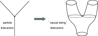
Figure 3.9: Illustration of spatial topology change as a string like generalization of a particle interaction.

$$w(z,\lambda)=w_{0}(z)+\lambda G_{0}(z)w(z,\lambda)^{2},$$ (3.70)

where $w_{0}(z)$ and $G_{0}(z)$ denote the one point function and the two point function respectively, to zeroth order in the coupling $\lambda$. From (3.67) we observe that the expressions for these objects coincide $w_{0}(z)=G_{0}(z)=z$. This is an understandable coincidence, since the branched polymer is a very simple model. The equation analogous to (3.70) for our model of interacting spatial universes based on CDT is

$${W}_{\Lambda,g_{S}}(L)={W}_{\Lambda,0}(L)+g_{S}\int dTdL_{1}dL_{2}G^{(1,1)}_{\Lambda,0}(L,L_{1}+L_{2};T){W}_{\Lambda,g_{S}}(L_{1}){W}_{\Lambda,g_{S}}(L_{2}).$$ (3.71)

This is the defining equation for the disc function ${W}(L)$. It is similar to the way equation (3.70) defines the one point function of the branched polymers $w(z,\lambda)$, since the disc function is the CDT analogue of the branched polymer one point function $w(z,\lambda)$. Instead of solving (3.71) we work with its Laplace transformed analogue,

$${W}_{\Lambda,g_{S}}(X)={W}_{\Lambda,0}(X)+g_{S}\int dZ_{1}dZ_{2}G^{(1,1}_{\Lambda,0}(X;-Z_{1},-Z_{2}){W}_{\Lambda,g_{S}}(Z_{1}){W}_{\Lambda,g_{S}}(Z_{2}),$$ (3.72)

where the propagator is given by

$$G^{(1,1)}(X;Y_{1},Y_{2};T)=\frac{{\hat{W}}_{\Lambda,0}({\bar{X}})}{{\hat{W}}_{\Lambda,0}(X)}\left[\frac{1}{({\bar{X}}+Y_{1})^{2}({\bar{X}}+Y_{2})}+\frac{1}{({\bar{X}}+Y_{1})({\bar{X}}+Y_{2})^{2}}\right].$$ (3.73)

Performing the integrations over $Z_{1}$ and $Z_{2}$ in (3.72) gives

$${W}_{\Lambda,g_{S}}(X)={W}_{\Lambda,0}(X)+g_{S}\int dT\frac{{\hat{W}}_{\Lambda,0}({\bar{X}}(T))}{{\hat{W}}_{\Lambda,0}(X)}\frac{\partial{W}_{\Lambda,g_{S}}({\bar{X}})^{2}}{\partial{\bar{X}}}.$$ (3.74)

As in (3.43) it is convenient to use the characteristic equation to convert the integral over $T$ into an integral over ${\bar{X}}(X,T)$,

$${W}_{\Lambda,g_{S}}(X)={W}_{\Lambda,0}(X)+\frac{g_{S}}{{\hat{W}}_{\Lambda,0}(X)}\int\limits_{X}^{{\bar{X}}_{\infty}}d{\bar{X}}\frac{\partial{W}_{\Lambda,g_{S}}({\bar{X}})^{2}}{\partial{\bar{X}}}.$$ (3.75)

Seeing that the integrand is a total derivative one easily obtains

$${W}_{\Lambda,g_{S}}(X)={W}_{\Lambda,0}(X)+g_{S}\frac{{W}_{\Lambda,g_{S}}({\bar{X}}_{\infty})^{2}-{W}_{\Lambda,g_{S}}(X)^{2}}{{\hat{W}}_{\Lambda,0}(X)}.$$ (3.76)

Since this is a second order polynomial equation for ${W}(X)$ it is readily solved and we obtain,

$${W}_{\Lambda,g_{S}}(X)=\frac{-{\hat{W}}_{\Lambda,0}(X)+{\hat{W}}_{\Lambda,g_{S}}(X)}{2g_{S}},$$ (3.77)

where

$${\hat{W}}_{\Lambda,g_{S}}(X)=\sqrt{{\hat{W}}_{\Lambda,0}(X)^{2}+4g_{S}\left({\hat{W}}_{\Lambda,0}(X){W}_{\Lambda,0}(X)+g_{S}{W}_{\Lambda,g_{S}}({\bar{X}}_{\infty})^{2}\,\right)}.$$ (3.78)

Note that this equation was derived independently of the particular form of ${W}_{\Lambda,0}(X)$ and ${\hat{W}}_{\Lambda,0}(X)$. Currently, however we are interested in an interacting model based on CDT. So we require the disc function and the propagator to reduce to the results obtained in the bare CDT theory,

$${W}_{\Lambda,0}(X)=\frac{1}{X+\sqrt{\Lambda}},\quad{\hat{W}}_{\Lambda,0}(X)=X^{2}-\Lambda,\quad{\bar{X}}_{\infty}=\sqrt{\Lambda}.$$ (3.79)

Inserting into (3.78) gives,

$${\hat{W}}_{\Lambda,g_{S}}(X)^{2}=(X^{2}-\Lambda)^{2}+4g_{S}\left((X-\sqrt{\Lambda})+g_{S}{W}_{\Lambda,g_{S}}(\sqrt{\Lambda})^{2}\,\right),$$ (3.80)

which can be conveniently written as

$${\hat{W}}_{\Lambda,g_{S}}(X)^{2}=X^{4}-2X^{2}\Lambda+4g_{S}X+F(g_{S},\Lambda),$$ (3.81)

where

$$F(g_{S},\Lambda)=\Lambda^{2}-4g_{S}\sqrt{\Lambda}+4g_{S}^{2}{W}_{\Lambda,g_{S}}(\sqrt{\Lambda})^{2}.$$ (3.82)

Given (3.81) and (3.39) we can obtain the following result for the disc function,

$${W}_{\Lambda,g_{S}}(X)=\frac{-(X^{2}-\Lambda)+\sqrt{X^{4}-2X^{2}\Lambda+4g_{S}X+F(g_{S},\Lambda)}}{2g_{S}},$$ (3.83)

which is exactly of the same form as derived in the previous section (3.3) but so far we have not yet determined the precise form of $F(g_{S},\Lambda)$. To abbreviate the notation, we can convert the equation to dimensionless units by dividing all dimensional quantities by appropriate powers of the cosmological constant

$$x=\tfrac{X}{\sqrt{\Lambda}},\leavevmode\nobreak\ \leavevmode\nobreak\ Y=\tfrac{Y}{\sqrt{\Lambda}},\leavevmode\nobreak\ \leavevmode\nobreak\ q=\tfrac{g_{S}}{\sqrt{\Lambda}^{3}},$$ (3.84)

and obtain

$$\omega_{q}(x)=\frac{-(x^{2}-1)+\hat{\omega}_{q}(x)}{2q},$$ (3.85)

with

$$\hat{\omega}_{q}(x)=\sqrt{x^{4}-2x^{2}+4qx+f(q)}.$$ (3.86)

In the derivation of section (3.3) the disc function is expanded in powers of $q$ and the Taylor coefficients of $F(q)$ are uniquely determined by demanding that the disc functions decay at infinity at every order of the expansion. Below we take a different route to obtain the $f(q)$ by again using the characteristic equation in an essential way. Surprisingly, we find $f(q)$ in a form that appears very different from the results of section (3.3), but is in fact exactly the same. Let us recall that the characteristic equation (3.44) can be used to define the time variable in terms of $\hat{\omega}_{q}(x)$ by

$$t=\int\limits_{{\bar{x}}_{\infty}}^{x}\frac{d{\bar{x}}}{\hat{\omega}({\bar{x}})}.$$ (3.87)

Notice that we can only integrate $t$ all the way to infinity if $\hat{\omega}_{q}(x)$ has a simple zero since ${\bar{x}}_{\infty}$ is defined as the solution of $\hat{\omega}_{q}(x)=0$. Together with (3.86) it implies that $\hat{\omega}_{q}(x)=0$ should be of the following form,

$$\hat{\omega}_{q}(x)=(x-c)\sqrt{(x+c_{+})(x+c_{-})},$$ (3.88)

where $c,c_{+}$ and $c_{-}$ are all functions of $q$ that we determine below by taking the square of (3.88) and equating it with the square of (3.86). This gives us four equations for the four unknown functions $c(q),c_{+}(q),c_{-}(q)$ and $f(q)$, one equation for each power of $x$, enabling one to solve the system completely. If one solves the equation belonging to $x^{3}$ one can eliminate one function and we can write

$$\hat{\omega}_{q}(x)=(x-c)^{2}(x+c+\sqrt{u})(x+c-\sqrt{u}),$$ (3.89)

where $c_{+}=c+\sqrt{u}$ and $c_{-}=c-\sqrt{u}$. If we now expand equation (3.89) in powers of $x$ and than equate it to the square of (3.86) we obtain

$$x^{4}-(2c^{2}+u)x^{2}+2cux+c^{2}(c^{2}-u)=x^{4}-2x^{2}+4qx+f.$$ (3.90)

From this we extract three equations, two simple relations expressing $f$ and $u$ in terms of $c$,

$$f=c^{2}(3c^{2}-2),$$ (3.91)

$$u=2-2c^{2},$$ (3.92)

and a third order polynomial equation for $c$

$$c^{3}-c=-q.$$ (3.93)

Inserting the solution of the polynomial equation for $c$ in (3.91) gives $f(q)$ which together with (3.86) allows us to find the complete solution for $\hat{\omega}(x)$. The solution of (3.93) is most conveniently expressed in terms of $\tilde{q}=\frac{2}{3\sqrt{3}}\,q$ as follows,

$$\sqrt{3}\,c(\tilde{q})=z_{q}+\frac{1}{z_{q}},$$ (3.94)

where

$$z_{q}=\left(-\tilde{q}+\sqrt{\tilde{q}^{2}-1}\right)^{\frac{1}{3}}.$$ (3.95)

Combining (3.94), (3.95) and (3.91) we obtain,

$$f(q)=\frac{1}{3}\left(z_{q}^{4}+2z_{q}^{2}+2+\frac{2}{z_{q}^{2}}+\frac{1}{z_{q}^{4}}\right),$$ (3.96)

which appears to be very different from the expression found in the previous section,

$$f(q)={\textstyle\frac{2}{3}+\frac{1}{3}}\,_{2}F_{1}\left({\textstyle-\frac{1}{3},-\frac{2}{3};\frac{1}{2};\frac{2}{3\sqrt{3}}}q\right)-{\textstyle 4_{2}F_{1}}\left({\textstyle-\frac{1}{6},\frac{1}{6};\frac{3}{2};\frac{2}{3\sqrt{3}}}q\right),$$ (3.97)

but when one compares the Taylor expansion of both expressions we see that they are fully equivalent.

3.5 Summary

To set the stage for our model we reviewed the known relation between Euclidean and causal quantum gravity defined by dynamical triangulations in section (3.1). Some results of Euclidean quantum gravity can be derived by generalizing the formalism of causal dynamical triangulations to allow for spatial topology change. No “energy penalty” is associated with these topological fluctuations, manifesting itself by the fact that infinitesimal baby universes dominate the path integral. The fractal nature of the quantum geometry is reflected by the non canonical values for both the “time” variable and the Hausdorff dimension.

In section (3.2) we introduced a coupling constant for the spatial topology changes. From the Einstein Hilbert action of an elementary manifold with a change of spatial topology, the trouser geometry, we argued the naturalness of such a coupling. Additionally, we examined the geometry around the point where the spatial topology change occurs, the Morse point, and recalled that the causal structure around such a point is non standard. Particularly, the Morse point features a doubling of the light cone structure, it possesses two past and two future light cones.

In section (3.3) we discussed the details of the construction our new model of two dimensional quantum gravity with spatial topology change. The discrete kinematical structure of the model is similar to the introductory section (3.1), the continuum behavior on the other hand is completely different. The presence of the coupling allows us to define a continuum limit where manifolds with all spatial topologies contribute but complicated topologies are suppressed by powers of the coupling constant. Especially, we were able to derive the disc function to all orders in the coupling constant and sum the series uniquely!

An alternative derivation of the disc function dressed with topology fluctuations was presented in section (3.4). We showed that the disc function of the model can be derived from an iterative equation that is very similar to the generating function equation that defines the one point function of rooted random trees, or equivalently branched polymers. Besides providing additional insight into the structure of the quantum geometry of the model we also found that the hypergeometric functions that appeared in the result of (3.3) can be written in terms of a solution of a third order polynomial equation.

Chapter 4 Hyperbolic space

In this chapter, which is based on [64], we go back to an analysis of pure CDT. As in most approaches to quantum gravity, the CDT method was originally developed for the quantization of compact manifolds. In the following however we generalize the boundary conditions of two dimensional CDT so that the typical geometries in the path integral have an infinite volume. Particularly, it is shown that given such boundary conditions a classical geometry with constant negative curvature and superimposed quantum fluctuations emerges from the background independent path integral. Furthermore, one can choose the boundary conditions such that the relative fluctuations become small in a concrete manner. To the knowledge of the author this is one of the few cases where a semiclassical geometry emerges from a genuinely background setup that can at the same time be studied by analytical methods. Another example were a semiclassical background emerges dynamically from a background independent scheme is four dimensional quantum gravity defined by causal dynamical triangulations. This model is too complicated to study with analytical methods, nevertheless it is one of the most promising attempts to formulate a realistic theory of quantum gravity (for a recent account see [29]).

4.1 Non compact manifolds

As mentioned before, 2d quantum gravity is intimately related with the study of non-critical string theories. The studies where the quantum gravity aspect has been emphasized mostly consider two dimensional Euclidean quantum gravity with compact spacetime. The study of 2d Euclidean quantum gravity with non-compact spacetime was initiated by the Zamolodchikovs (ZZ) [20] when they showed how to use conformal bootstrap and the cluster-decomposition properties to quantize Liouville theory on the pseudo-sphere (the Poincaré disc).

Martinec [10] and Seiberg et al. [65] showed how the work of ZZ fitted into the framework of non-critical string theory, where the ZZ-theory could be reinterpreted as special branes, now called ZZ-branes. Let $W_{\tilde{\Lambda}}({\tilde{X}})$ be the ordinary disc amplitude for $2d$ Euclidean gravity on a compact spacetime. ${\tilde{X}}$ denotes the boundary cosmological constant of the disc and ${\tilde{\Lambda}}$ the cosmological constant. It was found that the ZZ-brane of 2d Euclidean gravity was associated with the zero of

$$W_{\tilde{\Lambda}}({\tilde{X}})=({\tilde{X}}-\frac{1}{2}\sqrt{{\tilde{\Lambda}}})\sqrt{{\tilde{X}}+\sqrt{{\tilde{\Lambda}}}}.$$ (4.1)

At first sight this is somewhat surprising since from a world-sheet point of view the disc is compact while the Poincaré disc is non-compact. In [66] and [67] it was shown how it could be understood in terms of world sheet geometry, i.e. from a 2d quantum gravity point of view. When the boundary cosmological constant ${\tilde{X}}$ reaches the value ${\tilde{X}}\!=\!\sqrt{{\tilde{\Lambda}}}/2$ where the disc amplitude $W_{\tilde{\Lambda}}({\tilde{X}})\!=\!0$, the geodesic distance from a generic point on the disc to the boundary diverges, in this way effectively creating a non-compact spacetime.

Here we show that the same phenomenon occurs in two dimensional quantum gravity from causal dynamical triangulations.

4.2 The hyperbolic plane from CDT

Recall that the propagator with one mark on the initial boundary is given by

$$G_{\Lambda}(X,Y;T)=\frac{{\bar{X}}^{2}(T,X)-\Lambda}{X^{2}-\Lambda}\;\frac{1}{{\bar{X}}(T,X)+Y},$$ (4.2)

where ${\bar{X}}(T,X)$ is the solution of the characteristic equation

$$\frac{\mbox{d}{\bar{X}}}{\mbox{d}T}=-({\bar{X}}^{2}-\Lambda),\leavevmode\nobreak\ \leavevmode\nobreak\ \leavevmode\nobreak\ {\bar{X}}(0,X)=X,$$ (4.3)

giving

$${\bar{X}}(t,X)=\sqrt{\Lambda}\coth\sqrt{\Lambda}(t+t_{0}),\leavevmode\nobreak\ \leavevmode\nobreak\ \leavevmode\nobreak\ \leavevmode\nobreak\ X=\sqrt{\Lambda}\coth\sqrt{\Lambda}\,t_{0}.$$ (4.4)

Note that although different in appearance this expression is equivalent to (2.75). Viewing $G_{\Lambda}(X,Y;T)$ as a propagator with X and Y as coupling constants, ${\bar{X}}(T)$ can be viewed as a “running” boundary cosmological constant, $T$ being the scale. If $X>-\sqrt{\Lambda}$ then ${\bar{X}}(T)\to\sqrt{\Lambda}$ for $T\to\infty$, $\sqrt{\Lambda}$ being a “fixed point” (a zero of the “$\beta$-function” $-({\bar{X}}^{2}-\Lambda)$ in eq. (4.3)).

Let $L_{1}$ denote the length of the entry boundary and $L_{2}$ the length of the exit boundary. Rather than consider a situation where the boundary cosmological constant $X$ is fixed we can consider $L_{1}$ as fixed. We denote the corresponding propagator $G_{\Lambda}(L_{1},Y;T)$. Similarly we can define $G_{\Lambda}(X,L_{2};T)$ and $G_{\Lambda}(L_{1},L_{2};T)$. They are related by Laplace transformations. For instance:

$$G_{\Lambda}(X,Y;T)=\int_{0}^{\infty}\mbox{d}L_{2}\int_{0}^{\infty}\mbox{d}L_{1}\;G(L_{1},L_{2};T)\;\mbox{e}^{-XL_{1}-YL_{2}},$$ (4.5)

and one has the following composition rule for the propagator:

$$G_{\Lambda}(X,Y;T_{1}+T_{2})=\int_{0}^{\infty}\mbox{d}L\;G_{\Lambda}(X,L;T_{1})\,G(L,Y,T_{2}).$$ (4.6)

We can now calculate the expectation value of the length of the spatial slice at proper time $t\in[0,T]$:

$$\langle L(t)\rangle_{X,Y,T}=\frac{1}{G_{\Lambda}(X,Y;T)}\int_{0}^{\infty}\mbox{d}L\;G_{\Lambda}(X,L;t)\;L\;G_{\Lambda}(L,Y;T-t).$$ (4.7)

In general there is no reason to expect $\langle L(t)\rangle$ to have a classical limit. Consider for instance the situation where $X$ and $Y$ are larger than $\sqrt{\Lambda}$ and where $T\gg 1/\sqrt{\Lambda}$. The average boundary lengths will be of order $1/X$ and $1/Y$. But for $0\ll t\ll T$ the system has forgotten everything about the boundaries and the expectation value of $L(t)$ is, up to corrections of order $e^{-2\sqrt{\Lambda}t}$ or $e^{-2\sqrt{\Lambda}(T-t)}$, determined by the ground state of the effective Hamiltonian $H_{ef\!f}$ corresponding to $G_{\Lambda}(X,Y;T)$. One finds for this ground state $\langle L\rangle=1/\sqrt{\Lambda}$. This picture is confirmed by an explicit calculation using eq. (4.7) as long as $X,Y>\sqrt{\Lambda}$. The system is thus, except for boundary effects, entirely determined by the quantum fluctuations of the ground state of $H_{ef\!f}$.

We will here be interested in a different and more interesting situation where a non-compact spacetime is obtained as a limit of the compact spacetime described by (4.7). Thus we want to take $T\to\infty$ and at the same time also the length of the boundary corresponding to proper time $T$ to infinity. Since $T\to\infty$ forces ${\bar{X}}(T,X)\to\sqrt{\Lambda}$ it follows from (4.2) that the only choice of boundary cosmological constant $Y$ independent of $T$, where the length $\langle L(T)\rangle_{X,Y,T}$ goes to infinity for $T\to\infty$ is $Y\!=\!\!-\!\sqrt{\Lambda}$ (fig.  4.1), since we have:

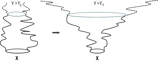
Figure 4.1: For $Y=Y_{c}=-\sqrt{\Lambda}$ the length of the final boundary diverges as $T\rightarrow\infty$.

$$\langle L(T)\rangle_{X,Y,T}=-\frac{1}{G_{\Lambda}(X,Y;T)}\,\frac{\partial G_{\Lambda}(X,Y;T)}{\partial Y}=\frac{1}{{\bar{X}}(T,X)+Y}.$$ (4.8)

With the choice $Y\!=\!-\sqrt{\Lambda}$ one obtains from (4.7) in the limit $T\to\infty$:

$$\langle L(t)\rangle_{X}=\frac{1}{\sqrt{\Lambda}}\;\sinh\left(2\sqrt{\Lambda}(t+t_{0}(X))\right),$$ (4.9)

where $t_{0}(X)$ is defined in eq. (4.4).

We have called $L_{2}$ the (spatial) length of the boundary corresponding to $T$ and $\langle L(t)\rangle_{X}$ the spatial length of a time-slice at time $t$ in order to be in accordance with earlier notation [30, 21], but starting from a lattice regularization and taking the continuum limit $L$ is only determined up to a constant of proportionality which we fix by comparing with a continuum effective action. In section (2.7.3) we showed that such a comparison leads to the identification of $L$ as $L_{cont}/\pi$ and we are led to the following

$$L_{cont}(t)\equiv\pi\langle L(t)\rangle_{X}=\frac{\pi}{\sqrt{\Lambda}}\;\sinh\left(2\sqrt{\Lambda}(t+t_{0}(X))\right).$$ (4.10)

Consider the classical surface where the intrinsic geometry is defined by proper time $t$ and spatial length $L_{cont}(t)$ of the curve corresponding to constant $t$. It has the line element

$$\mbox{d}s^{2}=\mbox{d}t^{2}+\frac{L_{cont}^{2}}{4\pi^{2}}\;\mbox{d}\theta^{2}=\mbox{d}t^{2}+\frac{\sinh^{2}\left(2\sqrt{\Lambda}(t+t_{0}(X))\right)}{4\Lambda}\;\mbox{d}\theta^{2},$$ (4.11)

where $t\geq 0$ and $t_{0}(X)$ is a function of the boundary cosmological constant $X$ at the boundary corresponding to $t\!=\!0$ (see eq. (4.4)). What is remarkable about formula (4.11) is that the surfaces for different boundary cosmological constants $X$ can be viewed as part of the same surface, the Poincaré disc with curvature $R=-8\Lambda$, since $t$ can be continued to $t=-t_{0}$. The Poincaré disc itself is formally obtained in the limit $X\to\infty$ since an infinite boundary cosmological constant will contract the boundary to a point.

4.3 The classical effective action

In this section we make a small digression to the “classical” theory and show that the emergence of the hyperbolic plane is natural from this point of view. In section (2.7.3) we discussed the derivation of the quantum Hamiltonian of causal quantum gravity from the following classical action.

$$S_{\kappa}=\int_{0}^{T}\mbox{d}t\left(\frac{\dot{l}^{2}(t)}{4l(t)}+\Lambda l(t)+\frac{\kappa}{l}\right).$$ (4.12)

To make contact with the inherently quantum calculation by causal dynamical triangulations it is interesting to look at the classical behavior corresponding to this action. The classical solutions corresponding to action (4.12) are

$$l(t) = \frac{\sqrt{\kappa}}{\sqrt{\Lambda}}\;\sinh 2\sqrt{\Lambda}t,\leavevmode\nobreak\ \leavevmode\nobreak\ \leavevmode\nobreak\ \leavevmode\nobreak\ \leavevmode\nobreak\ \leavevmode\nobreak\ \leavevmode\nobreak\ \leavevmode\nobreak\ \leavevmode\nobreak\ \leavevmode\nobreak\ \kappa>0\leavevmode\nobreak\ \leavevmode\nobreak\ \mbox{elliptic case},$$ (4.13)

$$l(t) = \frac{\sqrt{-\kappa}}{\sqrt{\Lambda}}\;\cosh 2\sqrt{\Lambda}t,\leavevmode\nobreak\ \leavevmode\nobreak\ \leavevmode\nobreak\ \leavevmode\nobreak\ \leavevmode\nobreak\ \leavevmode\nobreak\ \leavevmode\nobreak\ \kappa<0\leavevmode\nobreak\ \leavevmode\nobreak\ \mbox{hyperbolic case},$$ (4.14)

$$l(t) = \mbox{e}^{2\sqrt{\Lambda}t},\leavevmode\nobreak\ \leavevmode\nobreak\ \leavevmode\nobreak\ \leavevmode\nobreak\ \leavevmode\nobreak\ \leavevmode\nobreak\ \leavevmode\nobreak\ \leavevmode\nobreak\ \leavevmode\nobreak\ \leavevmode\nobreak\ \leavevmode\nobreak\ \leavevmode\nobreak\ \leavevmode\nobreak\ \leavevmode\nobreak\ \leavevmode\nobreak\ \leavevmode\nobreak\ \leavevmode\nobreak\ \leavevmode\nobreak\ \leavevmode\nobreak\ \leavevmode\nobreak\ \leavevmode\nobreak\ \leavevmode\nobreak\ \leavevmode\nobreak\ \kappa=0\leavevmode\nobreak\ \leavevmode\nobreak\ \mbox{parabolic case},$$ (4.15)

all corresponding to cylinders with constant negative curvature $-8\Lambda$. In the elliptic case, where $t$ must be larger than zero, there is a conical singularity at $t=0$ unless $\kappa=1$. For $\kappa\!=\!1$ the geometry is regular at $t=0$ and this value of $\kappa$ corresponds precisely to the Poincaré disc, $t=0$ being the “center” of the disc. So we see that for $\kappa\!=\!1$ the classical solution coincides nicely with the emergent geometry derived in the previous section

4.4 Quantum fluctuations

In many ways it is more natural to fix the boundary cosmological constant than to fix the length of the boundary. However, one pays the price that the fluctuations of the boundary size are large, in fact of the order of the average length of the boundary itself : from (4.8) we have

$$\langle L^{2}(T)\rangle_{X,Y;T}-\langle L(T)\rangle^{2}_{X,Y;T}=-\frac{\partial\langle L(T)\rangle_{X,Y;T}}{\partial Y}=\langle L(T)\rangle^{2}_{X,Y;T}.$$ (4.16)

Such large fluctuations are also present around $\langle L(t)\rangle_{X,Y;T}$ for $t<T$. From this point of view it is even more remarkable that $\langle L(t)\rangle_{X,Y=-\sqrt{\Lambda};T=\infty}$ has such a nice semiclassical interpretation. Let us now by hand fix the boundary lengths $L_{1}$ and $L_{2}$. This is done in the Hartle-Hawking Euclidean path integral when the geometries $[g]$ are fixed at the boundaries [68]. For our one-dimensional boundaries the geometries at the boundaries are uniquely fixed by specifying the lengths of the boundaries, and the relation between the propagator with fixed boundary cosmological constants and with fixed boundary lengths is given by a Laplace transformation as shown in eq. (4.5). Let us for simplicity analyze the situation where we take the length $L_{1}$ of the entrance loop to zero by taking the boundary cosmological constant $X\to\infty$. Using the decomposition property (4.6) one can calculate the connected “loop-loop” correlator for fixed $L_{2}$ and $0<t\leq t+\Delta<T$,

$$\langle L(t)L(t+\Delta)\rangle^{(c)}_{L_{2},T}\equiv\langle L(t+\Delta)L(t)\rangle_{L_{2},T}-\langle L(t)\rangle\langle L(t+\Delta)\rangle_{L_{2},T}.$$ (4.17)

One finds

$$\langle L(t)L(t\!+\!\Delta)\rangle^{(c)}_{L_{2},T} = \frac{2}{\Lambda}\frac{\sinh^{2}\sqrt{\Lambda}t\sinh^{2}\sqrt{\Lambda}(T\!-\!(t\!+\!\Delta))}{\sinh^{2}\sqrt{\Lambda}T}+$$

$$\frac{2L_{2}}{\sqrt{\Lambda}}\frac{\sinh^{2}\sqrt{\Lambda}t\sinh\sqrt{\Lambda}(t\!+\!\Delta)\sinh\sqrt{\Lambda}(T\!-\!(t\!+\!\Delta))}{\sinh^{3}\sqrt{\Lambda}T}.$$

We also note that

$$\langle L(t)\rangle_{L_{2},T}=\frac{2}{\sqrt{\Lambda}}\frac{\sinh\sqrt{\Lambda}t\sinh\sqrt{\Lambda}(T\!-\!t)}{\sinh\sqrt{\Lambda}T}+L_{2}\frac{\sinh^{2}\sqrt{\Lambda}t}{\sinh^{2}\sqrt{\Lambda}T}.$$ (4.19)

For fixed $L_{2}$ and $T\to\infty$ we obtain

$$\langle L(t)L(t+\Delta)\rangle^{(c)}_{L_{2}}=\frac{1}{2\Lambda}\;\mbox{e}^{-2\sqrt{\Lambda}\Delta}\left(1-\mbox{e}^{-2\sqrt{\Lambda}t}\right)^{2}$$ (4.20)

and

$$\langle L(t)\rangle_{L_{2}}=\frac{1}{\sqrt{\Lambda}}\left(1-\mbox{e}^{-2\sqrt{\Lambda}t}\right).$$ (4.21)

Eqs. (4.20) and (4.21) tell us that except for small $t$ we have $\langle L(t)\rangle_{L_{2}}\!=\!1/\sqrt{\Lambda}$. The quantum fluctuations $\Delta L(t)$ of $L(t)$ are defined by $(\Delta L(t))^{2}=\langle L(t)L(t)\rangle^{(c)}$. Thus the spatial extension of the universe is just quantum size (i.e.  $1/\sqrt{\Lambda}$, $\Lambda$ being the only coupling constant) with fluctuations $\Delta L(t)$ of the same size. The time correlation between $L(t)$ and $L(t+\Delta)$ is also dictated by the scale $1/\sqrt{\Lambda}$, telling us that the correlation between spatial elements of size $1/\sqrt{\Lambda}$, separated in time by $\Delta$ falls of exponentially as $e^{-2\sqrt{\Lambda}\Delta}$ . The above picture is precisely what one would expect from the classical action, which is proportional to the area and the boundary cosmological constants only, if we force $T$ to be large and choose a $Y$ such that $\langle L_{2}(T)\rangle$ is not large, the universe will be a thin tube, “classically” of zero width, but due to quantum fluctuations of average width $1/\sqrt{\Lambda}$.

A more interesting situation is obtained if we choose $Y=-\sqrt{\Lambda}$, the special value needed to obtain a non-compact geometry in the limit $T\to\infty$. To implement this in a setting where $L_{2}$ is not allowed to fluctuate we fix $L_{2}(T)$ to the average value (4.8) for $Y\!=\!\!-\!\sqrt{\Lambda}$:

$$L_{2}(T)=\langle L(T)\rangle_{X,Y=-\sqrt{\Lambda};T}=\frac{1}{\sqrt{\Lambda}}\;\frac{1}{\coth\sqrt{\Lambda}T-1}.$$ (4.22)

From (4.4) and (4.19) we have in the limit $T\to\infty$:

$$\langle L(t)\rangle=\frac{1}{\sqrt{\Lambda}}\;\sinh 2\sqrt{\Lambda}t,$$ (4.23)

in accordance with (4.9), and for the “loop-loop”-correlator

$$\langle L(t+\Delta)L(t)\rangle^{(c)}=\frac{2}{\Lambda}\;\sinh^{2}\sqrt{\Lambda}t=\frac{1}{\sqrt{\Lambda}}\left(\langle L(t)\rangle-\frac{1}{\sqrt{\Lambda}}\left(1-\mbox{e}^{-2\sqrt{\Lambda}t}\right)\right).$$ (4.24)

It is seen that the “loop-loop”-correlator is independent of $\Delta$. In particular we have for $\Delta\!=\!0$:

$$(\Delta L(t))^{2}\equiv\langle L^{2}(t)\rangle-\langle L(t)\rangle^{2}\sim\frac{1}{\sqrt{\Lambda}}\langle L(t)\rangle$$ (4.25)

for $t\gg 1/\sqrt{\Lambda}$. The interpretation of eq. (4.25) is in accordance with the picture presented below (4.21): We can view the curve of length $L(t)$ as consisting of $N(t)\approx\sqrt{\Lambda}L(t)\approx e^{2\sqrt{\Lambda}t}$ independently fluctuating parts of size $1/\sqrt{\Lambda}$ and each with a fluctuation of size $1/\sqrt{\Lambda}$. Thus the total fluctuation $\Delta L(t)$ of $L(t)$ will be of order $1/\sqrt{\Lambda}\times\sqrt{N(t)}$,

$$\frac{\Delta L(t)}{\langle L(t)\rangle}\sim\frac{1}{\sqrt{\sqrt{\Lambda}\langle L(t)\rangle}}\sim\mbox{e}^{-\sqrt{\Lambda}t},$$ (4.26)

i.e. the fluctuation of $L(t)$ around $\langle L(t)\rangle$ is small for $t\gg 1/\sqrt{\Lambda}$. In the same way the independence of the “loop-loop”-correlator of $\Delta$ can be understood as the combined result of $L(t+\Delta)$ growing exponentially in length with a factor $e^{2\sqrt{\Lambda}\Delta}$ compared to $L(t)$ and, according to (4.20), the correlation of “line-elements” of $L(t)$ and $L(t+\Delta)$ decreasing by a factor $e^{-2\sqrt{\Lambda}\Delta}$.

4.5 Summary

We have described how the CDT quantization of 2d gravity for a special value of the boundary cosmological constant leads to a non-compact (Euclidean) AdS-like spacetime of constant negative curvature dressed with quantum fluctuations. It is possible to achieve this non-compact geometry as a limit of a compact geometry as described above. In particular the assignment (4.22) leads to a simple picture where the fluctuation of $L(t)$ is small compared to the average value of $L(t)$. In fact the geometry can be viewed as that of the Poincaré disc with fluctuations correlated only over a distance $1/\sqrt{\Lambda}$.

Our construction is similar to the analysis of $ZZ$-branes appearing as a limit of compact 2d geometries in Liouville quantum gravity [66]. In the CDT case the non-compactness came when the running boundary cosmological constant ${\bar{X}}(T)$ went to the fixed point $\sqrt{\Lambda}$ for $T\to\infty$. In the case of Liouville gravity, represented by DT (or equivalently matrix models), the non-compactness arose when the running (Liouville) boundary cosmological constant ${{\bar{X}}_{Liouville}(T)}$ went to the value where the disc amplitude $W_{\tilde{\Lambda}}({\tilde{X}})\!=\!0$, i.e. to ${\tilde{X}}\!=\!\sqrt{{\tilde{\Lambda}}}/2$ (see eq. (4.1)). It is the same process in the two cases, since the relation between Liouville gravity and CDT is well established and summarized by the mapping [31]:

$$\frac{X}{\sqrt{\Lambda}}=\sqrt{\frac{2}{3}}\;\sqrt{1+\frac{{\tilde{X}}}{\sqrt{{\tilde{\Lambda}}}}},$$ (4.27)

between the coupling constants of the two theories. The physical interpretation of this relation is discussed in [31, 21]: One obtains the CDT model by chopping away all baby-universes from the Liouville gravity theory, i.e. universes connected to the “parent-universe” by a worm-hole of cut-off scale, and this produces the relation (4.27) . It is seen that $X\to\sqrt{\Lambda}$ corresponds precisely to $\tilde{X}\to\sqrt{{\tilde{\Lambda}}}/2$.

While the starting point of the CDT quantization was the desire to include only Lorentzian, causal geometries in the path integral, the result (4.11) shows that after rotation to Euclidean signature this prescription is in a natural correspondence with the Euclidean Hartle-Hawking no-boundary condition, since all of the geometries (4.11) have a continuation to $t\!=\!-t_{0}$, where the spacetime is regular. It would be interesting if this could be promoted to a general principle also in higher dimensions. The computer simulations reported in [24, 25, 26, 27, 28, 29] seem in accordance with this possibility.

Chapter 5 Topology fluctuations of space and time

In this chapter we refocus our attention on the issue of topology change in quantum gravity. We make some steps to go beyond the results of chapter 3 and incorporate topology fluctuations of space and time in the path integral of two dimensional CDT. In field theory language one would say that in this chapter we go beyond tree level by computing loop corrections. The incorporation of loop corrections is a notoriously difficult undertaking however. Even in standard quantum field theory the loop expansion is not convergent so one can only validly utilize the perturbation theory up to a limited number of loops. Technically, the expansion merely forms an asymptotic power series instead of a convergent one. The basic reason behind the divergence of the series expansion is that for large number of loops the amount of diagrams grows super-exponentially.

The situation for gravity is typically similar, the number of ways in which one can cut and reglue a manifold to obtain manifolds with a different topology is very large and leads to uncontrollable divergences in the path integral. Even in the simplest case of two dimensional Euclidean geometries, the number of possible configurations grows faster than exponentially with the volume of the geometry. A well-known manifestation of this problem is the non-Borel summability of the genus expansion in string theory. This does not necessarily mean that there is no underlying well-defined theory, but even in the much-studied case of two dimensional Euclidean quantum gravity no physically satisfactory, unambiguous solution has been found [18].

Our contribution to the problem of spacetime topology change is twofold. In section (5.1) we take a modest point of view and analyze the issue of spacetime topology change perturbatively in the loop expansion. Particularly, we expand the standard formalism of two dimensional causal quantum gravity and compute the Hartle Hawking wavefunction up to second order in the genus expansion. The statistical mechanics of loop diagrams is considerably more complicated than the tree diagrams that were analyzed in chapter 3 henceforh we are not be able to address the summability of the expansion.

On a more positive and perhaps more speculative note we introduce a toy model in section (5.2) where we show that it might be possible to define a nonperturbative sum over topologies provided suitable causality restrictions are imposed . This section is based on [72].

5.1 Perturbation theory

Recall that the time dependent disc amplitude of pure CDT is given by

$$W_{\Lambda}(L,T)=\frac{\Lambda}{\sinh^{2}\sqrt{\Lambda}T}e^{{-\sqrt{\Lambda}L\coth\sqrt{\Lambda}T}}$$ (5.1)

which is obtained from the propagator by shrinking the initial boundary to a point, i.e.  $W_{\Lambda}(L,T)\!=\!G_{\Lambda}(L_{1}\!=\!0,L;T)$. Upon integrating over time one obtains the Hartle Hawking wavefunction,

$$W_{\Lambda}(L)=\int_{0}^{\infty}dT\;W_{\Lambda}(L,T)=\frac{e^{-\sqrt{\Lambda}L}}{L}.$$ (5.2)

To go beyond this genus zero result we need to extend the existing literature on two dimensional CDT by computing amplitudes where the spatial topology is allowed to change. A simple example of such an object is the before mentioned trouser amplitude (fig. 5.1). It can be obtained by “gluing” three cylinder amplitudes. In this gluing procedure one takes a propagator with a final loop length $(L+L^{\prime})$ that is equal to the sum of the lengths of the initial loops $L$ and $L^{\prime}$ of two other propagators and integrates over $L$ and $L^{\prime}$. As in the case of the composition rule (2.32) one has to include a measure factor to obtain the correct amplitudes. Furthermore, from a continuum perspective one can say that the gluing is defined such that Dehn twists around spatial slices are not present. Instead of writing out the measure factors explicitly we absorb them into the propagators by marking the loops of the amplitudes that are being glued. For convenience we also use a mixed representation for the propagators where one of the boundaries has fixed cosmological constant and the other has fixed boundary length,

$$G_{\Lambda}(X,L,T)=\frac{e^{-\bar{X}_{X}(T)L}}{L}-\frac{e^{-L\bar{X}_{\infty}(T)}}{L}$$ (5.3)

where $\bar{X}_{X}(T)$ is given by

$$\bar{X}_{X}(T)=\bar{X}_{\infty}(T)-\frac{\Lambda}{\sinh^{2}\sqrt{\Lambda}T\left(X+\bar{X}_{\infty}(T)\right)}$$ (5.4)

and $\bar{X}_{\infty}(T)\!=\!\sqrt{\Lambda}\coth\sqrt{\Lambda}T$.

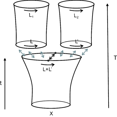
Figure 5.1: Elementary trouser amplitude by gluing propagators

We can now calculate the trouser amplitude from an initial boundary with boundary cosmological constant $X$ to two final boundaries of length $L_{1}$ and $L_{2}$ in time $T$, where the splitting occurs after a fixed time $t$ (fig. 5.1),

$${\cal T}_{\Lambda}(X,L_{1},L_{2};T,t)\! = \!2\!\int\limits^{\infty}_{0}\int\limits^{\infty}_{0}dLdL^{\prime}G_{\Lambda}^{(0;1)}\!(X,L\!+\!L^{\prime},t)\times$$ (5.5)

$$G_{\Lambda}^{(1;0)}\!(L,L_{1},T\!-\!t)G_{\Lambda}^{(1;0)}\!(L^{\prime},L_{2},T\!-\!t),$$

where the superscript notation of the propagators denotes the marking of its loops, as introduced in section (2.7.2). Performing the integrations yields

$${\cal T}_{\Lambda}(X,L_{1},L_{2};T,t) = 2\leavevmode\nobreak\ e^{-\bar{X}_{X}(T)(L_{1}+L_{2})}\left(\frac{\sqrt{\Lambda}\cosh\sqrt{\Lambda}t+X\sinh\sqrt{\Lambda}t}{\sqrt{\Lambda}\cosh\sqrt{\Lambda}T+X\sinh\sqrt{\Lambda}T}\right)^{4}$$ (5.6)

$$\!+\leavevmode\nobreak\ 2\leavevmode\nobreak\ e^{-\bar{X}_{\infty}(t)(L_{1}+L_{2})}\!\left(\frac{\sinh\sqrt{\Lambda}t}{\sinh\sqrt{\Lambda}T}\right)^{4}.$$

In the rest of the section we only present results where the length of the initial loop is zero to keep the presentation as transparent as possible. The trouser amplitude with zero initial length is dubbed the splitting amplitude which we denote by ${\cal S}$. In particular we are interested in the splitting amplitude to two final loops of length $L_{1}$ and $L_{2}$, where the time before the splitting is arbitrary and the time after the splitting is fixed to be $t^{\prime}$

$${\cal S}_{\Lambda}(L_{1},L_{2};t^{\prime}) = 2\int\limits^{\infty}_{0}dL\int\limits^{\infty}_{0}dL^{\prime}\,W_{\Lambda}^{(1)}(L+L^{\prime})G_{\Lambda}^{(1;0)}(L,L_{1};t^{\prime})G_{\Lambda}^{(1;0)}(L^{\prime},L_{2};t^{\prime})$$ (5.7)

$$= 2\,e^{-(L1+L2)\sqrt{\Lambda}}e^{-4t^{\prime}\sqrt{\Lambda}}.$$

This amplitude might seem a bit unnatural, since it treats the time intervals before and after splitting differently. It is however useful for studying averages of the duration of a hole (section (5.1.1)). If we integrate over the time after the split in spatial topology as well we obtain

$${\cal S}_{\Lambda}(L_{1},L_{2})=\int\limits^{\infty}_{0}dt^{\prime}{\cal S}_{\Lambda}(L_{1},L_{2};t^{\prime})=\frac{e^{-(L1+L2)\sqrt{\Lambda}}}{2\sqrt{\Lambda}}.$$ (5.8)

In the following we use the results obtained in this subsection to calculate higher genus Hartle Hawking wavefunctions within our model.

5.1.1 Higher genus Hartle Hawking wavefunctions

In this section we present genus one and genus two generalizations of the Hartle Hawking wave function where we integrate over the time intervals. It is possible to obtain results where the time intervals are fixed, but we choose to omit them for sake of clarity. Given the splitting amplitude (5.8) it is straightforward to compute the genus one generalization of the Hartle Hawking wavefunction (5.2). To simplify calculations we first obtain the genus one wave function with fixed boundary cosmological constant $Y$ and a mark on the boundary (see fig. 5.2),

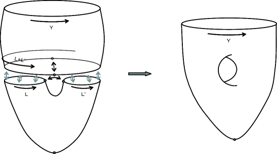
Figure 5.2: Construction of the genus one disc function from the splitting amplitude and a propagator.

$$W^{(1)}_{\Lambda,{\mathfrak{g}}=1}(Y)=e^{-2\kappa}\int\limits^{\infty}_{0}dL\int\limits^{\infty}_{0}dL^{\prime}{\cal S}_{\Lambda}^{(1,1)}(L,L^{\prime})G^{(1;1)}_{\Lambda}(L+L^{\prime},Y),$$ (5.9)

where $\kappa\!=\!2\pi/G^{b}_{N}$ is proportional to the inverse bare Newton’s constant and ${\cal S}^{(1,1)}$ denotes that both loops of the splitting amplitude possess a mark. Since 2D quantum gravity can be viewed as string theory with a zero dimensional target space, $e^{-\kappa}$ can be identified with a bare string coupling $g_{s}$. The renormalization of this coupling is addressed in the next section. Performing the integrations in (5.9) one obtains

$$W^{(1)}_{\Lambda,{\mathfrak{g}}=1}(Y)=g^{2}_{s}\frac{Y^{3}+5\sqrt{\Lambda}Y^{2}+11\Lambda Y+15\Lambda^{3/2}}{32\left(Y+\sqrt{\Lambda}\right)^{5}\Lambda^{5/2}}.$$ (5.10)

If we now do an inverse Laplace transformation from $Y$ to $L$ and divide by $L$ to remove the mark, we obtain the desired genus one Hartle Hawking wave function,

$$W_{\Lambda,{\mathfrak{g}}=1}(L)=g^{2}_{s}\frac{e^{-L\sqrt{\Lambda}}\left(\Lambda^{3/2}L^{3}+2\Lambda L^{2}+3\sqrt{\Lambda}L+3\right)}{96\Lambda^{5/2}}.$$ (5.11)

One can use the previous results to compute simple observables. For example, using (5.7) we can obtain the average duration of the hole in the genus one disc amplitude:

$$\left<t\right>_{\text{hole}} = \frac{1}{W^{(1)}_{\Lambda,{\mathfrak{g}}=1}(Y)}\int\limits^{\infty}_{0}dt^{\prime}\,t^{\prime}\int\limits^{\infty}_{0}dL\int\limits^{\infty}_{0}dL^{\prime}{\cal S}_{\Lambda}^{(1,1)}(L,L^{\prime};t^{\prime})G^{(1;1)}_{\Lambda}(L+L^{\prime},Y)$$ (5.12)

$$= \frac{1}{4\sqrt{\Lambda}}.$$

The size of the hole is determined by $1/\sqrt{\Lambda}$ which is the only length scale in the model. Similarly we get for the fluctuations

$$\left<\Delta t\right>_{\text{hole}}=\sqrt{\left<t^{2}\right>_{\text{hole}}-\left<t\right>_{\text{hole}}^{2}}=\frac{1}{4\sqrt{\Lambda}}.$$ (5.13)

It is interesting to observe that $\left<\Delta t\right>_{\text{hole}}\!=\!\left<t\right>_{\text{hole}}$. This reflects the fact that as for the spatial geometry, where we have $\left<\Delta L\right>\!\sim\!\left<L\right>$, the geometry of the holes is also purely governed by quantum fluctuations.

The procedure to obtain the genus two wave function is analogous to the one outlined above. In practice it involves doing much more tedious calculations however, since one has to glue more and more propagators. This does not introduce any fundamental complications and does not give one much more physical insight so we only present the result of the computations. To obtain the genus two wave function one needs to add contributions from three different diagrams,

$$W_{\Lambda,{\mathfrak{g}}=2}(L)=W^{a}_{\Lambda,{\mathfrak{g}}=2}(L)+W^{b}_{\Lambda,{\mathfrak{g}}=2}(L)+W^{c}_{\Lambda,{\mathfrak{g}}=2}(L)=\raisebox{-20.0pt}{\includegraphics[height=45.0pt]{Wg2a}}+\raisebox{-20.0pt}{\includegraphics[height=45.0pt]{Wg2b}}+\raisebox{-20.0pt}{\includegraphics[height=45.0pt]{Wg2c}}$$ (5.14)

which evaluates to,

$$W_{\Lambda,{\mathfrak{g}}=2}(l)=g^{4}_{s}{\textstyle\frac{e^{-l}\left(3l^{7}+28l^{6}+150l^{5}+570l^{4}+1575l^{3}+3150l^{2}+4725l+4725\right)}{92160\Lambda^{11/2}}},$$ (5.15)

where the dimensionless variable $l=L\sqrt{\Lambda}$ is the length of the boundary in units of $\sqrt{\Lambda}$.

Double scaling limit

Looking at the Hartle Hawking wave functions for genus ${\mathfrak{g}}=0,1,2$ , i.e.  Eqs. (5.2), (5.11) and (5.15), one can see that they all have different dimensions. Specifically, the ${\mathfrak{g}}=0,1,2$ wave functions have dimension of $\Lambda^{1/2}$, $\Lambda^{-5/2}$ and $\Lambda^{-11/2}$ respectively. This would imply that the different genus contributions cannot be added to a single wave function. In fact one can add them if one takes into account their wave function renormalization factors that appear when taking the continuum limit of the discrete sums. The reason why those factors did not appear in the previous sections is that for the case of fixed topology one absorbs these factors in the boundary states of the theory. If one would have kept those factors from the outset the ${\mathfrak{g}}=0,1,2$ wave functions would all be dimensionless and would behave as $a\sqrt{\Lambda}$, $(a\sqrt{\Lambda})^{-5}$ and $(a\sqrt{\Lambda})^{-11}$ respectively, where $a$ is the cutoff of the theory induced by the discrete lattice spacing.

To remove this cutoff dependence on the lattice spacing $a$ one can do a renormalization of the string coupling such that all higher genus diagrams will contribute in the continuum limit. The simultaneous scaling of the string coupling and the cosmological constant is called the “double scaling” limit. In particular, we obtain

$$g_{S}=g_{s}(a\sqrt{\Lambda})^{3}.$$ (5.16)

Observe that this scaling limit is the same as the scaling we considered in chapter 3. This implies that the spatial and spacetime topology changes are in fact part of one topological expansion. Using this scaling limit we can now derive the Hartle Hawking wave function up to order two in the genus expansion,

$$\!\!\!\!\!\!\!\!\!W_{\Lambda,g_{S}}(l)\!\!\! = \!\!\!{\textstyle\sqrt{\Lambda}\,e^{-l}\left(\frac{1}{l}+g^{2}_{S}\frac{l^{3}+2l^{2}+3l+3}{96}+\right.}$$

$$\,\,\,\,\,\,\,\,{\textstyle\left.+g_{S}^{4}{\textstyle\frac{e^{-l}\left(3l^{7}+28l^{6}+150l^{5}+570l^{4}+1575l^{3}+3150l^{2}+4725l+4725\right)}{92160}}+\mathcal{O}(g_{S}^{6})\right),}$$

where we again used the dimensionless variable $l=L\sqrt{\Lambda}$.

5.1.2 Summary

We have described how to include manifolds of higher genus in the path integral of two dimensional CDT. One of the main results is the computation of the Hartle Hawking wave function up to two loops in the genus expansion. Generalization to higher genus is in principle straightforward, however, the calculations become more and more cumbersome. It is interesting to note that the Hartle Hawking wave functions in the framework of CDT are very similar to the Hartle Hawking amplitudes in Euclidian Dynamical Triangulations [18]. Using the method of loop equations it is possible to also obtain higher genus results for 2D Euclidean quantum gravity [47, 48]. A detailed comparison of these results might lead to a better understanding of the relationship between Euclidean and Lorentzian quantum gravity.

5.2 Nonperturbative sum over topologies?

As shown in previous work, there is a well-defined nonperturbative gravitational path integral including an explicit sum over topologies in the setting of causal dynamical triangulations in two dimensions. In this section we derive a complete analytical solution of the quantum continuum dynamics of this model, obtained uniquely by means of a double-scaling limit. We show that the presence of infinitesimal wormholes leads to a decrease of the effective cosmological constant, reminiscent of the suppression mechanism considered by Coleman and others in the four-dimensional Euclidean path integral. Remarkably, in the continuum limit we obtain a finite spacetime density of microscopic wormholes without assuming fundamental discreteness. This shows that one can in principle make sense of a gravitational path integral which includes a sum over spacetime topologies, provided suitable causality restrictions are imposed on the path integral histories.

5.2.1 Outline

A new idea to tame the divergences associated with spacetime topology changes in the path integral was advanced in [73] and implemented in a model of two dimensional nonperturbative Lorentzian quantum gravity. The idea is to include a sum over topologies, or over some subclass of topologies, in the state sum, but to restrict this class further by certain geometric (as opposed to topological) constraints. These constraints involve the causal (and therefore Lorentzian) structure of the spacetimes and thus would have no analogue in a purely Euclidean formulation. In the concrete two dimensional model considered in [73], the path integral is taken over a geometrically distinguished class of spacetimes with arbitrary numbers of “wormholes”, which violate causality only relatively mildly (see also [74]). As a consequence, the nonperturbative path integral turns out to be well defined. This is an extension of the central idea of the approach of causal dynamical triangulations, namely, to use physically motivated causality restrictions to make the gravitational path integral better behaved (see [75] for a review).

In section (5.2.3), we will present a complete analytical solution of the statistical model of two dimensional Lorentzian random geometries introduced in [73], whose starting point is a regularized sum over causal triangulated geometries including a sum over topologies. For a given genus (i.e. number of (worm)holes in the spacetime) not all possible triangulated geometries are included in the sum, but only those which satisfy certain causality constraints. As shown in [73], this makes the statistical model well defined, and an unambiguous continuum limit is obtained by taking a suitable double-scaling limit of the two coupling constants of the model, the gravitational or Newton’s constant and the cosmological constant. The double-scaling limit presented here differs from the one found in [73, 74], where only the partition function for a single spacetime strip was evaluated. We will show that when one includes the boundary lengths of the strip explicitly – as is necessary to obtain the full spacetime dynamics – the natural renormalization of Newton’s constant involves the boundary “cosmological” coupling constants conjugate to the boundary lengths. Although the holes we include exist only for an infinitesimal time, and we do not keep track of them explicitly in the states of the Hilbert space, their integrated effect is manifest in the continuum Hamiltonian of the resulting gravity theory. As we will see, their presence leads to an effective lowering of the cosmological constant and therefore represents a concrete and nonperturbative implementation of an idea much discussed in the late eighties in the context of the ill-defined continuum path integral formulation of Euclidean quantum gravity (see, for example, [76, 77]).

The remainder of this section is structured as follows. In the next subsection, we briefly describe how a nonperturbative theory of two dimensional Lorentzian quantum gravity can be obtained by the method of causal dynamical triangulation (CDT), and how a sum over topologies can be included. For a more detailed account of the construction of topology-changing spacetimes and the geometric reasoning behind the causality constraints we refer the reader to [73, 74]. The main result of Sec. (5.2.3) is the computation of the Laplace transform of the one-step propagator of the discrete model for arbitrary boundary geometries. In Sec. (5.2.4) we make a scaling ansatz for the coupling constants and show that just one of the choices for the scaling of Newton’s constant leads to a new and physically sensible continuum theory. We calculate the corresponding quantum Hamiltonian and its spectrum, as well as the full propagator of the theory. Using these results, we compute several observables of the continuum theory in Sec. (5.2.5), most importantly, the expectation value of the number of holes and its spacetime density. In Sec. (5.2.6), we summarize our results and draw a number of conclusions. In Appendix B, we discuss the properties of alternative scalings for Newton’s constant which were discarded in the main text. This also establishes a connection with previous attempts [78, 79] to generalize the original Lorentzian model without topology changes. In Appendix C, we calculate the spacetime density of holes from a single infinitesimal spacetime strip.

5.2.2 Implementing the sum over topologies

Our aim is to calculate the (1+1) -dimensional gravitational path integral

$$Z(G_{N},\Lambda)=\sum_{topol.}\int D[g_{\mu\nu}]e^{iS(g_{\mu\nu})}$$ (5.18)

nonperturbatively by using the method of Causal Dynamical Triangulations (CDT). The sum in (5.18) denotes the inclusion in the path integral of a specific, causally preferred class of fluctuations of the manifold topology. The action $S(g_{\mu\nu})$ consists of the usual Einstein-Hilbert curvature term and a cosmological constant term. Since we work in two dimensions, we recall that integrated curvature term is proportional to the Euler characteristic $\chi=2\!-\!2{\mathfrak{g}}\!-\!b$ of the spacetime manifold, where ${\mathfrak{g}}$ denotes the genus (i.e. the number of handles or holes) and $b$ the number of boundary components. Explicitly, the action reads

$$S=2\pi\chi K-\Lambda\int d^{2}x\sqrt{|\det g_{\mu\nu}|},$$ (5.19)

where $K=1/G_{N}$ is the inverse Newton’s constant and $\Lambda$ the cosmological constant (with dimension of inverse length squared).

Just like in the original CDT model [21] we will first regularize the path integral (5.18) by a sum over piecewise flat two dimensional spacetimes, whose flat building blocks are identical Minkowskian triangles, all with one spacelike edge of squared length $+a^{2}$ and two timelike edges of squared length $-\alpha a^{2}$, where $\alpha$ is a real positive constant. The CDT path integral takes the form of a sum over triangulations, with each triangulation consisting of a sequence of spacetime strips of height $\Delta t=1$ in the time direction. A single such strip is a set of $l_{1}$ triangles pointing up and $l_{2}$ triangles pointing down (fig. 2.7). Because the geometry has a sliced structure, one can easily Wick-rotate it to a triangulated manifold of Euclidean signature by analytically continuing the parameter $\alpha$ to a real negative value [80]. For simplicity, we will set $\alpha\!=\!-1$ in evaluating the regularized, real and Wick-rotated version of the path integral (5.18).

In the pure CDT model the one-dimensional spatial slices of constant proper time $t$ are usually chosen as circles, resulting in cylindrical spacetime geometries. For our present purposes, we will enlarge this class of geometries by allowing the genus to be variable. We define the sum over topologies by performing surgery moves directly on the triangulations to obtain regularized versions of higher-genus manifolds [73, 74]. They are generated by adding tiny wormholes that connect two regions of the same spacetime strip. Starting from a regular strip of topology $[0,1]\times S^{1}$ and height $\Delta t=1$, one can construct a hole by identifying two of the strip’s timelike edges and subsequently cutting open the geometry along this edge (fig. 5.3). By applying this procedure repeatedly (obeying certain causality constraints [73, 74]), more and more wormholes can be created. Once the regularized path integral has been performed, including a sum over geometries with wormholes, one takes a continuum limit by letting $a\rightarrow 0$ and renormalizing the coupling constants appropriately, as will be described in the following sections.

Note that our wormholes are minimally causality- and locality-violating in that they are located within a single proper-time step (the smallest time unit available in the discretized theory) and the associated baby universes which are born at time $t$ are reglued at time $t+1$ “without twist” [73, 74]. In a macroscopic interpretation one could describe them as wormholes which are instantaneous in the proper-time frame of an ensemble of freely falling observers. Note that this is invariantly defined (on Minkowski space, say) once an initial surface has been chosen. Such a restriction is necessary if one wants to arrive at a well-defined unitary evolution via a transfer matrix formalism, as we are doing. To include wormholes whose ends lie on different proper-time slices, one would have to invoke a third-quantized formulation, which would very likely result in macroscopic violations of causality, locality and therefore unitarity, something we are trying to avoid in the present model.

One could wonder whether the effect in the continuum theory of our choice of wormholes is to single out a preferred coordinate system. Our final result will show that this is not the case, at least not over and above that of the pure gravitational model without topology changes. The effect of the inclusion of wormholes turns out to be a rather mild “dressing” of the original theory without holes. We believe that the essence of our model lies not so much in how the wormholes are connected, because they do not themselves acquire a nontrivial dynamics in the continuum limit. Rather, it is important that their number is sufficiently large to have an effect on the underlying geometry, but on the other hand sufficiently controlled so as to render the model computable.

A similar type of wormhole has played a prominent role in past attempts to devise a mechanism to explain the smallness of the cosmological constant in the Euclidean path integral formulation of four-dimensional quantum gravity in the continuum [76, 77]. The wormholes considered there resemble those of our toy model in that both are non-local identifications of the spacetime geometry of infinitesimal size. The counting of our wormholes is of course different since we are working in a genuinely Lorentzian setup where certain causality conditions have to be fulfilled. This enables us to do the sum over topologies completely explicitly. Whether a similar construction is possible also in higher dimensions is an interesting, but at this stage open question.

5.2.3 Discrete solution: the one-step propagator

For the (1+1) -dimensional Lorentzian gravity model including a sum over topologies, the partition function of a single spacetime strip of infinitesimal duration with summed-over boundaries was evaluated in [73] and [74]. In the present section, we will extend this treatment by calculating the full one-step propagator, or, equivalently, the generating function for the partition function of a single strip with given, fixed boundary lengths. This opens the way for investigating the full dynamics of the model.

Figure 5.3: Construction of a wormhole by identifying two timelike edges of a spacetime strip and cutting open the geometry along the edge.

The discrete set-up described above leads to the Wick-rotated one-step propagator

$$G_{\lambda,\kappa}(l_{1},l_{2},t=1)=e^{-\lambda(l_{1}+l_{2})}\sum_{T|l_{1},l_{2}}e^{-2\kappa{\mathfrak{g}}},$$ (5.20)

where $\kappa$ is the bare inverse Newton’s constant and $\lambda$ the bare (dimensionless) cosmological constant, and we have omitted an overall constant coming from the Gauss-Bonnet integration. The sum in (5.20) is to be taken over all triangulations with $l_{1}$ spacelike links in the initial and $l_{2}$ spacelike links in the final boundary. Note that the number of holes does not appear as one of the arguments of the one-step propagator since we only consider holes that exist within one strip. Consequently, the number of holes does not appear explicitly as label for the quantum states, and the Hilbert space coincides with that of the pure CDT model. Nevertheless, the integrated effect of the topologically non-trivial configurations changes the dynamics and the quantum Hamiltonian, as we shall see.

The one-step propagator (5.20) defines a transfer matrix $\hat{T}$ by

$$G_{\lambda,\kappa}(l_{1},l_{2},1)=\langle l_{2}|\hat{T}|l_{1}\rangle,$$ (5.21)

from which we obtain the propagator for $t$ time steps as usual by iteration,

$$G_{\lambda,\kappa}(l_{1},l_{2},t)=\langle l_{2}|\hat{T}^{t}|l_{1}\rangle.$$ (5.22)

For simplicity we perform the sum in (5.20) over triangulated strips with periodically identified boundaries in the spatial direction and one marked timelike edge. By virtue of the latter, $G_{\lambda,\kappa}(l_{1},l_{2},t)$ satisfies the desired composition property of a propagator,

$$G_{\lambda,\kappa}(l_{1},l_{2},t_{1}+t_{2}) = \sum_{l}G_{\lambda,\kappa}(l_{1},l,t_{1})G_{\lambda,\kappa}(l,l_{2},t_{2}),$$ (5.23)

$$G_{\lambda,\kappa}(l_{1},l_{2},t+1) = \sum_{l}G_{\lambda,\kappa}(l_{1},l,1)G_{\lambda,\kappa}(l,l_{2},t),$$ (5.24)

where the sums on the right-hand sides are performed over an intermediate constant-time slice of arbitrary discrete length $l$.

Performing the fixed-genus part of the sum over triangulations in (5.20) yields

$$G_{\lambda,\kappa}(l_{1},l_{2},1)=e^{-\lambda N}\sum_{{\mathfrak{g}}=0}^{[N/2]}\binom{N}{l_{1}}\binom{N}{2{\mathfrak{g}}}\frac{(2{\mathfrak{g}})!}{{\mathfrak{g}}!({\mathfrak{g}}+1)!}e^{-2\kappa{\mathfrak{g}}},$$ (5.25)

with $N\!=\!l_{1}\!+\!l_{2}$. To simplify calculations we will use the generating function formalism with

$$G(x,y,g,h,1)=\sum_{l_{1},l_{2}=0}^{\infty}G_{\lambda,\kappa}(l_{1},l_{2},1)x^{l_{1}}y^{l_{2}},$$ (5.26)

where we have defined $g\!=\!e^{-\lambda}$ and $h\!=\!e^{-\kappa}$. The quantities $x$ and $y$ can be seen as purely technical devices, or alternatively as exponentiated bare boundary cosmological constants

$$x=e^{-\lambda_{in}},\quad y=e^{-\lambda_{out}}.$$ (5.27)

Upon evaluating the sum over $l_{1}$ and $l_{2}$ one obtains the generating function of the one-step propagator

$$G(x,y,g,h,1)=\frac{1}{1-g\,\left(x+y\right)}\frac{2}{1+{\sqrt{1-4u^{2}}}},$$ (5.28)

with

$$u=\frac{h}{\frac{1}{g\,\left(x+y\right)}-1}.$$ (5.29)

Note that in order to arrive at the final result (5.28), we have performed an explicit sum over all topologies! The fact that this infinite sum converges for appropriate values of the bare couplings has to do with the causality constraints imposed on the model, which were geometrically motivated in [73], and which effectively reduce the number of geometries in the genus expansion.

In (5.28) one recognizes the generating function ${\rm Cat}(u^{2})$ for the Catalan numbers,

$${\rm Cat}(u^{2})=\frac{2}{1+{\sqrt{1-4u^{2}}}}.$$ (5.30)

For $h\!=\!0$ one has ${\rm Cat}(u^{2})\!=\!1$ and expression (5.28) reduces to the one-step propagator without topology changes,

$$G(x,y,g,h=0,1)=\frac{1}{1-g\,\left(x+y\right)}.$$ (5.31)

Furthermore, one recovers the one-step partition function with summed-over boundaries of [73, 74] by setting $x\!=\!y\!=\!1$,

$$Z(g,h,1)=\frac{1}{1-2g}\frac{2}{1+{\sqrt{1-4(\frac{2gh}{1-2g})^{2}}}}.$$ (5.32)

5.2.4 Taking the continuum limit

Taking the continuum limit in the case without topology changes is fairly straightforward [21]. The joint region of convergence of (5.31) is given by

$$|x|<1,\quad|y|<1,\quad|g|<\frac{1}{2}.$$ (5.33)

One then tunes the couplings to their critical values according to the scaling relations

$$g=\frac{1}{2}(1- a^{2}\,\Lambda)+\mathcal{O}(a^{3}),$$ (5.34)

$$x=1-a\,X+\mathcal{O}(a^{2}), \quad y=1-a\,Y+\mathcal{O}(a^{2}).$$ (5.35)

Up to additive renormalizations, $x$, $y$ and $\lambda$ scale canonically, with corresponding renormalized couplings $X$, $Y$ and $\Lambda$. In the case with topology change we have to introduce an additional scaling relation for $h$. Since Newton’s constant is dimensionless in two dimensions, there is no preferred canonical scaling for $h$. We make the multiplicative ansatz

$$h=\frac{1}{\sqrt{2}}h_{ren}(ad)^{\beta},$$ (5.36)

where $h_{ren}$ depends on the renormalized Newton’s constant $G_{N}$ according to

$$h_{ren}=e^{-2\pi/G_{N}}.$$ (5.37)

In order to compensate the powers of the cut-off $a$ in (5.36), $d$ must have dimensions of inverse length. The most natural ansatz in terms of the dimensionful quantities available is

$$d=(\sqrt{\Lambda}^{\alpha}(X+Y)^{1-\alpha}).$$ (5.38)

The constants $\beta$ and $\alpha$ in relations (5.36) and (5.38) must be chosen such as to obtain a physically sensible continuum theory. By this we mean that the one-step propagator should yield the Dirac delta-function to lowest order in $a$, and that the Hamiltonian should be bounded below and not depend on higher-order terms in (5.34), (5.35), in a way that would introduce a dependence on new couplings without an obvious physical interpretation.

To calculate the Hamiltonian operator $\hat{H}$ we use the analogue of the composition law (5.23) for the Laplace transform of the one-step propagator [21],

$$G(x,y,t+1)=\oint\frac{dz}{2\pi iz}G(x,z^{-1};1)G(z,y,t).$$ (5.39)

In a similar manner we can write the time evolution of the wave function as

$$\psi(x,t+1)=\oint\frac{dz}{2\pi iz}G(x,z^{-1};1)\psi(z,t).$$ (5.40)

When inserting the scaling relations (5.34), (5.35) and $t\!=\!\frac{T}{a}$ into this equation it is convenient to treat separately the first factor in the one-step propagator (5.28), which is nothing but the one-step propagator without topology changes (5.31), and the second factor, the Catalan generating function (5.30). Expanding both sides of (5.40) to order $a$ gives

$$\left(1-a\hat{H}+\mathcal{O}(a^{2})\right)\psi(X)=\int^{i\infty}_{-i\infty}\frac{dZ}{2\pi i}\left\{\left(\frac{1}{Z-X}+a\,\frac{2\Lambda-XZ}{(Z-X)^{2}}\right){\rm Cat}(u^{2})\right\}\psi(Z),$$ (5.41)

where we have used

$$\psi(X,T+a)=e^{-a\,\hat{H}}\psi(X,T),$$ (5.42)

with $\psi(X)\equiv\psi(x\!=\!1-aX)$. Note that the first term on the right-hand side of (5.41), $\frac{1}{Z-X}$, is the Laplace-transformed delta-function. The interesting new behaviour of the Hamiltonian is contained in the expansion of the Catalan generating function. Combining (5.30) and (5.29), and inserting the scalings (5.34), (5.35), yields

$${\rm Cat}(u^{2})=1+{\frac{2\,{d}^{2\beta}\,h_{ren}^{2}}{\,{\left(Z-X\right)}^{2}}a^{2\beta-2}+{\rm h.o.}},$$ (5.43)

where h.o. refers to terms of higher order in $a$. In order to preserve the delta-function and have a non-vanishing contribution to the Hamiltonian one is thus naturally led to $\beta\!=\!3/2$. For suitable choices of $\alpha$ it is also possible to obtain the delta-function by setting $\beta\!=\!1$, but the resulting Hamiltonians turn out to be unphysical or at least do not have an interpretation as gravitational models with wormholes, as we will discuss in Appendix A.

For $\beta=3/2$ the right-hand side of (5.41) becomes

$$\int^{i\infty}_{-i\infty}\frac{dZ}{2\pi i}\left\{\frac{1}{Z-X}+a\,\left(\frac{2\Lambda-XZ}{(X-Z)^{2}}-\frac{2\,\sqrt{\Lambda}^{3\alpha}\,h_{ren}^{2}}{\,{\left(X-Z\right)}^{3\alpha}}\right)\right\}\psi(Z).$$ (5.44)

We observe that for $\alpha\leqslant 0$ the last term in (5.44) does not contribute to the Hamiltonian. Performing the integration for $\alpha>0$ and discarding the possibility of fractional poles the Hamiltonian reads

$$\hat{H}(X,\frac{\partial}{\partial X})=X^{2}\frac{\partial}{\partial X}+X-2\Lambda\frac{\partial}{\partial X}+2\Lambda^{\frac{3\alpha}{2}}h_{ren}^{2}\frac{(-1)^{3\alpha}}{\Gamma(3\alpha)}\frac{\partial^{3\alpha-1}}{\partial X^{3\alpha-1}},\quad\alpha=\frac{1}{3},\frac{2}{3},1,...\,.$$ (5.45)

For all $\alpha$’s, these Hamiltonians do not depend on higher-order terms in the scaling of the coupling constants. One can check this by explicitly introducing a term quadratic in $a$ (which can potentially contribute to $\hat{H}$) in the scaling relations (5.35), namely,

$$x = 1-a\,X+\frac{1}{2}\gamma\,a^{2}\,X^{2}+\mathcal{O}(a^{3}),$$

$$y = 1-a\,Y+\frac{1}{2}\gamma\,a^{2}\,Y^{2}+\mathcal{O}(a^{3}),$$ (5.46)

and noticing that (5.45) does not depend on $\gamma$. After making an inverse Laplace transformation $\psi(L)=\int_{0}^{\infty}dXe^{X\,L}\psi(X)$ to obtain a wave function in the “position” representation (where it depends on the spatial length $L$ of the universe), and introducing $m=3\alpha-1$ the Hamiltonian reads

$$\hat{H}(L,\frac{\partial}{\partial L})=-L\frac{\partial^{2}}{\partial L^{2}}-\frac{\partial}{\partial L}+2\,\Lambda\,L-\frac{2\,\Lambda^{\frac{m+1}{2}}h_{ren}^{2}}{\Gamma(m+1)}L^{m},\quad m=0,1,2,...\,.$$ (5.47)

Since $\hat{H}$ is unbounded below for $m\geqslant 2$, we are left with $m\!=\!0$ and $m\!=\!1$ as possible choices for the scaling. However, setting $m\!=\!0$ merely has the effect of adding a constant term to the Hamiltonian, leading to a trivial phase factor for the wave function. We conclude that the only new and potentially interesting model corresponds to the scaling with $m\!=\!1$ and

$$h^{2}=\frac{1}{2}h_{ren}^{2}\,\Lambda\,(X+Y)\,a^{3},$$ (5.48)

with the Hamiltonian given by

$$\hat{H}(L,\frac{\partial}{\partial L})=-L\frac{\partial^{2}}{\partial L^{2}}-\frac{\partial}{\partial L}+\left(1-h_{ren}^{2}\right)\,2\,\Lambda\,L.$$ (5.49)

Note that for all values $G_{N}\geq 0$ of the renormalized Newton’s constant (5.36) the Hamiltonian is bounded from below and therefore well defined. It is self-adjoint with respect to the natural measure $d\mu(L)\!=\!dL$ and has a discrete spectrum, with eigenfunctions

$$\psi_{n}(L)=\mathcal{A}_{n}e^{-\sqrt{2\Lambda(1-h_{ren}^{2})}L}L_{n}(\,2\sqrt{2\Lambda(1-h_{ren}^{2})}\,),\qquad n=0,1,2,...\,,$$ (5.50)

where $L_{n}$ denotes the $n$’th Laguerre polynomial. Choosing the normalization constants as

$$\mathcal{A}_{n}=\sqrt[4]{8\Lambda(1-h_{ren}^{2})},$$ (5.51)

the eigenvectors $\{\psi_{n}(L)$, $n\!=\!0,1,2,...\}$ form an orthonormal basis, and the corresponding eigenvalues are given by

$$E_{n}=\sqrt{2\Lambda(1-h_{ren}^{2})}\left(2n+1\right),\quad n=0,1,2,...\,.$$ (5.52)

Having obtained the eigenvalues one can easily calculate the Euclidean partition function for finite time $T$ (with time periodically identified)

$$Z_{T}(G_{N},\Lambda)=\sum_{n=0}^{\infty}e^{-T\,E_{n}}=\frac{e^{-\sqrt{2\Lambda(1-h_{ren}^{2})}T}}{1-e^{-2\,\sqrt{2\Lambda(1-h_{ren}^{2})}T}},\quad h_{ren}=e^{-2\pi/G_{N}}.$$ (5.53)

For completeness we also compute the finite-time propagator

$$G_{\Lambda,G_{N}}(L_{1},L_{2},T)\equiv\langle{L_{2}}|e^{-T\hat{H}}|L_{1}\rangle=\sum_{n=0}^{\infty}e^{-TE_{n}}\psi_{n}^{*}(L_{2})\psi_{n}(L_{1}).$$ (5.54)

Inserting (5.50) into (5.54) and using known relations for summing over Laguerre polynomials [81] yields

$$G_{\Lambda,G_{N}}(L_{1},L_{2},T)=\omega\,\frac{e^{-\omega(L_{1}+L_{2})\coth(\omega T)}}{\sinh(\omega T)}I_{0}\left(\frac{2\omega\,\sqrt{L_{1}L_{2}}}{\sinh(\omega T)}\right),$$ (5.55)

where we have used the shorthand notation $\omega=\sqrt{2\Lambda(1-h_{ren}^{2})}$. As expected, for $h_{ren}\rightarrow 0$ the results reduce to those of the pure two dimensional CDT model.

5.2.5 Observables

Due to the low dimensionality of our quantum-gravitational model, it has only a few observables which characterize its physical properties. Given the eigenfunctions (5.50) of the Hamiltonian (5.49) one can readily calculate the average spatial extension $\langle L\rangle$ of the universe and all higher moments

$$\left<L^{m}\right>_{n}=\int_{0}^{\infty}dL\,L^{m}|\psi_{n}(L)|^{2}.$$ (5.56)

Using integral relations for the Laguerre polynomials [81] one obtains

$$\left<L^{m}\right>_{n}=\left(\frac{1}{8\Lambda(1-h_{ren}^{2})}\right)^{\frac{m}{2}}\frac{\Gamma(n-m)\Gamma(m+1)}{\Gamma(n+1)\Gamma(-m)}\times$$

$$\times\,\,{}_{3}F_{2}(-n,1+m,1+m;1,1+m-n;1),$$ (5.57)

where ${}_{3}F_{2}(a_{1},a_{2},a_{3};b_{1},b_{2};z)$ is the generalized hypergeometric function defined by

$${}_{3}F_{2}(a_{1},a_{2},a_{3};b_{1},b_{2};z)=\sum_{k=0}^{\infty}\frac{(a_{1})_{k}(a_{2})_{k}(a_{3})_{k}\,z^{k}}{(b_{1})_{k}(b_{2})_{k}k!}.$$ (5.58)

Observe that the moments scale as $\left<L^{m}\right>_{n}\sim\Lambda^{-\frac{m}{2}}$ which indicates that the effective Hausdorff dimension is given by $d_{H}=2$, just like in the pure CDT model [82].

Figure 5.4: The density of holes $n$ in units of $\Lambda$ as a function of Newton’s constant $G_{N}$.

In addition to these well-known geometric observables, the system possesses a new type of “topological” observable which involves the number of holes $N_{\mathfrak{g}}$, as already anticipated in [73, 74]. As spelled out there, the presence of holes in the quantum geometry and their density can be determined from light scattering. An interesting quantity to calculate is the average number of holes in a piece of spacetime of duration $T$, with initial and final spatial boundaries identified. Because of the simple dependence of the action on the genus this is easily computed by taking the derivative of the partition function $Z_{T}$ with respect to the corresponding coupling, namely,

$$\left<N_{\mathfrak{g}}\right>=\frac{1}{Z_{T}}\frac{h_{ren}}{2}\frac{\partial\,Z_{T}}{\partial h_{ren}}.$$ (5.59)

Upon inserting (5.53) this yields

$$\left<N_{\mathfrak{g}}\right>=T\,h_{ren}^{2}\Lambda\frac{\coth\left(\sqrt{2\Lambda(1-h_{ren}^{2})}\,T\right)}{\sqrt{2\Lambda(1-h_{ren}^{2})}}.$$ (5.60)

In an analogous manner we can also calculate the average spacetime volume

$$\left<V\right>=-\frac{1}{Z_{T}}\frac{\partial\,Z_{T}}{\partial\Lambda},$$ (5.61)

leading to

$$\left<V\right>=T\,\frac{\sqrt{(1-h_{ren}^{2})}}{\sqrt{2\Lambda}}\coth\left(\sqrt{2\Lambda(1-h_{ren}^{2})}\,T\right).$$ (5.62)

Dividing (5.60) by (5.62) we find that the spacetime density $n$ of holes is constant,

$$n=\frac{\left<N_{\mathfrak{g}}\right>}{\left<V\right>}=\frac{h_{ren}^{2}}{1-h_{ren}^{2}}\,\Lambda.$$ (5.63)

The density of holes in terms of the renormalized Newton’s constant is given by

$$n=\frac{1}{e^{\frac{4\pi}{G_{N}}}-1}\,\Lambda.$$ (5.64)

The behaviour of $n$ in terms of the renormalized Newton’s constant is shown in fig. 5.4. The density of holes vanishes as $G_{N}\rightarrow 0$ and the model reduces to the case without topology change. – An alternative calculation of the density of holes from an infinitesimal strip, which leads to the same result, is presented in Appendix B.

We can now rewrite and interpret the Hamiltonian (5.49) in terms of physical quantities, namely, the cosmological scale $\Lambda$ and the density of holes in units of $\Lambda$, i.e. $\eta=\frac{n}{\Lambda}$, resulting in

$$\hat{H}(L,\frac{\partial}{\partial L})=-L\frac{\partial^{2}}{\partial L^{2}}-\frac{\partial}{\partial L}+\frac{1}{1+\eta}\,2\,\Lambda\,L.$$ (5.65)

One sees explicitly that the topology fluctuations affect the dynamics since the effective potential depends on $\eta$, as illustrated by fig.  5.5.

It should be clear from expressions (5.65) and (5.64) that the model has two scales instead of the single one of the pure CDT model. As in the latter, the cosmological constant defines the global length scale of the two dimensional “universe” through $\left<L\right>\sim\frac{1}{\sqrt{\Lambda}}$. The new scale in the model with topology change is the relative scale $\eta$ between the cosmological and topological fluctuations, which is parametrized by Newton’s constant $G_{N}$.

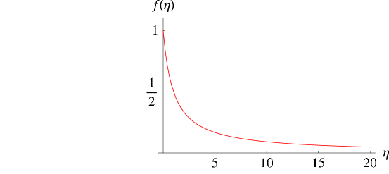
Figure 5.5: The coefficient of the effective potential, $f(\eta)=1/(1+\eta)$, as function of the density of holes in units of $\Lambda$, $\eta=\frac{n}{\Lambda}$.

5.2.6 Summary

In this section, we have presented the complete analytic solution of a previously proposed model [73] of two dimensional Lorentzian quantum gravity including a sum over topologies. The presence of causality constraints imposed on the path-integral histories – physically motivated in [73, 74] – enabled us to derive a new class of continuum theories by taking an unambiguously defined double-scaling limit of a statistical model of simplicially regularized spacetimes. After computing the Laplace transform of the exact one-step propagator of the discrete model, we investigated a two-parameter family, defined by (5.36) and (5.38), of possible scalings for the gravitational (or Newton’s) coupling, from which physical considerations singled out a unique one. For this case, we computed the quantum Hamiltonian, its spectrum and eigenfunctions, as well as the partition function and propagator. Using these continuum results, we then calculated a variety of physical observables, including the average spacetime density of holes and the expectation values of the spatial volume and all its moments.

This should be contrasted with the previous treatment in [73, 74], in which only the one-step partition function with summed-over boundaries was evaluated. Because of the lack of boundary information, no explicit Hamiltonian was obtained there. Moreover, it turns out that the scaling of the couplings which in the current work led to the essentially unique Hamiltonian (5.49) could not have been obtained or even guessed in the previous work. This is simply a consequence of the fact that the dimensionful renormalized boundary cosmological constants make an explicit appearance in the scaling relation (5.48) for $h$, and thus for Newton’s constant. We conclude that – unlike in the case of the original Lorentzian model – for two dimensional causal quantum gravity with topology changes one cannot obtain the correct scalings for the “bulk” coupling constants from the one-step partition function with boundaries summed over (which is easier to compute than the full one-step propagator).

In contrast with what was extrapolated from the single-strip model in [74], the total number of holes in a finite patch of spacetime turns out to be a finite quantity determined by the cosmological and Newton’s constants. Note that this finiteness result has been obtained dynamically and without invoking any fundamental discreteness. Since the density of holes is finite and every hole in the model is infinitesimal, this implies – and is confirmed by explicit calculation – that the expectation value of the number of holes in a general spatial slice of constant time is also infinitesimal. The fact that physically sensible observables are obtained in this toy model reiterates the earlier conclusion [73] that causality-inspired methods can be a useful tool in constructing gravitational path integrals which include a sum over topologies.

From the effective potential displayed in fig. 5.5 one observes that the presence of wormholes in our model leads to a decrease of the “effective” cosmological constant $f(\eta)\Lambda$. In Coleman’s mechanism for driving the cosmological constant $\Lambda$ to zero [76, 77], an additional sum over different baby universes is performed in the path integral, which leads to a distribution of the cosmological constant that is peaked near zero. We do not consider such an additional sum over baby universes, but instead have an explicit expression for the effective potential which shows that an increase in the number of wormholes is accompanied by a decrease of the “effective” cosmological constant. A first step in establishing whether an analogue of our suppression mechanism also exists in higher dimensions would be to try and understand whether one can identify a class of causally preferred topology changes which still leaves the sum over geometries exponentially bounded.

Chapter 6 Conclusions

Despite many attempts, gravity has resiliently resisted a unification with the laws of quantum mechanics. Besides a plethora of technical issues, one is also faced with many interesting conceptual problems. The study of quantum gravity in lower dimensional models ameliorates the technical difficulties while still preserving some of the conceptually fascinating characteristics of quantum gravity.

In this thesis we analyze the very simple model of two dimensional quantum gravity. Although a rather extreme simplification of four dimensional gravity, many of the most fundamental issues are still relevant. Moreover, two dimensional gravity is interesting since it can be viewed as a minimal version of string theory.

The first fundamental aspect where we make a contribution is the problem of topology change of space. Particularly, we present an exactly solvable model which shows that it is possible to incorporate spatial topology changes in the path integral rigorously. We show that if the change in spatial topology is accompanied by a coupling constant it is possible to evaluate the path integral to all orders in the coupling. Furthermore, the model can be viewed as a hybrid between causal and Euclidean dynamical triangulation models. An interesting avenue for further research is the question whether our model has an interpretation within string theory. In particular, is our new coupling constant really equivalent to the string coupling?

The second conceptual topic that we cover is the emergence of geometry from a background independent path integral. We show that from a path integral over noncompact manifolds a classical geometry with constant negative curvature emerges. No initial singularity is present, so the model naturally realizes the Hartle Hawking boundary condition. Furthermore, we demonstrate that under certain conditions the superimposed quantum fluctuations are small! The model is an interesting example where a classical background emerges from background independent quantum gravity in an exactly solvable setting. How does the emergent geometry behave? Can we make contact with effective descriptions of quantum geometry such as noncommutative geometry or doubly special relativity? The answer to these questions is incomplete for now, but the exact solvability of the model suggests that at least a detailed analysis could be possible.

To conclude, we tackle the problem of spacetime topology change. Although we are not able to completely solve the path integral over all manifolds with arbitrary topology, we do obtain some results that indicate that such a path integral might be consistent if suitable causality restrictions are imposed. As a first step we extend the existing formalism of causal dynamical triangulations by a perturbative computation of amplitudes that include manifolds up to genus two. Further we present a toy model where we make the approximation that the holes in the manifold are extremely small. This simplification allows us perform an explicit sum over all genera and analyze the continuum limit exactly. Remarkably, the presence of the infinitesimal wormholes leads to a decrease in the effective cosmological constant, reminiscent of the suppression mechanism considered by Coleman and others in the four-dimensional Euclidean path integral.

The results of this thesis show that we still know very little about the ultimate configuration space of quantum gravity. Even for the extremely simple case of two dimensional quantum gravity various new models can be constructed that seem to lead to a well defined theory of quantum geometry. To understand the situation even better it would be important to have a better continuum understanding of the results of causal dynamical triangulations.

Appendix A Lorentzian triangles

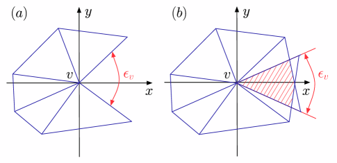
Figure A.1: Illustration of a positive (a) and negative (b) spacelike deficit angle $\epsilon_{v}$ at a vertex $v$.

In this appendix, a brief summary of results on Lorentzian angles is presented, where we follow the treatment and conventions of [13].

Since in CDT one considers simplicial manifolds consisting of Minkowskian triangles, Lorentzian angles or “boosts” naturally appear in the Regge action as rotations around vertices. Recall from Section (2.5.3) that the definition of the scalar curvature at a vertex $v$ is given by (2.25),

$$R_{v}=2\frac{\epsilon_{v}}{V_{v}},$$ (A.1)

where $\epsilon_{v}=2\pi-\sum_{i\supset v}\theta_{i}$ is the deficit angle at a vertex $v$ and $V_{v}$ is the dual volume of the vertex $v$. In general, the spacelike deficit angle $\epsilon_{v}$ can be positive or negative as illustrated in fig. A.1. Furthermore, if the deficit angle is timelike, as shown in fig. A.2, it will be complex. The timelike deficit angles are still additive, but contribute to the curvature (A.1) with the opposite sign. Hence, both spacelike defect and timelike excess increase the curvature, whereas spacelike excess and timelike defect decrease it.

The complex nature of the timelike deficit angles can be seen explicitly by noting that the angles $\theta_{i}$ between two edges $\vec{a}_{i}$ and $\vec{b}_{i}$ (as vectors in Minkowski space) are calculated using

$$\cos\theta_{i}=\frac{\langle\vec{a}_{i},\vec{b}_{i}\rangle}{\langle\vec{a}_{i},\vec{a}_{i}\rangle^{\frac{1}{2}}\langle\vec{b}_{i},\vec{b}_{i}\rangle^{\frac{1}{2}}},\quad\sin\theta_{i}=\frac{\sqrt{\langle\vec{a}_{i},\vec{a}_{i}\rangle\langle\vec{b}_{i},\vec{b}_{i}\rangle-\langle\vec{a}_{i},\vec{b}_{i}\rangle^{2}}}{\langle\vec{a}_{i},\vec{a}_{i}\rangle^{\frac{1}{2}}\langle\vec{b}_{i},\vec{b}_{i}\rangle^{\frac{1}{2}}},$$ (A.2)

where $\langle\cdot,\cdot\rangle$ denotes the flat Minkowskian scalar product and by definition, the square roots of negative arguments are positive imaginary.

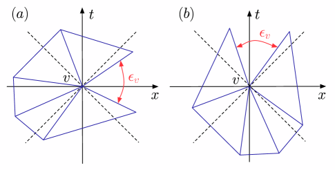
Figure A.2: Illustration of a spacelike (a) and a timelike (b) Lorentzian deficit angle $\epsilon_{v}$ at a vertex $v$.

Having given a concrete meaning to Lorentzian angles, we can now use (A.2) to calculate the volume of Minkowskian triangles which we will then use to explicitly compute the volume terms of the Regge action.

The triangulations we are considering consist of Minkowskian triangles with one spacelike edge of length squared $l_{s}^{2}=a^{2}$ and two timelike edges of length squared $l_{t}^{2}=-\alpha a^{2}$ with $\alpha>0$. The general argument $\alpha>0$ is used to give a mathematically precise prescription of the Wick rotation, but it can be set to $\alpha=1$ after the Wick rotation has been performed. With the use of (A.2) we can calculate the volume of such a Minkowskian triangle, yielding

$$\mathrm{Vol}(\mathrm{triangle})=\frac{a^{2}}{4}\sqrt{4\alpha+1}.$$ (A.3)

Now one can define the Wick rotation $\mathcal{W}$ as the analytic continuation of $\alpha\mapsto-\alpha$ through the lower-half plane. One then sees that for $\alpha>\frac{1}{2}$ under this prescription $i\,\mathrm{Vol}(\mathrm{triangle})\mapsto-\mathrm{Vol}(\mathrm{triangle})$ (up to a $\mathcal{O}(1)$ constant which can be absorbed in the corresponding coupling constant in the action). This ensures that

$$\mathcal{W}:\quad e^{i\,S_{\mathrm{Regge}}(T^{lor})}\mapsto e^{-\,S_{\mathrm{Regge}}(T^{eu})},\quad\alpha>\frac{1}{2}.$$ (A.4)

In the following we set $\alpha=1$ again. Generalizations of this treatment to dimension $d=3,4$ can be found in [80].

Appendix B Alternative scalings

In this appendix we discuss the scalings with $\beta=1$ which we discarded as unphysical in Sec. (5.2.4) above. We proceed as before by inserting the scaling relations (5.34) and (5.46) into the composition law (5.40). Instead of using $\beta=\frac{3}{2}$ we set $\beta=1$, leading to the scaling

$$h=\frac{1}{4}\,h_{ren}\,a\,\sqrt{\Lambda}^{\alpha}(X+Y)^{1-\alpha},$$ (B.1)

where the normalization factor on the right-hand side has been chosen for later convenience. Up to first order in $a$ one obtains

$$(1-a\hat{H}+\mathcal{O}(a^{2}))\psi(X)=\int^{i\infty}_{-i\infty}\frac{dZ}{2\pi i}\left\{A(X,Z)+B(X,Z)a+\mathcal{O}(a^{2})\right\}\psi(Z),$$ (B.2)

where the leading-order contribution is given by

$$A(X,Z)=\frac{2}{(Z-X)\left(1+C(X,Z)\right)}$$ (B.3)

with

$$C(X,Z)=\sqrt{1-h_{ren}^{2}(X-Z)^{-2\alpha}\Lambda^{\alpha}}.$$ (B.4)

For the Laplace transform of $A(X,Z)$ to yield a delta-function, the scaling should be chosen such that $\alpha\leqslant 0$. Considering now the terms of first order in $a$,

$$B(X,Z) = \frac{h_{ren}^{2}(X+Z-4Z\gamma)\Lambda^{\alpha}}{(X-Z)^{1+2\alpha}C(X,Z)\left(1+C(X,Z)\right)^{2}}$$ (B.5)

$$- 2\,\frac{XZ-2\Lambda+\gamma(X-Z)^{2}}{(X-Z)^{2}C(X,Z)\left(1+C(X,Z)\right)},$$

one finds that for $\alpha\leqslant-1$ the continuum limit is independent of any “hole contribution” (i.e. terms depending on $h_{ren}$) and therefore leads to the usual Lorentzian model. This becomes clear when one expands the last term of (B.5) in $(X-Z)$, resulting in

$$\frac{XZ-2\Lambda}{(X-Z)^{2}C\left(1+C\right)}=\frac{1}{2}\frac{XZ-2\Lambda}{(X-Z)^{2}}\left(1+\frac{3}{4}\,h_{ren}^{2}\Lambda^{\alpha}(X-Z)^{-2\alpha}+\mathcal{O}((X-Z)^{-4\alpha})\right).$$ (B.6)

For $\alpha\leqslant-1$ the term depending on $h_{ren}$ does not have a pole and therefore does not contribute to the Hamiltonian. Since we are only interested in non-fractional poles, this leaves as possible $\alpha$-values only $\alpha=0$ and $\alpha=-\frac{1}{2}$.

B.1 The case $\beta=1$, $\alpha=0$

For $\alpha=0$ the Hamiltonian retains a $\gamma$-dependence contained in the first line of (B.5). Since there is no immediate physical interpretation of $\gamma$ in our model, it seems natural to choose $\gamma=0$, although strictly speaking this does not resolve the problem of explaining the $\gamma$-dependence of the continuum limit. Setting this question aside, one may simply look at the resulting model as an interesting integrable model in its own right. In order to obtain a delta-function to leading order, one still needs to normalize the transfer matrix by a constant factor $2/(1+s)$, with $s:=\sqrt{1-h_{ren}^{2}}$. After setting $\gamma=0$ and performing an inverse Laplace transformation, the Hamiltonian reads

$$\hat{H}(L,\frac{\partial}{\partial L})=\frac{1}{s}\left(-L\frac{\partial^{2}}{\partial L^{2}}-s\frac{\partial}{\partial L}+2\Lambda L\right).$$ (B.7)

It is self-adjoint with respect to the measure $d\mu(L)=L^{s-1}dL$. Further setting $L=\frac{\varphi^{2}}{2\,s}$ one encounters the one-dimensional Calogero Hamiltonian

$$\hat{H}(\varphi,\frac{\partial}{\partial\varphi})=-\frac{1}{2}\frac{\partial^{2}}{\partial\varphi^{2}}+\frac{1}{2}\omega^{2}\varphi^{2}-\frac{1}{8}\frac{A}{\varphi^{2}},$$ (B.8)

with $\omega\!=\!\frac{\sqrt{2\Lambda}}{s}$ and $A\!=\!1-4(1-s)^{2}$, which implies that the model covers the parameter range $-3\leqslant A\leqslant 1$. The maximal range for which the Calogero Hamiltonian is self-adjoint is $-\infty<A\leqslant 1$. The usual Lorentzian model without holes corresponds to $A\!=\!1$. The Hamiltonian ((B.8)) has already appeared in a causal dynamically triangulated model where the two dimensional geometries were decorated with a certain type of “outgrowth” or small “baby universes” [78]. This model covered the parameter range $0\leqslant A\leqslant 1$.

The eigenvectors of the Hamiltonian ((B.7)) are given by

$$\psi_{n}(L)=\mathcal{A}_{n}e^{-\sqrt{2\Lambda}L}\,{}_{1}F_{1}(-n,s,2\sqrt{2\Lambda}L),\quad d\mu(L)=L^{s-1}dL,$$ (B.9)

where ${}_{1}F_{1}(-n,a,b)$ is the Kummer confluent hypergeometric function. The eigenvectors form an orthonormal basis with the normalization factors

$$\mathcal{A}_{n}=(8\Lambda)^{\frac{s}{4}}\sqrt{\frac{\Gamma(n+s)}{\Gamma(n+1)\Gamma(s)^{2}}}$$ (B.10)

and the corresponding eigenvalues

$$E_{n}=\frac{\sqrt{2\Lambda}}{s}(2n+s),\quad n=0,1,2,...\,.$$ (B.11)

One sees explicitly that the case $s\!=\!1$ or, equivalently, $A\!=\!1$ corresponds to the pure two dimensional CDT model.

B.2 The case $\beta=1$, $\alpha=-\frac{1}{2}$

For $\alpha=-\frac{1}{2}$ the result does not depend on $\gamma$ and therefore on the detailed manner in which we approach the critical point. However, the Hamiltonian

$$\hat{H}(L,\frac{\partial}{\partial L})=-L\frac{\partial^{2}}{\partial L^{2}}-\frac{\partial}{\partial L}+2\,\Lambda\,L-\frac{3}{4}\,h_{ren}^{2}\Lambda^{-1/2}\,\frac{\partial^{2}}{\partial L^{2}}$$ (B.12)

cannot be made self-adjoint with respect to any measure $d\mu(L)$ because the boundary part of the partial integration always gives a nonvanishing contribution. We therefore discard this possibility.

Appendix C The density of holes of an infinitesimal strip

In this appendix we give an alternative derivation of the spacetime density $n$ of holes and explicitly show that the number of holes in a spacetime strip of infinitesimal time duration $a$ is also infinitesimal. The operator in the $L$-representation of the number of holes per infinitesimal strip with fixed initial boundary $L$ can be calculated by

$$\hat{N}_{{\mathfrak{g}},a\rightarrow 0}=\hat{T}^{-1}\frac{h_{ren}}{2}\frac{\partial\,\hat{T}}{\partial h_{ren}},$$ (C.1)

where $\hat{T}$ is the transfer matrix defined in (5.21). Using $\hat{T}=1-a\hat{H}+\mathcal{O}(a^{2})$ and evaluating (C.1) to leading order in $a$ gives

$$\hat{N}_{{\mathfrak{g}},a\rightarrow 0}=-a\,\frac{h_{ren}}{2}\frac{\partial\hat{H}}{\partial h_{ren}}+\mathcal{O}(a^{2})=2\,\Lambda\,h_{ren}^{2}\,L\,a+\mathcal{O}(a^{2}).$$ (C.2)

Similarly, the volume operator of the same infinitesimal spacetime strip in the $L$-representation is given by

$$\hat{V}_{a\rightarrow 0}=-\hat{T}^{-1}\frac{\partial\,\hat{T}}{\partial\Lambda}=a\,\frac{\partial\hat{H}}{\partial\Lambda}+\mathcal{O}(a^{2})=2\,(1-h_{ren}^{2})\,L\,a+\mathcal{O}(a^{2}).$$ (C.3)

Although both expressions (C.2) and (C.3) vanish in the limit as $a\rightarrow 0$ (and therefore the number of holes and the strip volume are both “infinitesimal”), their quotient evaluates to a finite number independent of $L$, namely,

$$n=\frac{N_{{\mathfrak{g}},a\rightarrow 0}}{V_{a\rightarrow 0}}=\frac{h_{ren}^{2}}{1-h_{ren}^{2}}\,\Lambda.$$ (C.4)

This is the exactly the same result for the spacetime density $n$ of holes as we obtained earlier from the continuum partition function (5.63).

References

- [1] J. Ambjorn, R. Loll, Y. Watabiki, W. Westra, and S. Zohren, “A String Field Theory based on Causal Dynamical Triangulations,” JHEP 05 (2008) 032, 0802.0719.
- [2] J. Ambjorn, R. Loll, Y. Watabiki, W. Westra, and S. Zohren, “A Matrix Model for 2D Quantum Gravity defined by Causal Dynamical Triangulations,” Phys. Lett. B665 (2008) 252–256, 0804.0252.
- [3] S. Carlip, “Quantum gravity in 2+1 dimensions,”. Cambridge, UK: Univ. Pr. (1998) 276 p.
- [4] M. Banados, C. Teitelboim, and J. Zanelli, “The black hole in three-dimensional space-time,” Phys. Rev. Lett. 69 (1992) 1849–1851, hep-th/9204099.
- [5] E. Witten, “Three-dimensional gravity revisited,” arXiv:0706.3359.
- [6] E. Witten, “(2+1) -dimensional gravity as an exactly soluble system,” Nucl. Phys. B311 (1988) 46.
- [7] A. M. Polyakov, “Quantum geometry of bosonic strings,” Phys. Lett. B103 (1981) 207–210.
- [8] A. M. Polyakov, “Gauge fields and strings,”. Chur, Switzerland: harwood (1987) 301 p. (contemporary concepts in physics, 3).
- [9] A. M. Polyakov, “Quantum gravity in two-dimensions,” Mod. Phys. Lett. A2 (1987) 893.
- [10] E. J. Martinec, “The annular report on non-critical string theory,” hep-th/0305148.
- [11] S. W. Hawking, “The path integral approach to quantum gravity,”. In Hawking, S.W., Israel, W.: General Relativity, 746- 789.
- [12] T. Regge, “General relativity without coordinates,” Nuovo Cim. 19 (1961) 558–571.
- [13] R. Sorkin, “Time evolution problem in Regge calculus,” Phys. Rev. D12 (1975) 385–396.
- [14] M. Rocek and R. M. Williams, “Quantum Regge calculus,” Phys. Lett. B104 (1981) 31.
- [15] J. Ambjorn, B. Durhuus, and T. Jonsson, “Quantum geometry. a statistical field theory approach,” Cambridge Monogr. Math. Phys. 1 (1997) 1–363.
- [16] G. ’t Hooft, “A planar diagram theory for strong interactions,” Nucl. Phys. B72 (1974) 461.
- [17] P. H. Ginsparg and G. W. Moore, “Lectures on 2-d gravity and 2-d string theory,” hep-th/9304011.
- [18] P. DiFrancesco, P. H. Ginsparg, and J. Zinn-Justin, “2-d gravity and random matrices,” Phys. Rept. 254 (1995) 1–133, hep-th/9306153.
- [19] V. Fateev, A. B. Zamolodchikov, and A. B. Zamolodchikov, “Boundary Liouville field theory. i: Boundary state and boundary two-point function,” hep-th/0001012.
- [20] A. B. Zamolodchikov and A. B. Zamolodchikov, “Liouville field theory on a pseudosphere,” hep-th/0101152.
- [21] J. Ambjorn and R. Loll, “Non-perturbative Lorentzian quantum gravity, causality and topology change,” Nucl. Phys. B536 (1998) 407–434, hep-th/9805108.
- [22] C. Teitelboim, “Causality versus gauge invariance in quantum gravity and supergravity,” Phys. Rev. Lett. 50 (1983) 705.
- [23] C. Teitelboim, “The proper time gauge in quantum theory of gravitation,” Phys. Rev. D28 (1983) 297.
- [24] J. Ambjorn, J. Jurkiewicz, and R. Loll, “Emergence of a 4d world from causal quantum gravity,” Phys. Rev. Lett. 93 (2004) 131301, hep-th/0404156.
- [25] J. Ambjorn, J. Jurkiewicz, and R. Loll, “Semiclassical universe from first principles,” Phys. Lett. B607 (2005) 205–213, hep-th/0411152.
- [26] J. Ambjorn, J. Jurkiewicz, and R. Loll, “Spectral dimension of the universe,” Phys. Rev. Lett. 95 (2005) 171301, hep-th/0505113.
- [27] J. Ambjorn, J. Jurkiewicz, and R. Loll, “Reconstructing the universe,” Phys. Rev. D72 (2005) 064014, hep-th/0505154.
- [28] J. Ambjorn, J. Jurkiewicz, and R. Loll, “The universe from scratch,” Contemp. Phys. 47 (2006) 103–117, hep-th/0509010.
- [29] J. Ambjorn, J. Jurkiewicz, and R. Loll, “Quantum gravity, or the art of building spacetime,” hep-th/0604212.
- [30] R. Nakayama, “2-D quantum gravity in the proper time gauge,” Phys. Lett. B325 (1994) 347–353, hep-th/9312158.
- [31] J. Ambjorn, J. Correia, C. Kristjansen, and R. Loll, “On the relation between Euclidean and Lorentzian 2d quantum gravity,” Phys. Lett. B475 (2000) 24–32, hep-th/9912267.
- [32] D. Oriti, “The group field theory approach to quantum gravity,” gr-qc/0607032.
- [33] L. Bombelli, J.-H. Lee, D. Meyer, and R. Sorkin, “Space-time as a causal set,” Phys. Rev. Lett. 59 (1987) 521.
- [34] S. Holst, “Barbero’s Hamiltonian derived from a generalized Hilbert-Palatini action,” Phys. Rev. D53 (1996) 5966–5969, gr-qc/9511026.
- [35] G. W. Gibbons and S. W. Hawking, “Action integrals and partition functions in quantum gravity,” Phys. Rev. D15 (1977) 2752–2756.
- [36] J. Ambjorn, R. Loll, J. L. Nielsen, and J. Rolf, “Euclidean and Lorentzian quantum gravity: Lessons from two dimensions,” Chaos Solitons Fractals 10 (1999) 177–195, hep-th/9806241.
- [37] H. Kawai, N. Kawamoto, T. Mogami, and Y. Watabiki, “Transfer matrix formalism for two-dimensional quantum gravity and fractal structures of space-time,” Phys. Lett. B306 (1993) 19–26, hep-th/9302133.
- [38] S. S. Gubser and I. R. Klebanov, “Scaling functions for baby universes in two-dimensional quantum gravity,” Nucl. Phys. B416 (1994) 827–849, hep-th/9310098.
- [39] H. Aoki, H. Kawai, J. Nishimura, and A. Tsuchiya, “Operator product expansion in two-dimensional quantum gravity,” Nucl. Phys. B474 (1996) 512–528, hep-th/9511117.
- [40] J. Cheeger, W. Muller, and R. Schrader, “On the curvature of piecewise flat spaces,” Commun. Math. Phys. 92 (1984) 405.
- [41] H. W. Hamber and R. M. Williams, “Higher derivative quantum gravity on a simplicial lattice,” Nucl. Phys. B248 (1984) 392.
- [42] J. Ambjorn, J. L. Nielsen, J. Rolf, and G. K. Savvidy, “Spikes in quantum Regge calculus,” Class. Quant. Grav. 14 (1997) 3225–3241, gr-qc/9704079.
- [43] P. Menotti and P. P. Peirano, “Functional integration for Regge gravity,” Nucl. Phys. Proc. Suppl. 57 (1997) 82–90, gr-qc/9702020.
- [44] J. Ambjorn, B. Durhuus, and J. Frohlich, “Diseases of triangulated random surface models, and possible cures,” Nucl. Phys. B257 (1985) 433.
- [45] F. David, “Planar diagrams, two-dimensional lattice gravity and surface models,” Nucl. Phys. B257 (1985) 45.
- [46] V. A. Kazakov, A. A. Migdal, and I. K. Kostov, “Critical properties of randomly triangulated planar random surfaces,” Phys. Lett. B157 (1985) 295–300.
- [47] J. Ambjørn, L. Chekhov, C. F. Kristjansen, and Y. Makeenko, “Matrix model calculations beyond the spherical limit,” Nucl. Phys. B404 (1993) 127–172, hep-th/9302014.
- [48] B. Eynard, “Topological expansion for the 1-hermitian matrix model correlation functions,” JHEP 11 (2004) 031, hep-th/0407261.
- [49] J. Ambjorn and S. Varsted, “Three-dimensional simplicial quantum gravity,” Nucl. Phys. B373 (1992) 557–580.
- [50] M. E. Agishtein and A. A. Migdal, “Three-dimensional quantum gravity as dynamical triangulation,” Mod. Phys. Lett. A6 (1991) 1863–1884.
- [51] J. Ambjorn and J. Jurkiewicz, “Four-dimensional simplicial quantum gravity,” Phys. Lett. B278 (1992) 42–50.
- [52] M. E. Agishtein and A. A. Migdal, “Critical behavior of dynamically triangulated quantum gravity in four-dimensions,” Nucl. Phys. B385 (1992) 395–412, hep-lat/9204004.
- [53] P. Bialas, Z. Burda, A. Krzywicki, and B. Petersson, “Focusing on the fixed point of 4d simplicial gravity,” Nucl. Phys. B472 (1996) 293–308, hep-lat/9601024.
- [54] S. Catterall, R. Renken, and J. B. Kogut, “Singular structure in 4d simplicial gravity,” Phys. Lett. B416 (1998) 274–280, hep-lat/9709007.
- [55] P. Di Francesco, E. Guitter, and C. Kristjansen, “Integrable 2d Lorentzian gravity and random walks,” Nucl. Phys. B567 (2000) 515–553, hep-th/9907084.
- [56] G. T. Horowitz, “Topology change in classical and quantum gravity,” Class. Quant. Grav. 8 (1991) 587–602.
- [57] F. Dowker, “Topology change in quantum gravity,” gr-qc/0206020.
- [58] J. Ambjorn, J. Jurkiewicz, and R. Loll, “Lorentzian and Euclidean quantum gravity: Analytical and numerical results,” hep-th/0001124.
- [59] J. Ambjorn, R. Loll, W. Westra, and S. Zohren, “Putting a cap on causality violations in CDT,” JHEP 12 (2007) 017, 0709.2784.
- [60] N. Ishibashi and H. Kawai, “String field theory of noncritical strings,” Phys. Lett. B322 (1994) 67–78, hep-th/9312047.
- [61] Y. Watabiki, “Construction of noncritical string field theory by transfer matrix formalism in dynamical triangulation,” Nucl. Phys. B441 (1995) 119–166, hep-th/9401096.
- [62] S. Jain and S. D. Mathur, “World sheet geometry and baby universes in 2-d quantum gravity,” Phys. Lett. B286 (1992) 239–246, hep-th/9204017.
- [63] J. Louko and R. D. Sorkin, “Complex actions in two-dimensional topology change,” Class. Quant. Grav. 14 (1997) 179–204, gr-qc/9511023.
- [64] J. Ambjorn, R. Janik, W. Westra, and S. Zohren, “The emergence of background geometry from quantum fluctuations,” Phys. Lett. B641 (2006) 94–98, gr-qc/0607013.
- [65] N. Seiberg and D. Shih, “Branes, rings and matrix models in minimal (super) string theory,” JHEP 02 (2004) 021, hep-th/0312170.
- [66] J. Ambjorn, S. Arianos, J. A. Gesser, and S. Kawamoto, “The geometry of ZZ-branes,” Phys. Lett. B599 (2004) 306–312, hep-th/0406108.
- [67] J. Ambjorn and J. A. Gesser, “World-sheet dynamics of ZZ branes,” arXiv:0706.3231 [hep-th].
- [68] J. B. Hartle and S. W. Hawking, “Wave function of the universe,” Phys. Rev. D28 (1983) 2960–2975.
- [69] B. Durhuus, J. Frohlich, and T. Jonsson, “Critical behavior in a model of planar random surfaces,” Nucl. Phys. B240 (1984) 453.
- [70] J. Ambjorn and B. Durhuus, “Regularized bosonic strings need extrinsic curvature,” Phys. Lett. B188 (1987) 253.
- [71] J. Ambjorn, B. Durhuus, and T. Jonsson, “Summing over all genera for : a toy model,” Phys. Lett. B244 (1990) 403–412.
- [72] R. Loll, W. Westra, and S. Zohren, “Taming the cosmological constant in 2d causal quantum gravity with topology change,” Nucl. Phys. B751 (2006) 419–435, hep-th/0507012.
- [73] R. Loll and W. Westra, “Sum over topologies and double-scaling limit in 2d Lorentzian quantum gravity,” Class. Quant. Grav. 23 (2006) 465–472, hep-th/0306183.
- [74] R. Loll and W. Westra, “Space-time foam in 2d and the sum over topologies,” Acta Phys. Polon. B34 (2003) 4997–5008, hep-th/0309012.
- [75] R. Loll, “A discrete history of the Lorentzian path integral,” Lect. Notes Phys. 631 (2003) 137–171, hep-th/0212340.
- [76] S. R. Coleman, “Why there is nothing rather than something: a theory of the cosmological constant,” Nucl. Phys. B310 (1988) 643.
- [77] I. R. Klebanov, L. Susskind, and T. Banks, “Wormholes and the cosmological constant,” Nucl. Phys. B317 (1989) 665–692.
- [78] P. Di Francesco, E. Guitter, and C. Kristjansen, “Generalized Lorentzian gravity in (1+1) d and the Calogero Hamiltonian,” Nucl. Phys. B608 (2001) 485–526, hep-th/0010259.
- [79] B. Durhuus and C. W. H. Lee, “A string bit Hamiltonian approach to two-dimensional quantum gravity,” Nucl. Phys. B623 (2002) 201–219, hep-th/0108149.
- [80] J. Ambjorn, J. Jurkiewicz, and R. Loll, “Dynamically triangulating Lorentzian quantum gravity,” Nucl. Phys. B610 (2001) 347–382, hep-th/0105267.
- [81] A. Prudnikov, Y. Brychkov, and O. Marichev, “Integrals and series: vol. 2: Special functions,”. New York: Gordon and Breach (1986).
- [82] J. Ambjorn, J. Jurkiewicz, and R. Loll, “A non-perturbative Lorentzian path integral for gravity,” Phys. Rev. Lett. 85 (2000) 924–927, hep-th/0002050.