Transport and bistable kinetics of a Brownian particle in a nonequilibrium environment

Abstract

A system reservoir model, where the associated reservoir is modulated by an external colored random force, is proposed to study the transport of an overdamped Brownian particle in a periodic potential. We then derive the analytical expression for the average velocity, mobility, and diffusion rate. The bistable kinetics and escape rate from a metastable state in the overdamped region are studied consequently. By numerical simulation we then demonstrate that our analytical escape rate is in good agreement with that of numerical result.

I Introduction

As an immediate consequence of stochastic dynamics, it is observed that thermal diffusion in a periodic potential plays a prominent role in various cases such as Josephson’s junction refja , diffusion in crystal surface refjb , noise limit cycle oscillators refjc etc. There has been a renewed interest in recent times in the study of transport properties of Brownian particles moving in a periodic potential refjd with special emphasis on coherent transport and giant diffusion refje . These studies have been motivated in part by an attempt to understand the mechanism of movement of protein motors in biological systems refjf . Several physical models have been proposed to understand the transport phenomena in such systems such as vibrational ratchet refjg , rocking ratchet refjh , diffusion ratchet refji ; refjj , correlation ratchet refjk , etc. Such ratchet models have a wide range of application in biology and nanoscopic systems refjl , because of their extraordinary success in exploring experimental observations on biochemical molecular motors, active in muscle contraction refjm , observation of directed transport in photovoltaic and photoreflective materials refjn , etc. In all the above models, the potential is taken to be asymmetric in space. One can also obtain a unidirectional current in the presence of spatially symmetric potential. For such non-equilibrium systems, one requires time asymmetric random force refjo or space dependent diffusion refjp ; refjq ; refjr . In passing, we want to mention the fact that to explain the role of Levy stable noise in transport phenomena in presence of bistable, metastable, and periodic potentials with broken symmetry, several elegant approaches have been suggested recently pre .

Traditionally, Langevin equation describing the dynamics of a Brownian particle coupled to a thermal reservoir is a tool for modeling several aspects of nonequilibrium phenomena lax . In addition to the Langevin dynamics, one often takes into account the probabilistic aspect of the random dynamics through the usage of Fokker-Planck equation risken . Both of the approaches utilize the relation between the random fluctuations imposed by the reservoir into the Brownian particle and the relaxation of the imposed energy back to the reservoir, through the fluctuation-dissipation relation (FDR) kubo . FDR takes into account the balance between the energy input (to the system from the reservoir) and output (from the system into the reservoir) through the detailed balance mechanism. Typical signature of such a system is the attainment of equilibrium in the asymptotic limit.

An additional external random driving applied to the Brownian particle can break this balance mechanism and make the composite system open lw , the direct consequence of which is the loss of FDR. In addition to that, the system hardly reaches the equilibrium state in the long time limit but rather attains a stationary steady state lw . However, a driving of the reservoir by an external random field bravo creates a thermodynamic consistency condition analogous to FDR jrcpre1 that leads to the study of several interesting phenomena jrcpre1 ; jrcpre2 ; jrcpre3 ; jrcjpa ; jrcjcp in chemical physics. The net effect of the reservoir driving by an external random force is the creation of an effective temperature in addition to the thermal energy $k_{B}T$ exerted by the reservoir on the system of interest. As shown recently, this effective temperature can enhance the reaction rate in condensed media jrcpre1 ; jrcpre2 ; jrcpre3 as well as generate directed motion in a periodic system jrcjpa ; jrcjcp .

In the present paper, we consider a system-reservoir model where the bath is modulated by an external noise. However, when the reservoir is modulated by an external noise it is likely that it induces fluctuations in the polarization of the reservoir due to the external noise from a microscopic point of view and one may expect that the non-equilibrium situation created by modulating the bath makes its presence felt in the transport property and also in the kinetics of the Brownian particle. A number of different situations depicting the modulation of the bath may be physically relevant. For an example, we may consider the case of a Brownian particle when the response of the solvent is time-dependent, as in a liquid crystal, or in the reaction-diffusion mechanism in super-critical lattice, or the growth in living polymerization refjrr .

To observe the effects of external stochastic modulation one can carry out the experiment in a photochemically active solvent (the heat bath) where the solvent is under the influence of external monochromatic light with fluctuating intensity which is absorbed solely by the solvent molecules. As a result of this, the modulated solvent heats up due to the conversion of light energy into heat energy by radiation less relaxation process, and an effective temperature-like quantity develops due to constant input of energy. Since the fluctuations in light intensity result in the polarization of the solvent molecules the effective reaction field around the reactant gets modified refjss . Our theoretical model can be tested experimentally to study the directional motion and mean first passage time of artificial chemical rotors in photovoltaic solvent refjs .

There are some precedents for our model that are worth mentioning. Bravo et al. bravo dealt with a related problem: a classical system in a heat bath with an additive external noise. In the quantum case, Faid and Fox refjtt proposed a stochastic coupling between the system and a heat bath as a phenomenological mechanism of relaxation for the bath. Mañas et al. refju considered the problem of a system coupled to an ensemble of independent harmonic oscillators as a reservoir. We have also considered the dynamics of a metastable state non-linearly coupled to a heat bath driven by an external noise to study the escape rate from a metastable state jrcpre3 . In the present work, we address the so-called ratchet problem and bistable kinetics of a Brownian particle for a thermodynamically open system where the associated bath is modulated by a colored noise and we explore the dependence of various parameters of the external noise on the transport phenomena and bistable kinetics.

To get insight of situations encountered in the growing number of nano and microscale experiments, our model can be used as a potential tool. For instance, several DNA nanomotors have been recently suggested epl ; epl8 . These machines are relatively slow and do not perform continuous rotation. Very recently, a rotary DNA nanomachine that shows a continuous rotation has been proposed epl . This motor consists of a DNA ring whose elastic features are tuned such that it can be externally driven by a periodic temperature change. Our model proposed in this paper can be used as a theoretical avenue to examine the periodic temperature change via a physically motivated microscopic Hamiltonian picture. Optical tweezers t1 , which is capable of manipulating nanometer and micrometer sized dielectric particles by exerting extremely small forces via a highly focused laser beam, is often used to manipulate and study single molecules by interacting with a bead that has been attached to that molecule. DNA and the proteins and enzymes that interact with it are commonly studied in this way. At this juncture, we want to mention the fact that our development present in this article can be used as a theoretical model to understand the phenomena of heating of the liquid surrounding a bead in an optical tweezers setup t13 .

The organization of the paper is as follows: In Sec. II, starting from a microscopic Hamiltonian picture of a system linearly coupled with a harmonic reservoir which is modulated by a noise with arbitrary decaying memory kernel, we have derived the Langevin equation with an effective noise $\eta(t)$ and then explored its statistical property. Employing the functional calculus method lw ; refjw ; refjy , we then obtain the Fokker-Planck-Smoluchowski equation in Sec. III, corresponding to the Langevin equation valid in the over damped limit and for rapid fluctuations whose correlation function vanishes rapidly. In Sec. IV, we have calculated the steady current in a ratchet potential and derived the expression for diffusion rate and mobility. As another application of our development, we study the bistable kinetics to obtain the stationary probability density function (PDF) and the barrier crossing rate. The summarizing remarks are presented in Sec. VI preceded by a numerical application in Sec. V.

II The Model: Heat bath modulated by external noise

We consider a classical particle of unit mass coupled to a heat bath consisting of a set of $N$-numbers of mass weighted harmonic oscillators with frequency $\{\omega_{j}\}$. The heat-bath is externally driven by a Gaussian random force $\epsilon(t)$ with an arbitrary decaying correlation function. The total Hamiltonian of such a composite system can be written as zwanzig ; jrcpre1

$$H=\frac{v^{2}}{2}+V({x})+\sum_{j=1}^{N}\left[\frac{{v}_{j}^{2}}{2}+\frac{1}{2}\omega_{j}^{2}(x_{j}-c_{j}x)^{2}\right]+H_{\rm int}.$$ (1)

In the above equation $x$ and $v$ are the coordinate and the velocity of the system particle, respectively, and $V(x)$ is the potential energy of the system. $\{x_{j},v_{j}\}$ are the variables for the $j$th oscillator with characteristic frequency $\omega_{j}$. The system particle is coupled to the bath oscillator linearly through the general coupling terms $c_{j}\omega_{j}x$ where $c_{j}$ is the coupling strength for the system-bath interaction. The interaction between the heat bath and the external noise is represented by the term $H_{\rm int}$ which we take as jrcpre1 ; landau

$$H_{\rm int}=\sum_{j=1}^{N}\kappa_{j}x_{j}\epsilon(t),$$ (2)

where $\kappa_{j}$ denotes the coupling strength of interaction and $\epsilon(t)$ is an external noise which is assumed to be stationary, Gaussian with zero mean and arbitrary decaying correlation function, the statistical property of which is given by

$$\langle\epsilon(t)\rangle_{e}=0,\langle\epsilon(t)\epsilon(t^{\prime})\rangle_{e}=2D_{e}\Psi(t-t^{\prime}),$$ (3)

where $D_{e}$ is the external noise strength and $\Psi(t)$ is the external noise memory kernel which is assumed to be a decaying function of its argument and $\langle\cdots\rangle_{e}$ implies averaging over each realization of $\epsilon(t)$. Eliminating the bath degrees of freedom in the usual way zwanzig ; jrcpre1 , we get the Langevin equation for the system particle

$$\dot{x} = {v},$$

$$\dot{v} = -V^{\prime}({x})-\int_{0}^{t}dt^{\prime}\gamma(t-t^{\prime})v(t^{\prime})+f(t)+\pi(t),$$ (4)

where the memory kernel $\gamma(t)$ and the Langevin force term $f(t)$ are given, respectively, by

$$\gamma(t) = \sum_{j=1}^{N}c_{j}^{2}\omega_{j}^{2}\cos(\omega_{j}t),$$ (5)

$$f(t) = \sum_{j=1}^{N}c_{j}\omega_{j}^{2}\left\{[x_{j}(0)-c_{j}x(0)]\cos(\omega_{j}t)\right.$$ (6)

$$\left.+\frac{v_{j}(0)}{\omega_{j}}\sin(\omega_{j}t)\right\}.$$

In Eq.(II), $\pi(t)$ is the fluctuating force generated due to the external stochastic forcing of the bath by $\epsilon(t)$ and is given by

$$\pi(t)=-\int_{0}^{t}dt^{\prime}\varphi(t-t^{\prime})\epsilon(t^{\prime}),$$ (7)

with

$$\varphi(t)=\sum_{j=1}^{N}c_{j}\omega_{j}\kappa_{j}\sin(\omega_{j}t).$$ (8)

The form of Eq.(II) reveals that the system is driven by two fluctuating forces, $f(t)$ and $\pi(t)$. $\pi(t)$ is a dressed noise originating due to the bath modulation by external noise $\epsilon(t)$, and $f(t)$ is the thermal noise due to system-bath coupling. To define the statistical properties of $f(t)$, we assume that the initial distribution is such that the bath is equilibrated at $t=0$ in the presence of the system but in the absence of the external noise $\epsilon(t)$ such that

$$\langle f(t)\rangle=0,\langle f(t)f(t^{\prime})\rangle=k_{B}T\gamma(t-t^{\prime}),$$ (9)

where $k_{B}$ is the Boltzmann constant and $T$ is the equilibrium temperature, $\langle\cdots\rangle$ implies the usual average over the initial distribution which is assumed to be a canonical distribution of Gaussian form zwanzig ; jrcpre1

$$\mathbb{P}=\mathcal{N}\exp\left\{-\frac{v_{j}^{2}(0)+\omega_{j}^{2}(x_{j}(0)-c_{j}x(0))^{2}}{2k_{B}T}\right\},$$

where $\mathcal{N}$ is the normalization constant. Now at $t=0_{+}$, the external noise agency is switched on to modulate the bath. Here, we define an effective Gaussian noise $\eta(t)=f(t)+\pi(t)$ the statistical property of which can be described by

$$\langle\langle\eta(t)\rangle\rangle = 0,$$

$$\langle\langle\eta(t)\eta(t^{\prime})\rangle\rangle = k_{B}T\gamma(t-t^{\prime})+2D_{e}\int_{0}^{t}dt^{\prime\prime}\int_{0}^{t^{\prime}}dt^{\prime\prime\prime}$$

$$\times\varphi(t-t^{\prime\prime})\varphi(t^{\prime}-t^{\prime\prime\prime})\Psi(t^{\prime\prime}-t^{\prime\prime\prime}),$$

$$= G(t-t^{\prime})\text{ (say)}.$$

In Eq.(II), $\langle\langle\cdots\rangle\rangle$ means that we have taken two averages independently, average over initial distribution of bath variables and average over each realization of $\epsilon(t)$. While deriving Eq.(II), we have made the assumption $\langle\langle\eta(t)\eta(t^{\prime})\rangle\rangle=G(t-t^{\prime})$, which can not be proved unless the structure of $\varphi(t)$ is explicitly given. As we shall see later it is a valid assumption for a particular choice of coupling coefficients and for external stationary noise processes. It should be realized that Eq.(II) is not a fluctuation-dissipation relation (FDR) due to the appearance of the external noise intensity, rather it serves as a thermodynamic consistency relation.

To obtain a finite result in the continuum limit, i.e., for $N\rightarrow\infty$, the coupling function $c_{i}=c(\omega)$ and $\kappa_{i}=\kappa(\omega)$ are chosen as $c(\omega)=c_{0}/\omega\sqrt{\tau_{c}}$ and $\kappa(\omega)=\kappa_{0}\omega\sqrt{\tau_{c}}$. Consequently, $\gamma(t)$ and $\varphi(t)$ reduce to

$$\gamma(t)=\frac{c_{0}^{2}}{\tau_{c}}\int d\omega\rho(\omega)\cos\omega t,$$ (11)

and

$$\varphi(t)=c_{0}\kappa_{0}\int d\omega\rho(\omega)\omega\sin\omega t,$$ (12)

where $c_{0}$ and $\kappa_{0}$ are constants and $\tau_{c}$ is the correlation time of the heat bath. For $\tau_{c}\rightarrow 0$ we obtain a $\delta$-correlated noise process. $1/\tau_{c}$ may be characterized as the cut off frequency of the bath oscillators. $\rho(\omega)$ is the density of modes of the heat bath which is assumed to be Lorentzian

$$\rho(\omega)=\frac{2\tau_{c}}{\pi(1+\omega^{2}\tau_{c}^{2})}.$$ (13)

The above assumption resembles broadly the behavior of the hydrodynamical modes refjz ; refjzz in a microscopic system and is frequently used by the chemical physics community refjz . With these forms of $\rho(\omega)$, $c(\omega)$ and $\kappa(\omega)$, we have the expression for $\varphi(t)$ and $\gamma(t)$, respectively, as

$$\varphi(t)=\frac{c_{0}\kappa_{0}}{\tau_{c}}\exp(-|t|/\tau_{c}),\gamma(t)=\frac{c_{0}^{2}}{\tau_{c}}\exp(-|t|/\tau_{c}).$$

Though Eq.(II) is not a FDR, Eq.(7) resembles the familiar linear relation between the polarization and the external field. Here, $\pi(t)$ and $\epsilon(t)$ play the role of former and latter, respectively. Thus $\varphi(t)$ can be interpreted as a response function of the reservoir due to external noise $\epsilon(t)$. It is also clear from the structure of $\varphi(t)$ and $\gamma(t)$ that

$$\frac{d\gamma(t)}{dt}=-\frac{c_{0}}{\kappa_{0}}\frac{1}{\tau_{c}}\varphi(t).$$ (14)

The above relation is independent of $\cal{D}(\omega)$ and represents how the dissipative kernel $\gamma(t)$ depends on the response function of the medium due to the external noise $\epsilon(t)$. Such an equation for the open system can be anticipated in view of the fact that both the dissipation and response functions crucially depend on the properties of the reservoir. If we assume that $\epsilon$ is a $\delta$-correlated noise, i.e., $\langle\epsilon(t)\epsilon(t^{\prime})\rangle_{e}=2D_{e}\delta(t-t^{\prime})$ then the correlation function of $\pi(t)$ is given by

$$\langle\pi(t)\pi(t^{\prime})\rangle_{e}=\frac{D_{e}c_{0}^{2}\kappa_{0}^{2}}{\tau_{c}}\exp(-|(t-t^{\prime})|/\tau_{c}),$$ (15)

where we have neglected the transient terms $(t,t^{\prime}>\tau_{c})$. This equation shows how the heat bath dresses the external noise. Though the external noise is a $\delta$-correlated one, the system encounters it as an exponentially correlated noise with the same correlation time of the internal noise but with a strength dependent on the coupling term $\kappa_{0}$ and the external noise strength $D_{e}$. On the other hand, if the external noise follows Ornstein-Uhlenbeck process

$$\langle\epsilon(t)\epsilon(t^{\prime})\rangle_{e}=\frac{D_{e}}{\tau_{c}}\exp(-|(t-t^{\prime})|/\tau_{e}),$$

the correlation function of $\pi(t)$ is found to be

$$\langle\pi(t)\pi(t^{\prime})\rangle_{e} = \frac{D_{e}c_{0}^{2}\kappa_{0}^{2}}{(\tau_{e}/\tau_{c})^{2}-1}\left(\frac{\tau_{e}}{\tau_{c}}\right)\left\{\frac{1}{\tau_{c}}\exp(-|(t-t^{\prime})|/\tau_{e})\right.$$ (16)

$$\left.-\frac{1}{\tau_{e}}\exp(-|(t-t^{\prime})|/\tau_{c})\right\},$$

where we have again neglected the transient terms. The dressed external noise $\pi(t)$ now has a more complicated structure of correlation function with two correlation times $\tau_{c}$ and $\tau_{e}$. If the external noise correlation time is much larger than the internal noise correlation time ( $\tau_{e}>>\tau_{c}$), which is more realistic, the dressed noise is dominated by the external noise and we have

$$\langle\pi(t)\pi(t^{\prime})\rangle_{e}=\frac{D_{e}c_{0}^{2}\kappa_{0}^{2}}{\tau_{e}}\exp(-|(t-t^{\prime})|/\tau_{e}).$$ (17)

On the other hand, when the external noise correlation time is smaller than the internal one, we recover Eq.(15). In what follows, we shall focus on the situation when $\tau_{e}>>\tau_{c}$. Thus, in terms of the effective noise $\eta(t)$, the Langevin Eq.(II) can be written as

$$\dot{x} = v,$$

$$\dot{v} = -V^{\prime}(x)-\int_{0}^{t}dt^{\prime}\gamma(t-t^{\prime})v(t^{\prime})+\eta(t),$$ (18)

which reduces to

$$\dot{x}=v,\dot{v}=-V^{\prime}(x)-\gamma v(t)+\eta(t),$$ (19)

where we have assumed that the internal noise $f(t)$ is $\delta$-correlated and the internal dissipation is Markovian so that

$$\gamma(t) = 2c_{0}^{2}\delta(t-t^{\prime})=2\gamma\delta(t-t^{\prime})$$

$$\langle f(t)\rangle = 0,$$

$$\langle f(t)f(t^{\prime})\rangle = 2c_{0}^{2}k_{B}T\delta(t-t^{\prime})=2\gamma k_{B}T\delta(t-t^{\prime}),$$

with $\gamma=c_{0}^{2}$ [see Eqs.(5), (6) and (7)]. The effective noise $\eta(t)$ thus has statistical properties [see Eq.(9)]

$$\langle\langle\eta(t)\rangle\rangle = 0,$$

$$\langle\langle\eta(t)\eta(t^{\prime})\rangle\rangle = \frac{D_{R}}{\tau_{R}}\exp(-|(t-t^{\prime})|/\tau_{R}),$$ (20)

where

$$D_{R}=\gamma(k_{B}T+D_{e}\kappa_{0}^{2})\text{ and }\tau_{R}=\frac{D_{e}}{D_{R}}\gamma\kappa_{0}^{2}\tau_{e},$$ (21)

with $D_{R}$ and $\tau_{R}$ being the strength and correlation time of the effective noise $\eta(t)$, respectively. Although the reservoir is driven by the colored noise $\epsilon(t)$ with noise strength $D_{e}$ and correlation time $\tau_{e}$, the dynamics of the system of interest is effectively governed by the scaled colored noise $\eta(t)$, with noise strength $D_{R}$ and correlation time $\tau_{R}$. In what follows we will describe the effect of external noise in terms of the effective parameters $D_{R}$ and $\tau_{R}$ in the rest of our analysis.

III The Fokker-Planck description in the overdamped limit

In the over damped limit, Eq. (19) reads

$$\dot{x}(t) = -\frac{1}{\gamma}V^{\prime}(x)+\frac{1}{\gamma}\eta(t),$$ (22)

$$= W(x)+\xi(t),$$ (23)

where we have defined $W(x)=-(1/\gamma)V^{\prime}(x)$ and $\xi(t)=(1/\gamma)\eta(t)$. Clearly, $\xi(t)$ is the scaled noise and as $\eta(t)$ is Gaussian [since $f(t)$ and $\epsilon(t)$ are assumed to Gaussian] $\xi(t)$ is also Gaussian. The Gaussian nature of $\epsilon(t)$ is expressed by the probability distribution function

$$P[\xi(t)]=N\exp\left[-\frac{1}{2}\int ds\int ds^{\prime}\xi(s)\xi(s^{\prime})\beta(s-s^{\prime})\right],$$ (24)

where $\beta$ is the inverse of the correlation function of $\xi(t)$, and $N$ is the normalization constant expressed by a path integral over $\xi(t)$,

$$\frac{1}{N}=\int{\mathcal{D}}\xi\exp\left[-\frac{1}{2}\int ds\int ds^{\prime}f(s)f(s^{\prime})\beta(s-s^{\prime})\right].$$

Now, let $\langle\xi(t)\rangle=0$ and $\langle\xi(t)\xi(t^{\prime})\rangle=c(t-t^{\prime})$. Then from Eq.(III) we get

$$\frac{\delta N}{\delta\xi(t)} = -N^{2}\int{\mathcal{D}}\xi\left[-\frac{1}{2}\int ds^{\prime}\xi(s^{\prime})\beta(t-s^{\prime})\right.$$ (26)

$$\left.+\int dsf(s)\beta(s-t)\right]$$

$$\times\exp\left[-\frac{1}{2}\int ds\int ds^{\prime}\xi(s)\xi(s^{\prime})\beta(s-s^{\prime})\right],$$

$$= N\int ds\beta(t-s)\langle\xi(s)\rangle=0.$$

Therefore, it follows that

$$\frac{\delta P[\xi(t)]}{\delta\xi(t)}=-\left[\int ds\beta(t-s)\xi(s)\right]P[\xi].$$ (27)

Consequently,

$$\frac{\delta^{2}P[\xi(t)]}{\delta\xi(t)\delta\xi(t^{\prime})} = \left[\int ds\int ds^{\prime}\beta(t-s)\beta(t^{\prime}-s^{\prime})\xi(s)\xi(s^{\prime})\right]P[\xi(t)]$$ (28)

$$-\beta(t-t^{\prime})P[\xi(t)],$$

and

$$0 = \int{\mathcal{D}}\xi\frac{\delta^{2}P[\xi(t)]}{\delta\xi(t)\partial\xi(t^{\prime})},$$ (29)

$$= \int ds\int ds^{\prime}\beta(t-s)\beta(t^{\prime}-s^{\prime})c(s-s^{\prime})$$

$$-\beta(t-t^{\prime}).$$

Eq.(29) implies

$$\int ds\beta(t-s)c(s-s^{\prime})=\delta(t-s^{\prime}),$$ (30)

which shows that the kernel $\beta(s-s^{\prime})$ is the inverse of the correlation function $c(s-s^{\prime})$. Now, using Eqs.(27) and (30) one may observe that

$$P[\xi(t)]\xi(t)=-\int ds^{\prime}c(t-s^{\prime})\frac{\delta P[\xi(t)]}{\delta\xi(s^{\prime})}.$$ (31)

The path integral is used to define the probability distribution functional for $x(t)$, then the solution of Eq.(23) becomes

$$P(y,t)=\int{\mathcal{D}}\xi P[\xi]\delta(y-x(t)).$$ (32)

From Eq.(32) it follows that

$$\frac{\partial P}{\partial t}=\int{\mathcal{D}}\xi P[\xi]\left[-\frac{\partial}{\partial y}\delta(y-x(t)){\dot{x}}\right],$$ (33)

where ${\dot{x}}=dx/dt$ and can be replaced by the right hand side of Eq.(23) to get

$$\frac{\partial P}{\partial t} = -\frac{\partial}{\partial y}\int{\mathcal{D}}\xi P[\xi]\delta(y-x(t))\left[W(x)+\xi(t)\right],$$

$$= -\frac{\partial}{\partial y}[W(y)P]-\frac{\partial}{\partial y}\int{\mathcal{D}}\xi P[\xi]\xi(t)\delta(y-x(t)).$$

Now functional integration by parts yields

$$\int{\mathcal{D}}\xi P[\xi]\xi(t)\delta(y-x(t))$$

$$=-\int ds^{\prime}c(t-s^{\prime})\int{\mathcal{D}}\xi P[\xi]\frac{\partial}{\partial y}\delta(y-x(t))\frac{\delta\xi(t)}{\delta\xi(s^{\prime})}.$$

Again from Eq. (23) we have

$$\frac{d}{dt}\frac{\delta x(t)}{\delta\xi(t^{\prime})}=W^{\prime}(x)\frac{\delta x(t)}{\delta\xi(t^{\prime})}+\delta(t-t^{\prime}).$$

This equation possesses the unique solution

$$\frac{\delta x(t)}{\delta\xi(t^{\prime})}=\Theta(t-t^{\prime})\exp\left[\int^{t}_{t^{\prime}}dsW^{\prime}(x(s))\right],$$ (36)

where $\Theta(t-t^{\prime})$ is defined by

$$\Theta(t-t^{\prime}) = 1,t>t^{\prime}$$

$$= 1/2,t=t^{\prime}$$

$$= 0,t<t^{\prime}.$$

Now substituting Eq.(36) into Eq.(III) and from Eq.(III) we have

$$\frac{\partial P}{\partial t} = -\frac{\partial}{\partial y}[W(y)P]+\frac{\partial^{2}}{\partial y^{2}}\left\{\int_{0}^{t}ds^{\prime}c(t-s^{\prime})\right.$$ (37)

$$\times\int{\mathcal{D}}\xi P[\xi]\exp\left[\int^{t}_{s^{\prime}}dsW^{\prime}(x(s))\right]$$

$$\left.\times\delta(y-x(t))\right\}.$$

Eq.(37) is not a Fokker-Planck equation. The second term cannot be reduced to a term containing $P(y,t)$ because of the non-Markovian dependence on $x(s)$ for $s<t$. Fortunately, in our case $c(t-t^{\prime})=(\widetilde{D}_{R}/\tau_{R})\exp(-|t-t^{\prime}|/\tau_{R})$, where $\widetilde{D}_{R}=D_{R}/\gamma^{2}$, is an exponentially decaying function and for large $\gamma$ (as we are dealing with the over damped case) decays rapidly. We now change the variable $t^{\prime}=(t-s^{\prime})$ and observe that

$$\int_{0}^{t}ds^{\prime}c(t-s^{\prime})\exp\left[\int^{t}_{s^{\prime}}dsW^{\prime}(x(s))\right]$$ (38)

$$= \int_{0}^{t}dt^{\prime}c(t^{\prime})\exp\left[\int_{t-t^{\prime}}^{t}dsW^{\prime}(x(s))\right],$$

$$\simeq \frac{{\widetilde{D}_{R}}}{\tau_{R}}\int_{0}^{t}dt^{\prime}\exp(-t^{\prime}/\tau_{R})$$

$$\times\exp\left[t^{\prime}W^{\prime}(x(t))-\frac{1}{2}(t^{\prime})^{2}W^{\prime\prime}(x(t)){\dot{x}}(t)\right].$$

Neglecting the $(t^{\prime})^{2}$ term which can be shown to be valid self consistently for small $\tau_{R}$ under Markov approximation, lw ; refjw we get

$$\int_{0}^{t}dt^{\prime}c(t^{\prime})\exp\left[\int_{t-t^{\prime}}^{t}dsW^{\prime}(s)\right]$$ (39)

$$\simeq \frac{{\widetilde{D}_{R}}}{\tau_{R}}\int_{0}^{t}dt^{\prime}\exp\left[-\frac{t^{\prime}}{\tau_{R}}+t^{\prime}W^{\prime}(x(t))\right],$$

$$\simeq \frac{{\widetilde{D}_{R}}}{1-\tau_{R}W^{\prime}(x(t))},$$

for sufficiently large $t$. Substituting Eq.(39) into Eq.(37) we obtain the Fokker-Planck-Smoluchowski equation corresponding to Eq.(19) as

$$\frac{\partial P}{\partial t}=\frac{\partial}{\partial x}\left\{\frac{1}{\gamma}\left[V^{\prime}(x)+\frac{D_{R}}{\gamma}\frac{\partial}{\partial x}\left(\frac{1}{1+(\tau_{R}/\gamma)V^{\prime\prime}(x)}\right)\right]P\right\},$$

where $P\equiv P(x,t)$, is the probability density of finding the particle at $x$ at time $t$. Defining an auxiliary function $G(x)$, Eq.(III) can be rewritten as

$$\frac{\partial P}{\partial t}=\frac{\partial}{\partial x}\left\{\frac{1}{\gamma}\left[V^{\prime}(x)+\frac{D_{R}}{\gamma}\frac{\partial}{\partial x}G(x)\right]P\right\},$$ (41)

where $G(x)=1/[1+(\tau_{R}/\gamma)V^{\prime\prime}(x)]$.

IV Application

IV.1 Solution under periodic boundary condition

In this subsection we consider the dynamics of a Brownian particle moving in a periodic potential under a constant external force $F$. Then the above Fokker-Planck-Smoluchowski equation, Eq. (41) reads as

$$\frac{\partial P}{\partial t}=\frac{\partial}{\partial x}\left\{\frac{1}{\gamma}\left[V^{\prime}(x)-F+\frac{D_{R}}{\gamma}\frac{\partial}{\partial x}G(x)\right]P\right\}.$$

In the over damped limit the stationary current is given by

$$J=-\frac{1}{\gamma}\left[V^{\prime}(x)-F+\frac{D_{R}}{\gamma}\frac{\partial}{\partial x}G(x)\right]P_{st}(x),$$ (42)

where $P_{st}(x)=P(x,t\rightarrow\infty)$. Now under symmetric periodic potential with periodicity $2\pi$, i.e., $V(x)=V(x+2\pi)$, we may employ the periodic boundary condition and normalization over one period on $P_{st}(x)$,

$$P_{st}(x)=P_{st}(x+2\pi),$$ (43)

and

$$\int_{0}^{2\pi}P_{st}(x)dx=1.$$ (44)

Integrating Eq.(42) we have the expression of stationary probability distribution in terms of stationary current as

$$P_{st}(x)=\frac{e^{-U(x)}}{G(x)}\left[G(0)P_{st}(0)-J\frac{\gamma^{2}}{D_{R}}\int_{0}^{x}e^{U(x^{\prime})}dx^{\prime}\right],$$ (45)

where

$$U(x)=\frac{\gamma}{D_{R}}\int_{0}^{x}\frac{V^{\prime}(x^{\prime})-F}{G(x^{\prime})}dx^{\prime},$$ (46)

is the effective potential for the problem. Now applying the periodic boundary condition Eq. (43) we have from Eq.(42)

$$G(0)P_{st}(0)=J\frac{\gamma^{2}}{D_{R}}\left[1-e^{U(2\pi)}\right]^{-1}\int_{0}^{2\pi}e^{U(x)}dx.$$ (47)

Using Eq.(42) and applying the normalization condition [Eq. (44)], we get

$$\int_{0}^{2\pi}\frac{e^{-U(x)}}{G(x)}\left[G(0)P_{st}(0)-J\frac{\gamma^{2}}{D_{R}}\int_{0}^{x}e^{U(x^{\prime})}dx^{\prime}\right]dx=1.$$

Elimination of $G(0)P_{st}(0)$ from Eqs.(47-IV.1) gives the expression of stationary current

$$J=\frac{D_{R}}{\gamma^{2}}\left[\frac{(1-e^{U(2\pi)})}{{M}}\right],$$ (49)

where

$$M = \left[\int_{0}^{2\pi}\frac{e^{-U(x)}}{G(x)}dx\int_{0}^{2\pi}e^{U(x^{\prime})}dx^{\prime}-\left(1-e^{U(2\pi)}\right)\right.$$

$$\left.\times\int_{0}^{2\pi}\left\{\frac{1}{G(x)}e^{-U(x)}\left(\int_{0}^{x}e^{U(x^{\prime})}dx^{\prime}\right)dx\right\}\right].$$

Now, the average velocity, $\langle v\rangle=\langle\dot{x}\rangle$, is given by

$$\langle v\rangle = \frac{1}{\gamma}\langle(F-V^{\prime}(x))\rangle,$$

$$= \frac{1}{\gamma}\int_{0}^{2\pi}\left\{F-V^{\prime}(x)\right\}P_{st}(x)dx,$$

$$= \frac{1}{\gamma}\int_{0}^{2\pi}\left\{\gamma J+\frac{D_{R}}{\gamma}\frac{\partial}{\partial x}G(x)P_{st}(x)\right\}dx,$$

where we have made use of Eq.(42). Since $P_{st}(x)$ and $V(x)$ are periodic functions of $x$, with period $2\pi$, $\langle v\rangle$ is thus given by the constant probability current density, multiplied by $2\pi$: $\langle v\rangle=2\pi J$. For the periodic potential

$$U(2\pi)=\frac{\gamma}{D_{R}}\int_{0}^{2\pi}\frac{V^{\prime}(x^{\prime})-F}{G(x^{\prime})}dx^{\prime}=-F\alpha\text{ (say)},$$

with

$$\alpha=\frac{\gamma}{D_{R}}\int_{0}^{2\pi}\frac{dx^{\prime}}{G(x^{\prime})}.$$

By definition refjw , the mobility is given by

$$\mu=\lim_{F\rightarrow 0}\frac{\langle v\rangle}{F}=2\pi\;\lim_{F\rightarrow 0}\frac{J}{F}.$$

If we consider mobility only in linear response regime refjw , the double integral term in the expression of steady state current becomes

$$J=\frac{D_{R}}{\gamma^{2}}\left[\frac{(1-e^{-F\alpha})}{{M}}\right]$$ (50)

where

$$M = \left[\int_{0}^{2\pi}\frac{e^{-U(x)}}{G(x)}dx\int_{0}^{2\pi}e^{U(x^{\prime})}dx^{\prime}-\left(1-e^{-F\alpha}\right)\right.$$

$$\left.\times\int_{0}^{2\pi}\left\{\frac{1}{G(x)}e^{-U(x)}\left(\int_{0}^{x}e^{U(x^{\prime})}dx^{\prime}\right)dx\right\}\right],$$

vanishes as $F\rightarrow 0$ and hence the mobility is given by

$$\mu=\frac{2\pi(D_{R}/\gamma^{2})\alpha}{\int_{0}^{2\pi}\frac{e^{-U(x)}}{G(x)}dx\int_{0}^{2\pi}e^{U(x^{\prime})}dx^{\prime}}.$$ (51)

Using Einstein relation refjw , the diffusion rate is given by

$${\widetilde{D}} = \mu\left(k_{B}T+D\kappa_{0}^{2}\right),$$

$$= \frac{4\pi^{2}}{\gamma}\left(k_{B}T+D\kappa_{0}^{2}\right)\frac{1}{{\int_{0}^{2\pi}e^{U(x)}dx\int_{0}^{2\pi}\frac{e^{-U(x)}}{G(x)}dx}}.$$

The above expression for diffusion rate is exact for any periodic potential and for any Gaussian noise process with decaying memory kernel. For a simple choice of potential, $V(x)$, the above expression is analytically tractable. As for example, if we choose $V(x)=A\cos x$, then to first order in $\tau_{R}$ (assuming the damping is large)

$${\widetilde{D}}=\frac{k_{B}T+D\kappa_{0}^{2}}{\gamma I_{0}^{2}(A)}\left[1+\tau_{R}(2\gamma-1)A\frac{I_{1}(A)}{I_{0}(A)}\right],$$ (53)

where $I_{\nu}$ is the modified Bessel function of order $\nu$. From Eq.(53), the diffusion rate is seen to increase from white to colored noise. The quantity $A(I_{1}(A)/I_{0}(A))$ is strictly positive, except at $A=0$ where it is zero. The increase in $\widetilde{D}$ is consistent with the fact that the diffusion coefficient also increases from white to colored noise by a factor which is much larger than the enhancement factor of the potential.

IV.2 Bistable Kinetics

The dynamics of a Brownian particle in a bistable potential models several physical phenomena htb , and the standard form of the potential is given by,

$$V(x)=-\frac{a}{2}x^{2}+\frac{b}{4}x^{4},$$ (54)

which has symmetric minima at $x=\pm\sqrt{a/b}$ with an intervening local maxima at $x=0$ of relative height $E_{b}=a^{2}/4b$. We consider that our system of interest is moving in a bistable potential of the form Eq.(54) and is coupled to a bath which is modulated by an external Gaussian noise, $\epsilon(t)$ with the statistical properties stated earlier. The corresponding Fokker-Planck equation in the over damped limit is given by Eq.(III), the explicit form of which with the potential as in Eq.(54) reads as

$$\frac{\partial P}{\partial t} = \frac{1}{\gamma}\left[\frac{\partial}{\partial x}\left\{\frac{d}{dx}\left(-\frac{a}{2}x^{2}+\frac{b}{4}x^{4}\right)\right.\right.$$

$$\left.\left.+\frac{D_{R}}{\gamma}\frac{\partial}{\partial x}\left(\frac{\gamma}{\gamma+\tau_{R}\frac{d^{2}}{dx^{2}}\{-ax^{2}/2+bx^{4}/4\}}\right)\right\}P\right].$$

At steady state, the above equation reads as

$$\frac{d}{dx}\left(-ax+bx^{3}\right)P(x)$$

$$+\frac{D_{R}}{\gamma}\frac{d^{2}}{dx^{2}}\left[\frac{\gamma}{\gamma+\tau_{R}(-a+3bx^{2})}\right]P(x)=0.$$ (55)

Since at steady state the stationary current vanishes, Eq.(IV.2) takes the form

$$\frac{dP(x)}{dx}+R(x)P(x)=0,$$ (56)

where

$$R(x)=\frac{g^{\prime}(x)}{g(x)}-\frac{h(x)}{D_{R}g(x)},$$ (57)

with

$$g(x)=\frac{1}{\gamma-\tau_{R}(a-3bx^{2})},h(x)=ax-bx^{3},$$ (58)

and prime (^′) denotes differentiation with respect to $x$. The solution of Eq.(56) is given by

$$P(x) = N\left[|\gamma-\tau_{R}(a-3bx^{2})|\right]\exp\left[\frac{a}{2D_{R}}(\gamma-a\tau_{R})x^{2}\right.$$ (59)

$$\left.+\frac{4ab\tau_{R}-b\gamma}{4D_{R}}x^{4}-\frac{\tau_{R}b^{2}}{2D_{R}}x^{6}\right],$$

where $N$ is the normalization constant. From Eq.(59), we observe that the pre-exponential factor behaves like a constant in comparison to the exponential factor, which is an exact statement for $\tau_{R}=0$, i.e., when the external noise $\epsilon(t)$ is $\delta$-correlated.

To this end, following the standard technique refjx , the barrier crossing rate is obtained as

$$k=\frac{{\sqrt{2}}a}{\pi\gamma}\left[\frac{\gamma-a\tau_{R}}{\gamma+2a\tau_{R}}\right]\exp\left[-\frac{a^{2}\gamma}{4bD_{R}}\left(1+\frac{2a}{\gamma}\tau_{R}\right)\right],$$ (60)

which is valid in the strong friction regime.

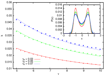
Figure 1: (color online) Plot of barrier crossing rate $k$ as a function of dissipation constant $\gamma$ for various values of the effective correlation time $\tau_{R}$. The solid lines are drawn from the theoretical expression, Eq.(60) and the symbols are the results of numerical simulation of Eq.(22). The values of the parameters used are $k_{B}T=D_{e}=0.05$, $\tau_{e}=0.04\text{ (red: solid)},0.06\text{ (green: dash)}\text{ and }0.08\text{ (blue: dot)}$ and $\kappa_{0}^{2}=3\text{ (red: solid)},5\text{ (green: dash)}\text{ and }7\text{ (blue: dot)}$. Inset: The normalized steady state PDF [ Eq.(59) ] using $\gamma=5.0$ and the same parameter set as in the main figure.

V Numerical implementation

To check the validity of our analytical result we numerically simulate the Langevin equation, Eq. (22) using Heun’s algorithm heun . In our simulation, we have always used a small integration step $\Delta t=0.001$ to ensure numerical stability. In addition to that all our numerical results have been averaged over 10, 000 trajectories to obtain a smooth numerical profile. As mentioned in Sec.II, although we mention the explicit values of the external noise parameters ($D_{e}$ and $\tau_{e}$) used in the simulation, we interpret our results in terms of the effective noise parameters $D_{R}$ and $\tau_{R}$.

In Fig.(1) we show the profile of escape rate, $k$ as a function of the dissipation constant, $\gamma$ for different values of the effective correlation time, $\tau_{R}$. Numerically, the escape rate has been defined as the inverse of the mean first passage time mfpt . The values of the different parameters used in the simulation are given in the figure caption. The profiles show that the numerical results are in good agreement with the analytical ones. As expected for a fixed $\tau_{R}$ value, the escape rate decreases with $\gamma$ but for a fixed value of $\gamma$, the escape rate increases with the increase of the effective correlation time, $\tau_{R}$. To understand this behavior we numerically calculate the steady state PDF mfpt for a fixed value of $\gamma$, which is a measure of the dynamics in the bistable potential. The analytical [ Eq.(59) ] and numerical profiles of steady state PDF [see the inset of Fig.(1)] show that the barrier height decreases as $\tau_{R}$ increases which effectively increases the escape rate, $k$. In Fig.(2) we show the variation of the escape rate with different values of the coupling term $\kappa_{0}$ which reflects an increasing trend of $k$ with $\kappa_{0}$. The steady state PDF profile accounts for this behavior with decrease in the barrier height [see the inset].

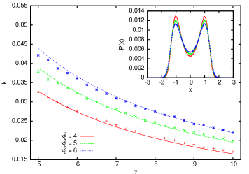
Figure 2: (color online) Plot of barrier crossing rate $k$ as a function of dissipation constant $\gamma$ for various values of coupling parameter $\kappa_{0}^{2}$. The solid lines are drawn from the theoretical expression, Eq.(60) and the symbols are the results of numerical simulation of Eq.(22). The values of the parameters used are $k_{B}T=D_{e}=0.05$ and $\tau_{e}=0.0625\text{ (red: solid)},0.06\text{ (green: dash)}\text{ and }0.0583\text{ (blue: dot)}$ so that the effective correlation time $\tau_{R}$ always remains 0.05. Inset: The normalized steady state PDF [ Eq.(59) ] using $\gamma=5.0$ and the same parameter set as in the main figure.

VI Conclusion

A system reservoir model, where the reservoir is modulated externally by a Gaussian colored noise has been proposed to study the transport of an overdamped Brownian particle in a periodic potential. Based on the Fokker-Planck-Smoluchowski description we calculate the mobility of the Brownian particle in the linear response regime and using Einstein’s relation the diffusion rate is calculated for any arbitrary periodic potential where the external driving noise is colored. For a cosine potential we obtain the diffusion rate in a closed analytical form and observe that the diffusion rate increases from white to colored noise. As an immediate application of our formalism, we study the bistable kinetics of the Brownian particle and demonstrate the dependence of the correlation time of the external colored noise, by which the bath is modulated, on the steady state probability density function and observe the barrier crossing dynamics to obtain the expression for escape rate. Our analytical result for the escape rate is then compared with the Langevin simulation result which shows that both are in very good agreement. To the end it should be noted that nonlinear system reservoir coupling may also be considered to obtain a Langevin equation for a Brownian particle effectively driven by a state dependent colored noise, from which one may observe various dynamical and kinematical aspects of the Brownian particle. We hope to address these issues in near the future.

- (1) A. Barone and G. Paterb, Physics and Applications of the Josephson Effects, (Wiley, NY, 1982).
- (2) J. W. M. Frenken and J. F. Vander Veen, Phys. Rev. Lett. 54, 134 (1985).
- (3) H. Sakaguchi, Prog. Theor. Phys. 79, 39 (1987).
- (4) H. Risken, The Fokker-Planck Equation (Springer-Verlag, Berlin, 1989); F. Jülicher, A. Ajdari and J. Prost, Rev. Mod. Phys. 69, 1269 (1997) and references therein.
- (5) P. Reimann, C. Van den Broeck, H. Linke, P. Hänggi, J. M. Rubi, and A. Pérez-Madrid, Phys. Rev. E 65, 031104 (2002); D. Dan and A. M. Jayannavar, Phys. Rev. E 66, 041106 (2002).
- (6) S. Leiber, Nature (London) 370, 412 (1994); J. Maddox, Nature (London) 365, 203 (1993); ibid 368, 287 (1994).
- (7) M. Borromeo and F. Marchesoni, Phys. Rev. E 73, 016142 (2006).
- (8) M. O. Magnasco, Phys. Rev. Lett. 71, 1477 (1993); P. Jung, J. G. Kissner and P. Hänggi, Phys. Rev. Lett. 76, 3436 (1996); R. Bartussek, P. Hänggi and J. G. Kissner, Europhys. Lett. 28, 459 (1994); S. Savel’ev, F. Marchesoni, and F. Nori, Phys. Rev. E 71, 011107 (2005).
- (9) J. Prost, J.-F. Chauwin, L. Peliti, and A. Ajdari, Phys. Rev. Lett. 72, 2652 (1994); J. Rousselet, L. Salome, A. Ajdari and J. Prost, Nature (London) 370, 446 (1994); J.-F. Chauwin, A. Ajdari and J. Prost, Europhys. Lett. 32, 373 (1995).
- (10) M. Borromeo, G. Costantini, and F. Marchesoni, Phys. Rev. E 65, 041110 (2002),
- (11) P. Reimann, R. Bartussek, R. Häussler and P. Hänggi, Phys. Lett. A 215, 26 (1996).
- (12) P. Reimann and P. Hänggi, Appl. Phys. A 75, 169 (2002); J. M. R. Parrondo and B. J. de Cisneros, Appl. Phys. A 75, 179 (2002); H. Wang and G Oster, Appl. Phys. A 75, 315 (2002); R. Lipowsky, Y. Chai, S. Klumpp, S. Liepelt, and Melanie J.I. Müller, Physica A 372, 34 (2006); D. Chowdhury, Physica A 372, 84 (2006); G. I. Menon, Physica A 372, 96 (2006).
- (13) J. Howard, Mechanics Of Motor Proteins and the Cytoskeletons, (Sinauer Associates, Sunderland, 2001).
- (14) P. J. Struman, Photovoltaic and Photoreflective Effects in Nanocentrosymmetric Materials, (Gordan and Breach, Philadelphia, 1992).
- (15) C. R. Doering, W. Horsthemke and J. Riordan, Phys. Rev. Lett. 72, 2984 (1994).
- (16) A. Ajdari, D. Mukamel, L. Peliti and J. Prost, J. Phys. I (France) 14, 1551 (1994); M. C. Mahato and A. M. Jayannavar, Phys. Lett. A 209, 21 (1995).
- (17) M. M. Millonas, Phys. Rev. Lett. 74, 10 (1995).
- (18) M. Büttiker, Z. Phys. B: Condensed Matter 68, 161 (1987).
- (19) A. V. Chechkin, O. Y. Sliusarenko, R. Metzler, and J. Klafter, Phys. rev. E 75, 041101 (2007) and references therein; D. del-Castillo-Negrete, V. Yu. Goncharb, and A. V. Chechkin, Physica A, doi:10.1016/j.physa.2008.08.034 (online edition)
- (20) M. Lax, Rev. Mod. Phys. 38, 541 (1966).
- (21) H. Risken, The Fokker-Planck Equation (Springer, Berlin, 1989).
- (22) R. Kubo, M. Toda, N. Hashitsume, and N. Saito, Statistical Physics II: Non-equilibrium Statistical Mechanics (Springer, Berlin, 1995).
- (23) K. Lindenberg and B. J. West, The Nonequilibrium Statistical Mechanics of Open and Closed Systems (VCH, New York, 1990).
- (24) J. Mencia Bravo, R. M. Velasco, and J. M. Sancho, J. Math. Phys. 30, 2023 (1989).
- (25) J. Ray Chaudhuri, S. K. Banik, B. C. Bag, and D. S. Ray, Phys. Rev. E. 63, 061111 (2001).
- (26) J. Ray Chaudhuri, D. Barik, and S. K. Banik, Phys. Rev. E 73, 051101 (2006).
- (27) J. Ray Chaudhuri, D. Barik, and S. K. Banik, Phys. Rev. E 74, 061119 (2006).
- (28) J. Ray Chaudhuri, D. Barik, and S. K. Banik, J. Phys. A 40, 14715 (2007).
- (29) J. Ray Chaudhuri, S. Chattopadhyay, and S. K. Banik, J. Chem. Phys. 127, 224508 (2007).
- (30) R. Hernandez and F. L. Somer, J. Phys. Chem. B, 103, 1070 (1999); A. N. Drozdov and S. C. Tucker, J. Phys. Chem. B 105, 6675 (2001); E. Hershkovits and R. Hernandez, J. Chem Phys. 122, 014509 (2005).
- (31) W. Horsthemke and R. Lefever, Noise-induced transitions: Theory and applications in physics, chemistry, and biology (Springer-Verlag, Berlin and New York, 1984).
- (32) D. A. Leigh, J. K. Y. Wong, F. Dehez and F. Zerbetto, Nature 424, 174 (2003).
- (33) K. Faid and R. F. Fox, Phys. rev. A 35, 2684 (1987).
- (34) M. Mañas, J. M. R. Parrondo and F. J. de La Rubia, J. Stat. Phys. 71, 1157 (1993).
- (35) I. M. Kulić, R. Thaokar, and H. Schiessel, Europhys. Lett., 72 (4), 527 (2005).
- (36) C. Mao, W. Sun, Z. Shen, and N. C. Seeman, Nature, 397, 144 (1999).
- (37) A. Ashkin, Phys. Rev. Lett. 24, 156, (1970)
- (38) K. Svoboda, S. M. Block, Annual Reviews of Biophysics and Biomolecular Structure 23, 247 (1994).
- (39) See for example, J. K. Bhattacharjee, Statistical Physics,: Equilibrium and Non-equilibrium Aspects (Allied Publishers, Kolkata, 2002)
- (40) M. San Miguel and J. M. Sancho, J. Stat. Phys. 22, 605 (1980).
- (41) R. Zwanzig, J. Stat. Phys. 9, 215 (1973); M. I. Dykman and M. A. Krivoglaz, Phys. Status Solidi B 48, 497 (1971).
- (42) L. D. Landau and E. M. Lifshitz, The Classical Theory of Fields (Pergamon, Oxford, 1975).
- (43) J. M. Moix and R. Hernandez, j. Chem. Phys. 122, 114111 (2005).
- (44) P. Resibois and M. dc Leener, Chemical Kinetic Theory of Fluids (Wiley-Interscience, NY, 1977).
- (45) P. Hänggi, P. Talkner, and M. Borkovec, Rev. Mod. Phys. 62, 251 (1990).
- (46) C. W. Gardiner, Handbook of Stochastic Methods (Springer, Berlin, 1985).
- (47) J. Garcia-Ojalvo and J. M. Sancho, Noise in Spatially Extended System (Springer, New York, 1999).
- (48) C. Mahanta and T. G. Venkatesh, Phys. Rev. E 58, 4141 (1998); D. Barik, B. C. Bag, and D. S. Ray, J. Chem. Phys. 119, 12973 (2003).