Contributions to Khovanov Homology

Abstract

Khovanov homology ist a new link invariant, discovered by M. Khovanov [Kh1], and used by J. Rasmussen [Ra] to give a combinatorial proof of the Milnor conjecture. In this thesis, we give examples of mutant links with different Khovanov homology. We prove that Khovanov’s chain complex retracts to a subcomplex, whose generators are related to spanning trees of the Tait graph, and we exploit this result to investigate the structure of Khovanov homology for alternating knots. Further, we extend Rasmussen’s invariant to links. Finally, we generalize Khovanov’s [Kh3] categorifications of the colored Jones polynomial, and study conditions under which our categorifications are functorial with respect to colored framed link cobordisms. In this context, we develop a theory of Carter–Saito movie moves for framed link cobordisms.

Introduction

In his seminal paper [Kh1], M. Khovanov introduced a new invariant for oriented knots and links, which can be viewed as a “categorification” of the Jones polynomial [Jo]. To a diagram $D$ of an oriented link $L\subset\mathbb{R}^{3}$, Khovanov assigned a bigraded chain complex $\mathcal{C}^{i,j}(D)$ whose differential is graded of bidegree $(1,0)$, and whose homotopy type depends only on the isotopy class of the oriented link $L$. The graded Euler characteristic

$$\chi_{q}(\mathcal{C}(D)):=\sum_{i,j}(-1)^{i}q^{j}\dim_{\mathbb{Q}}(\mathcal{C}^{i,j}(D)\otimes\mathbb{Q})\,\in\mathbb{Z}[q,q^{-1}]$$

is a suitably normalized version of the Jones polynomial of $L$:

$$V(L)_{\sqrt{t}=-q}=\frac{\chi_{q}(\mathcal{C}(D))}{q+q^{-1}}$$

The bigraded homology group $\mathcal{H}^{i,j}(D)$ of the chain complex $\mathcal{C}^{i,j}(D)$ provides an invariant of oriented links, now known as Khovanov homology. Because Khovanov’s construction is manifestly combinatorial, Khovanov homology is algorithmically computable.

One of the remarkable properties of Khovanov homology is that it fits into a topological quantum field theory of $2$–knots in $4$–space. Indeed, any smooth link cobordism $S\subset\mathbb{R}^{3}\times[0,1]$ between two oriented links $L_{0}\times\{0\}$ and $L_{1}\times\{1\}$ induces a chain transformation $\mathcal{C}(S):\mathcal{C}(D_{0})\rightarrow\mathcal{C}(D_{1})$, which is a relative isotopy invariant of the cobordism $S$ when considered up to sign and homotopy. Moreover, $\mathcal{C}(S)$ is graded of bidegree $(0,\chi(S))$, where $\chi(S)$ denotes the Euler characteristic of the surface $S$.

In [L2], E. S. Lee modified Khovanov’s construction by adding additional terms to the differential. On the basis of Lee’s results, J. Rasmussen [Ra] defined a new knot invariant $s(K)\in\mathbb{Z}$ and used it to give a purely combinatorial proof of Milnor’s conjecture on the slice genus of torus knots. Previously, this conjecture had been accessible only via Donaldson invariants, Seiberg–Witten theory and knot Floer homology, and was considered as a main application of these theories. In many ways, Khovanov homology appears to be an algebro–combinatorial replacement for gauge theory and Heegaard Floer homology. An explicit relation between reduced Khovanov homology with coefficients in $\mathbb{Z}/2\mathbb{Z}$ and Heegaard Floer homology of branched double–covers of the $3$–sphere, in the form of a spectral sequence, was discovered by P. Ozsváth and Z. Szabó [OS2].

In the past few years, several new link homology theories have emerged. Among these are the Khovanov–Rozansky theories for the $\mathfrak{sl}(n)$ polynomials and the HOMFLY–PT polynomial [KR1, KR2], and two categorifications of the colored Jones polynomial, proposed by Khovanov [Kh3]. Moreover, D. Bar–Natan [B2] discovered a “formal Khovanov bracket”, which generalizes both Khovanov homology and Lee homology, and which extends naturally to tangles.

This thesis is devoted to the study of structural properties of Khovanov homology, as well as to the generalization of Rasmussen’s invariant and its applications, and contains contributions towards a $4$–dimensional lift of Khovanov’s theory for the colored Jones polynomial.

In Chapter 1 we review the definition of the formal Khovanov bracket and discuss its relation with Khovanov homology and Lee homology.

Chapter 2 deals with Rasmussen’s invariant. We give a new proof of a theorem of E. S. Lee [L2], which states that the Lee homology of an $n$–component link has dimension $2^{n}$. Then we extend Rasmussen’s knot invariant to links, and give examples where this invariant is a stronger obstruction to sliceness than the multivariable Levine–Tristram signature.

In Chapter 3, we study the behavior of Khovanov homology under Conway mutation. Conway mutation is a procedure for modifying links, which was invented by J. Conway [Co]. We present infinitely many examples of mutant links with different Khovanov homology. The existence of such examples is remarkable since many classical invariants, such as the HOMFLY–PT polynomial, the knot signature and the hyperbolic volume of the knot complement, are unable to detect Conway mutation. In particular, our examples show that Khovanov homology is strictly stronger than the Jones polynomial.

In [B1], Bar–Natan computed the ranks of the Khovanov homology groups for all prime knots with up to 11 crossings. One of his surprising experimental results is that the ranks of the Khovanov homology groups tend to be much smaller than the ranks of the chain groups. In Chapter 4 we give an explanation for this phenomenon: we prove that the complex $\mathcal{C}^{i,j}(D)$ retracts to a subcomplex, whose generators are in $2:1$ correspondence with the spanning trees of the Tait graph of $D$. Using this result, we give a new proof of a theorem of Lee [L1], which states that the non–trivial homology groups $\mathcal{H}^{i,j}(K)$ of an alternating knot $K$ are concentrated on two straight lines in the $ij$–plane. Our spanning tree model has applications to Legendrian knots (cf. [Wu]), and it is of theoretical interest because spanning trees also appear in the context of knot Floer homology [OS1].

Chapter 5 is purely topological. We investigate link cobordisms equipped with a framing, i.e. with a relative homotopy class of non–singular normal vector fields. The most important part of Chapter 5 is the last section, where we give a list of movie moves for movie presentations of framed link cobordisms. Framed movie moves are needed if one wishes to establish functoriality of colored Khovanov invariants [Kh3] with respect to framed link cobordisms.

In Chapter 6, we focus on Khovanov’s [Kh3] categorification of the non–reduced colored Jones polynomial. By reformulating Khovanov’s construction in Bar–Natan’s setting, we obtain a “colored Khovanov bracket”. We prove that the colored Khovanov bracket is well–defined over integer coefficients. Moreover, we introduce a family of modified colored Khovanov brackets, and study conditions under which our modified theories are functorial with respect to colored framed link cobordisms. Lifting the colored Jones polynomial to a functor can be seen as a first step into the direction of categorification of the $\mathfrak{sl}(2)$ quantum invariant for $3$–manifolds, and might ultimately lead to an intrinsically $3$– or $4$–dimensional understanding of Khovanov homology.

The material of Chapter 1 is taken from [B2], [B3], [Kh1], [Kh4], [L2] and [We2]. Chapters 2, 5 and 6 contain the results of my joint paper with A. Beliakova [BW], and Chapters 3 and 4 are taken from [We1] and [We2].

Acknowledgements

First and foremost, I would like to thank my supervisors Anna Beliakova and Norbert A’Campo for their constant support and encouragement, and for their readiness to share their advice and expertise with me. I would also like to thank Sebastian Baader, Mikhail Khovanov and Alexander Shumakovitch for their interest in this work and for many valuable discussions. Dror Bar–Natan’s symbol font dbnsymb was used throughout this thesis. The material covered in Chapters 2, 5 and 6 is taken from my joint work with Anna Beliakova. During the work on this thesis, I was partially supported by the Swiss National Science Foundation.

Chapter 1 Khovanov homology

In this chapter, we first recall basic concepts of knot theory. Then we give the definitions of the Jones polynomial and the formal Khovanov bracket, and discuss how Khovanov homology and Lee homology can be recovered from the Khovanov bracket by applying a TQFT.

1.1 Links and link cobordisms

A link in $\mathbb{R}^{3}$ is a finite collection of disjoint circles which are smoothly embedded into $\mathbb{R}^{3}$. These circles are called the components of the link. If an orientation of the components is specified, we say that the link is oriented. For an oriented link $L$, we denote by $-L$ the same link but with reversed orientations. A link consisting of only one component is called a knot.

Figure 1.1: An oriented link diagram.

To present links, one uses pictures such as the one in Figure 1.1, called link diagrams. Given an oriented link diagram $D$, we denote by $c_{+}(D)$ and $c_{-}(D)$ the numbers its positive () and negative () crossings, and by $w(D):=c_{+}(D)-c_{-}(D)$ the writhe of $D$. (E.g. in the above figure we have $w(D)=-c_{-}(D)=-3$ and $c_{+}(D)=0$).

It is known that two link diagrams represent isotopic links if and only if they are related by a finite sequence of the following local modifications, called Reidemeister moves.

Figure 1.2: The three Reidemeister moves R1, R2 and R3.

To classify links up to isotopy, one usually uses link invariants, i.e. functions whose domain is the set of links in $\mathbb{R}^{3}$ and whose value depends only on the isotopy class of a link. One way of constructing a link invariant is by defining it on the level of link diagrams and then showing that it is invariant under Reidemeister moves.

A cobordism between two oriented links $L_{0}$ and $L_{1}$ is a compact oriented surface smoothly embedded in $\mathbb{R}^{3}\times[0,1]$ whose boundary lies entirely in $\mathbb{R}^{3}\times\{0,1\}$ and whose “bottom” boundary is $-L_{0}\times\{0\}$ and whose “top” boundary is $L_{1}\times\{1\}$. For technical reasons, we assume that the surface is in general position with respect to the projection onto the last coordinate of $\mathbb{R}^{3}\times[0,1]$, and parallel to $[0,1]$ near the boundary. It convenient to view the last coordinate of $\mathbb{R}^{3}\times[0,1]$ as time coordinate.

Assume $S\subset\mathbb{R}^{3}\times[0,1]$ is a link cobordism. By cutting $S$ along hyperplanes $\mathbb{R}^{3}\times\{t_{i}\}$, $0=t_{0}<t_{1}<\ldots<t_{n}=1$, we can split $S$ into elementary pieces, such that each piece $S\cap\mathbb{R}^{3}\times[t_{i-1},t_{i}]$ contains at most one critical point with respect to the time coordinate, and such that all $t_{i}$ are regular values. Projecting the oriented links $L_{t_{i}}:=S\cap(\mathbb{R}^{3}\times\{t_{i}\})$ down to the plane, we obtain a sequence of oriented link diagrams $D_{t_{i}}$. Altering the $t_{i}$, we can assume that any two consecutive diagrams differ by one of the following transformations: a planar isotopy, a Reidemeister move, or one of the Morse moves shown in Figure 1.3. In this case, the sequence $\{D_{t_{i}}\}$ is called a movie presentation for $S$, and the individual diagrams $D_{t_{i}}$ are called the stills of the movie presentation.

Figure 1.3: Morse moves corresponding to cap, cup and saddle cobordism.

Theorem 1 ([CS])

1. Every link cobordism has a movie presentation. 2. Two movies represent isotopic link cobordisms if and only if they can be transformed into each other by a finite sequence of Carter–Saito movie moves (and by time–reordering different parts of a movie which “happen” at different places).

The Carter–Saito movie moves are shown in Figures 1.4, 1.5 and 1.6. The moves of Type I and II consist in replacing the circular movies of Figures 1.4 and 1.5 by identity movies, i.e. by movies where all stills look the same.

Figure 1.4: Type I moves.

Figure 1.5: Type II moves.

Figure 1.6: Type III moves.

As it will be needed in Chapter 5, we briefly recall the definition of the linking number. Let $L=K_{1}\cup K_{2}$ be an oriented $2$–component link with corresponding diagram $D=D_{1}\cup D_{2}$. Let $c_{+}^{\prime}(D)$ and $c_{-}^{\prime}(D)$ denote the numbers of positive and negative crossings at which $D_{1}$ and $D_{2}$ cross. Note that $c_{+}^{\prime}(D)$ and $c_{-}^{\prime}(D)$ have the same parity, because $D_{1}$ and $D_{2}$ necessarily cross in an even number of crossings.

The linking number of $K_{1}$ and $K_{2}$ is defined by

$$\operatorname{lk}(K_{1},K_{2}):=(c_{+}^{\prime}(D)-c_{-}^{\prime}(D))/2\,\in\mathbb{Z}\;.$$

It is easy to see that $\operatorname{lk}(K_{1},K_{2})$ is invariant under Reidemeister moves and hence determines an invariant of the link $L$. Geometrically, the linking number can be interpreted as the algebraic intersection number of two generic compact oriented surfaces $S_{1},S_{2}\subset\mathbb{R}^{3}\times(\infty,0]$ satisfying $\partial S_{i}=K_{i}\times\{0\}\subset\mathbb{R}^{3}\times\{0\}$.

1.2 The Kauffman bracket and the Jones polynomial

The Jones polynomial is an invariant for oriented links which was introduced by V. Jones [Jo] in the year 1984. In [Ka2], L. Kauffman described an elementary approach to the Jones polynomial using a state sum. In this section, we recall Kauffman’s definition of the Jones polynomial. We use the normalization conventions of [Kh1].

Let $D$ be an unoriented link diagram. A Kauffman state of $D$ is a diagram obtained by replacing each crossing of $D$ with or (so that the result is a disjoint union of circles embedded in the plane). We denote by ${\mathcal{K}}(D)$ the set of all Kauffman states of $D$, and by $n(D^{\prime})$ the number of circles in $D^{\prime}\in{\mathcal{K}}(D)$. If $D$ has $c$ crossings, the number of Kauffman states is $2^{c}$. Given a crossing of $D$ (looking like this: ), we call its $0$–smoothing and its $1$–smoothing. We denote by $r(D,D^{\prime})$ the number of $1$–smoothings in $D^{\prime}$, where here $D^{\prime}$ can be a Kauffman state of $D$ or more generally any link diagram obtained from $D$ by smoothing some of the crossings while leaving the others unchanged.

The Kauffman bracket of $D$ is the Laurent polynomial $\langle D\rangle\in\mathbb{Z}[q,q^{-1}]$ defined by

$$\langle D\rangle:=\sum_{D^{\prime}\in{\mathcal{K}}(D)}(-q)^{r(D,D^{\prime})}(q+q^{-1})^{n(D^{\prime})}.$$ (1.1)

For example, the Kauffman bracket of a crossingless diagram $D=\bigcirc^{n}$ consisting of $n$ disjoint circles is just $\langle\bigcirc^{n}\rangle=(q+q^{-1})^{n}$. Setting $\langle D|D^{\prime}\rangle:=(-q)^{r(D,D^{\prime})}$, we can rewrite the above formula as

$$\langle D\rangle:=\sum_{D^{\prime}\in{\mathcal{K}}(D)}\langle D|D^{\prime}\rangle\langle D^{\prime}\rangle\;.$$ (1.2)

It is easy to see that the Kauffman bracket satisfies the following rules:

$$\langle\emptyset\rangle = 1,$$ (1.3)

$$\langle D\sqcup\bigcirc\rangle = (q+q^{-1})\langle D\rangle,$$ (1.4)

$$\langle\slashoverback\rangle = \langle\smoothing\rangle-q\langle\hsmoothing\rangle.$$ (1.5)

Rule (1.3) says that the empty link evaluates to $1$. Rule (1.4) says that $\langle D\rangle$ is multiplied by $(q+q^{-1})$ when a disjoint circular component is added to $D$. In the third rule, the three pictures , and stand for three link diagrams which are identical except in a small disk, where they look like , and , respectively. The above rules determine the Kauffman bracket completely (see Chapter 4).

Using (1.4) and (1.5) one can prove the following lemma which shows that the Kauffman bracket is invariant under Reidemeister moves when considered up to multiplication with a unit of the ring $\mathbb{Z}[q,q^{-1}]$.

Lemma 1

The Kauffman bracket satisfies

1. $\langle{\begin{array}[]{c}\raisebox{-2.5pt}{\includegraphics[height=12.0pt]{figs/leftRI.eps}}\end{array}}\rangle=q^{-1}\langle{\begin{array}[]{c}\raisebox{-2.5pt}{\includegraphics[height=12.0pt]{figs/noRI.eps}}\end{array}}\rangle$ and $\langle{\begin{array}[]{c}\raisebox{-2.5pt}{\includegraphics[height=12.0pt]{figs/rightRI.eps}}\end{array}}\rangle=-q^{2}\langle{\begin{array}[]{c}\raisebox{-2.5pt}{\includegraphics[height=12.0pt]{figs/noRI.eps}}\end{array}}\rangle$.

2. $\langle{\begin{array}[]{c}\raisebox{-2.5pt}{\includegraphics[height=12.0pt]{figs/RII.eps}}\end{array}}\rangle=-q\langle{\begin{array}[]{c}\raisebox{-2.5pt}{\includegraphics[height=12.0pt]{figs/noRII.eps}}\end{array}}\rangle$.

3. $\langle{\begin{array}[]{c}\raisebox{-2.5pt}{\includegraphics[height=14.0pt]{figs/RIIIa.eps}}\end{array}}\rangle=\langle{\begin{array}[]{c}\raisebox{-2.5pt}{\includegraphics[height=14.0pt]{figs/RIIIb.eps}}\end{array}}\rangle$.

If $D$ is the diagram of an oriented link $L$, we can define

$$J(D):=(-1)^{c_{-}(D)}q^{c_{+}(D)-2c_{-}(D)}\langle D\rangle.$$ (1.6)

Lemma 1 implies that $J(D)$ is invariant under Reidemeister moves and hence an invariant of the link $L$. We denote this invariant by $J(L)$ and call it the Jones polynomial of $L$. The normalization of $J(L)$ is chosen so that

$$J(\emptyset)=1\qquad\text{and}\qquad J(\bigcirc)=q+q^{-1}.$$ (1.7)

A triple $(L_{+},L_{-},L_{0})$ of oriented links is called a skein triple if the oriented links $L_{+}$, $L_{-}$ and $L_{0}$ possess diagrams which are mutually identical except in a small disc, where they look like , and , respectively. Using rule (1.5), it is easy to see that the Jones polynomial satisfies

$$q^{-2}J(L_{+})-q^{2}J(L_{-})=(q^{-1}-q)J(L_{0})$$ (1.8)

for any skein triple $(L_{+},L_{-},L_{0})$. It is known that the Jones polynomial is determined uniquely by relations (1.7) and (1.8) and the fact that it is a link invariant.

Relation (1.8) implies that the value of the Jones polynomial depends only on the skein equivalence class of a link, where skein equivalence is defined as follows:

Definition 1 ([Kaw])

The skein equivalence is the minimal equivalence relation “$\sim$” on the set of oriented links satisfying $L\sim L^{\prime}$ whenever $L$ and $L^{\prime}$ are isotopic and such that

1. $L_{0}\sim L^{\prime}_{0}$ and $L_{-}\sim L^{\prime}_{-}$ imply $L_{+}\sim L^{\prime}_{+}$,

2. $L_{0}\sim L^{\prime}_{0}$ and $L_{+}\sim L^{\prime}_{+}$ imply $L_{-}\sim L^{\prime}_{-}$,

for any two skein triples $(L_{+},L_{-},L_{0})$ and $(L^{\prime}_{+},L^{\prime}_{-},L^{\prime}_{0})$.

The Laurent polynomials $\langle D\rangle$ and $J(L)$ defined as above are related to the original Kauffman bracket $\langle D\rangle^{\operatorname{ori}}$ and Jones polynomial $V(L)$ by

$$\left[A^{-c}\langle D\rangle^{\operatorname{ori}}\right]_{A^{-2}=-q}=\langle D\rangle\qquad\text{and}\qquad V(L)_{\sqrt{t}=-q}=\frac{J(L)}{q+q^{-1}},$$

where $c$ denotes the number of crossings of $D$.

1.3 Bar–Natan’s formal Khovanov bracket

Khovanov homology was discovered by M. Khovanov [Kh1] in the year 1999. In [B2], D. Bar–Natan proposed a generalization of Khovanov’s invariant, which he called the formal Khovanov bracket.

In Subsections 1.3.1, 1.3.2, 1.3.3 and 1.3.4, we explain the target category for the formal Khovanov bracket. Notice that the category ${\mathcal{C}ob}_{\bullet/l}^{3}$ used in this thesis is not the original category of [B2]. It is similar though to a category introduced in [B2, Section 11], but more general and more directly related to Khovanov’s universal rank $2$ Frobenius system [Kh4]. In Subsections 1.3.5 and 1.3.6, we review the definition of the formal Khovanov bracket and discuss how the formal Khovanov bracket extends to tangles.

1.3.1 Complexes in additive categories.

Let $\mathcal{C}$ be an additive category. A bounded (co)chain complex in $\mathcal{C}$ is a sequence of objects and morphisms of $\mathcal{C}$

$$K:\quad\ldots\;\longrightarrow\hskip 6.50403ptK^{i}\hskip 6.50403pt\stackrel{{\scriptstyle d_{K}^{i}}}{{\longrightarrow}}\hskip 6.50403ptK^{i+1}\hskip 6.50403pt\stackrel{{\scriptstyle d_{K}^{i+1}}}{{\longrightarrow}}\hskip 6.50403ptK^{i+2}\hskip 6.50403pt\longrightarrow\;\ldots$$

with the property that $d_{K}^{i+1}\circ d_{K}^{i}=0$ for all $i\in\mathbb{Z}$ and $K^{i}=0$ for all but finitely many $i\in\mathbb{Z}$. A chain transformation $f:K\rightarrow L$ between two complexes $K$ and $L$ in $\mathcal{C}$ is a sequence of morphisms $f^{i}:K^{i}\rightarrow L^{i}$ such that $d_{K}^{i}\circ f^{i}=f^{i+1}\circ d_{L}^{i+1}$ for all $i\in\mathbb{Z}$. Two chain transformations $f,g:K\rightarrow L$ are called homotopic if there exists a chain homotopy between them, i.e. a sequence of morphisms $h^{i}:K^{i}\rightarrow L^{i-1}$ such that $d_{L}^{i-1}\circ h^{i}+h^{i+1}\circ d_{K}^{i}=f^{i}-g^{i}$. Let $\operatorname{Kom}(\mathcal{C})$ denote the category whose objects are bounded complexes in $\mathcal{C}$ and whose morphisms are chain transformations, and let $\operatorname{Kom}_{/h}(\mathcal{C})$ denote the quotient category $\operatorname{Kom}(\mathcal{C})/\mathcal{N}$ where $\mathcal{N}$ is the ideal of chain transformations homotopic to $0$.

Two complexes in $\mathcal{C}$ are said to be isomorphic (homotopic) if they are isomorphic as objects of $\operatorname{Kom}(\mathcal{C})$ ($\operatorname{Kom}_{/h}(\mathcal{C})$). A complex which is homotopic to the trivial complex is called contractible. Equivalently, a complex $K$ is contractible if its identity morphism $\operatorname{Id}_{K}:K\rightarrow K$ is homotopic to $0$.

Given a complex $K=(K^{i},d_{K}^{i})$, we refer to the index $i$ as the homological degree. For every $n\in\mathbb{Z}$ we denote by $[n]$ the endofunctor of $\operatorname{Kom}(\mathcal{C})$ which raises the homological degree by $n$, i.e. $K[n]^{i+n}=K^{i}$ and $d_{K[n]}^{i+n}=d_{K}^{i}$. (Note that our convention is opposite to the convention used in [Kh1]).

Given a chain transformation $f:K\rightarrow L$, the mapping cone of $f$ is the complex $\Gamma(f):=K\oplus L[1]$ with the differential

$$d_{\Gamma(f)}:=\begin{pmatrix}d_{K}&0\\ f&-d_{L[1]}\end{pmatrix}$$

i.e. $d_{\Gamma(f)}(x,y)=(d_{K}x,fx-d_{L[1]}y)$ for all $(x,y)\in K\oplus L[1]$. It is easy to see that the mapping cone of an isomorphism is always contractible. Indeed, if $f$ is an isomorphism, we can define a homotopy between $\operatorname{Id}_{\Gamma(f)}$ and $0$ by

$$h=\begin{pmatrix}0&f^{-1}\\ 0&0\end{pmatrix}\;.$$

Let $K$ and $L$ be two complexes in $\mathcal{C}$. We say that $K$ destabilizes to $L$, or $L$ stabilizes to $K$, if $K$ is isomorphic to $L\oplus C$ for a complex $C$ which is isomorphic to the mapping cone of an isomorphism. Moreover, we say that two complexes $K$ and $L$ are stably isomorphic if they become isomorphic after stabilizing. The following lemma is taken from [We2, Lemma 2.1] (but see also [B2, Lemma 4.5]).

Lemma 2

Let $K$, $L$ be complexes such that $K=K_{1}\oplus K_{2}$ and $L=L_{1}\oplus L_{2}$ for contractible complexes $K_{2}$ and $L_{2}$. Then the mapping cone $\Gamma(f)$ of a chain transformation

$$\begin{CD}K=K_{1}\oplus K_{2}@>{\quad\;\mbox{f = }\begin{pmatrix}f_{11}&f_{12}\\ f_{21}&f_{22}\end{pmatrix}\quad\;}>{}>L_{1}\oplus L_{2}=L\end{CD}\vspace{0.05in}$$

is isomorphic to the complex $\Gamma(f_{11})\oplus K_{2}\oplus L_{2}[1]$. In particular, if $K_{2}$ and $L_{2}$ destabilize to the trivial complex, then $\Gamma(f)$ destabilizes to $\Gamma(f_{11})$.

Proof. On the level of objects (i.e. if one ignores the differentials), the complexes $\Gamma(f)$ and $\Gamma(f_{11})\oplus K_{2}\oplus L_{2}[1]$ are both isomorphic to $K\oplus L[1]$. Thus, to prove the lemma, it suffices to construct an automorphism $F:K\oplus L[1]\rightarrow K\oplus L[1]$ which intertwines the differentials. We define $F$ by

$$F=\begin{pmatrix}\operatorname{Id}_{K}&0\\ -N&\operatorname{Id}_{L}\end{pmatrix}$$

where $N:K_{1}\oplus K_{2}\rightarrow L_{1}[1]\oplus L_{2}[1]$ is given by

$$N=\begin{pmatrix}0&f_{12}h_{K}\\ h_{L}f_{21}&h_{L}f_{22}\end{pmatrix}$$

with $h_{K}$ and $h_{L}$ denoting the contracting homotopies of the complexes $K_{2}$ and $L_{2}$, respectively. A direct computation shows that $F\circ d_{\Gamma(f)}=(d_{\Gamma(f_{11})}+d_{K_{2}}+d_{L_{2}[1]})\circ F$, so $F$ is indeed an isomorphism between the complexes $\Gamma(f)$ and $\Gamma(f_{11})\oplus K_{2}\oplus L_{2}[1]$. $\Box$

If $K=(K^{i},d_{K}^{i})$ is a complex in a category of modules over a ring, one can define the $i$–th homology module of $K$ by $H^{i}(K):=(\operatorname{ker}d_{K}^{i})/(\operatorname{im}d_{K}^{i-1})$. It is easy to see that homotopic complexes have isomorphic homology modules.

1.3.2 Dotted cobordisms.

Let $D_{0}$, $D_{1}$ be two closed $1$–manifolds embedded in the plane $\mathbb{R}^{2}$. A cobordism from $D_{0}$ to $D_{1}$ is a compact orientable surface $S\subset\mathbb{R}^{2}\times[0,1]$ whose boundary lies entirely in $\mathbb{R}^{2}\times\{0,1\}$ and whose “bottom” boundary is $D_{0}\times\{0\}$ and whose “top” boundary is $D_{1}\times\{1\}$. A dotted cobordism is a cobordism which is decorated by finitely many distinct dots, lying in its interior. (These dots must not be confused with the signed points which will be introduced in Chapter 5). Dotted cobordisms can be composed by placing them atop of each other. We denote by ${\mathcal{C}ob}_{\bullet}^{3}$ the category whose objects are closed embedded $1$–manifolds and whose morphisms are dotted cobordisms, considered up to boundary–preserving isotopy.

We also define a quotient ${\mathcal{C}ob}_{\bullet/l}^{3}$ of ${\mathcal{C}ob}_{\bullet}^{3}$, as follows. ${\mathcal{C}ob}_{\bullet/l}^{3}$ has the same objects as ${\mathcal{C}ob}_{\bullet}^{3}$ but its morphisms are formal $\mathbb{Z}$–linear combinations of morphisms of ${\mathcal{C}ob}_{\bullet}^{3}$, considered modulo the following local relations:

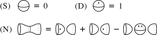
Figure 1.7: (S), (D) and (N) relation.

Relation (S) means that any cobordism, which has a sphere without dots among its connectivity components, is set to zero. Relation (D) means that a sphere decorated by a single dot can be removed from a cobordism without changing the class of the coborsism in ${\mathcal{C}ob}_{\bullet/l}^{3}$. Finally, (N) is the neck–cutting relation. It can be used to reduce the genus of a cobordism, at the expense of introducing some extra dots. Note that (S), (D) and (N) imply the following relations:

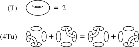
Figure 1.8: (T) and (4Tu) relation.

If we impose the additional relation that a sphere decorated by exactly two dots is zero ( $\raisebox{-5.69046pt}{\psfig{height=17.07182pt}}=0$ ), then the (S) relation becomes a consequence of the relations (D) and (N). Moreover, forming the connected sum with a torus becomes equivalent to inserting a dot at the connected sum point and then multiplying by $2\in\mathbb{Z}$. Hence we essentially get back the theory of [B2, Section 11], [B3].

Notations. We will use the following notations for the generating morphisms of ${\mathcal{C}ob}_{\bullet/l}^{3}$. The symbol stands for a saddle cobordism from to . More specifically, stands for a saddle which splits a single component into two, and stands for a saddle which merges two components into one. $\fourwheel:\emptyset\rightarrow\bigcirc$ and $\fourinwheel:\bigcirc\rightarrow\emptyset$ denote the cup and the cap cobordism, and $\dotcircle:\bigcirc\rightarrow\bigcirc$ denotes the “multiplication” of $\bigcirc$ by a dot, i.e. the identity cobordism $\bigcirc\times[0,1]$ decorated by a single dot.

1.3.3 Jones grading.

In this subsection, we enhance the category ${\mathcal{C}ob}_{\bullet/l}^{3}$ by introducing a grading. We essentially follow [B2, Section 6].

Given a dotted cobordism $S$, we define its Jones degree by

$$\deg(S):=\chi(S)-2\delta(S)$$

where $\chi(S)$ denotes the Euler characteristic of $S$ and $\delta(S)$ denotes the number of dots on $S$. Since the (S), (D) and (N) relations are degree–homogeneous, the Jones degree descends to ${\mathcal{C}ob}_{\bullet/l}^{3}$, turning morphism sets of ${\mathcal{C}ob}_{\bullet/l}^{3}$ into graded $\mathbb{Z}$–modules.

We construct a graded category $({\mathcal{C}ob}_{\bullet/l}^{3})^{\prime}$. The objects of $({\mathcal{C}ob}_{\bullet/l}^{3})^{\prime}$ are pairs $(D,n)$, one for each object $D\in\operatorname{Ob}({\mathcal{C}ob}_{\bullet/l}^{3})$ and each integer $n\in\mathbb{Z}$. As ungraded $\mathbb{Z}$–modules, the morphism sets of $({\mathcal{C}ob}_{\bullet/l}^{3})^{\prime}$ are the same as in ${\mathcal{C}ob}_{\bullet/l}^{3}$, i.e.

$$\operatorname{Mor}((D_{0},n_{0}),(D_{1},n_{1})):=\operatorname{Mor}(D_{0},D_{1})\;.$$

But the Jones degree of $S\in\operatorname{Mor}((D_{0},n_{0}),(D_{1},n_{1}))$ is defined by

$$\deg(S):=\chi(S)-2\delta(S)+n_{1}-n_{0}\;.$$

Note that $\deg(S)$ is additive under composition of morphisms.

For $m\in\mathbb{Z}$, we denote by $\{m\}$ the endofunctor of $({\mathcal{C}ob}_{\bullet/l}^{3})^{\prime}$ which “raises the grading” by $m$, i.e. $(D,n)\{m\}:=(D,n+m)$. To simplify notations, we will write $D$ instead of $(D,0)$ (and consequently $D\{n\}$ instead of $(D,n)$).

In what follows, we suppress the prime from $({\mathcal{C}ob}_{\bullet/l}^{3})^{\prime}$ and just call it ${\mathcal{C}ob}_{\bullet/l}^{3}$. We denote by $\text{{g}}{\mathcal{C}ob}_{\bullet/l}^{3}$ the subcategory of ${\mathcal{C}ob}_{\bullet/l}^{3}$ which has the same objects as ${\mathcal{C}ob}_{\bullet/l}^{3}$, but whose morphisms are required to be graded of Jones degree $0$.

1.3.4 Additive closure and delooping.

For every pre–additive category $\mathcal{C}$, there is an associated additive category $\operatorname{Mat}(\mathcal{C})$, called its additive closure. The objects of $\operatorname{Mat}(\mathcal{C})$ are finite sequences $(\mathcal{O}_{i})_{i=1}^{n}$ of objects $\mathcal{O}_{i}\in\operatorname{Ob}(\mathcal{C})$, which we write as formal direct sums $\bigoplus_{i=1}^{n}\mathcal{O}_{i}$. The morphisms $F:\bigoplus_{j}\mathcal{O}_{j}\rightarrow\bigoplus_{i}\mathcal{O}^{\prime}_{i}$ are matrices $[F_{i,j}]$ of morphisms $F_{i,j}:\mathcal{O}_{j}\rightarrow\mathcal{O}^{\prime}_{i}$. Composition of morphisms is modeled on ordinary matrix multiplication:

$$[F\circ G]_{i,k}:=\sum_{j}F_{i,j}\circ G_{j,k}$$

The following lemma is Bar–Natan’s Lemma 4.1 [B3], with the only difference that we use a slightly more general definition for the category ${\mathcal{C}ob}_{\bullet/l}^{3}$.

Lemma 3

(Delooping) Let $D^{\prime}$ be an object in $\text{{g}}{\mathcal{C}ob}_{\bullet/l}^{3}$ containing a circle $\bigcirc$, and let $D$ be the object obtained by removing this circle from $D^{\prime}$. Then $D^{\prime}$ is isomorphic in $\operatorname{Mat}(\text{{g}}{\mathcal{C}ob}_{\bullet/l}^{3})$ to $D\{+1\}\oplus D\{-1\}$.

Proof. It suffices to show that the circle $\bigcirc$ is isomorphic to $\emptyset\{+1\}\oplus\emptyset\{-1\}$. The isomorphisms are given by

Using relations (S), (D) and (N), it is easy to see that the above morphisms are mutually inverse isomorphism. $\Box$

Let $\operatorname{Kob}:=\operatorname{Kom}(\operatorname{Mat}({\mathcal{C}ob}_{\bullet/l}^{3}))$ denote the category of bounded complexes in $\operatorname{Mat}({\mathcal{C}ob}_{\bullet/l}^{3})$, and $\operatorname{Kob}_{/h}:=\operatorname{Kom}_{/h}(\operatorname{Mat}({\mathcal{C}ob}_{\bullet/l}^{3}))$ its homotopy category. Likewise, let $\operatorname{gKob}:=\operatorname{Kom}(\operatorname{Mat}(\text{{g}}{\mathcal{C}ob}_{\bullet/l}^{3}))$ and $\operatorname{gKob}_{/h}:=\operatorname{Kom}_{/h}(\operatorname{Mat}(\text{{g}}{\mathcal{C}ob}_{\bullet/l}^{3}))$.

1.3.5 Definition of the Khovanov bracket.

Let $D$ be an unoriented link diagram with $c$ crossings. Recall that the Kauffman states of $D$ are the diagrams obtained by replacing every crossing of $D$ by its $0$–smoothing or its $1$–smoothing. After numbering the crossings of $D$, we can parametrize the Kauffman states of $D$ by $c$–letter strings of $0$’s and $1$’s, specifying the smoothing chosen at each crossing. Let $D_{s}$ denote the Kauffman state corresponding to the $c$–letter string $s\in\{0,1\}^{c}$, and let $r(s):=r(D,D_{s})$ and $n(s):=n(D_{s})$ denote respectively the number of $1$’s in $s$ and the number of circles in $D_{s}$. We can arrange the Kauffman states of $D$ at the vertices of a $c$–dimensional cube. In Figure 1.9, the cube is displayed in such a way that two vertices which have the same number of $1$’s (i.e. the same $r(s)$) lie vertically above each other.

Figure 1.9: The cube of resolutions for the trefoil.

Two vertices $s$ and $t$ are connected by an edge (directed from $s$ to $t$) if they differ by a single letter which is a $0$ in $s$ and a $1$ in $t$. For such $s$ and $t$ the corresponding Kauffman states $D_{s}$ and $D_{t}$ differ at a single crossing which is a $0$–smoothing in $D_{s}$ and a $1$–smoothing in $D_{t}$. To the edge connecting $s$ and $t$, we associate a cobordism $S_{s}^{t}:D_{s}\rightarrow D_{t}$, defined as follows: in a neighborhood of the crossing , the cobordism $S_{s}^{t}\subset\mathbb{R}^{2}\times[0,1]$ is a saddle cobordism $\HSaddleSymbol:\smoothing\rightarrow\hsmoothing$. Outside that neighborhood, it is vertical (parallel to $[0,1]$).

Regarding the Kauffman states $D_{s}$ and the cobordisms $S_{s}^{t}$ as objects and morphisms, we can view the above cube as a commutative diagram in the category ${\mathcal{C}ob}_{\bullet/l}^{3}$. Indeed, for every square

we have $S_{t}^{u}\circ S_{s}^{t}=S_{t^{\prime}}^{u}\circ S_{s}^{t^{\prime}}$ because distant saddles can be reordered by isotopy. We can make all squares of the cube anticommute by multiplying each morphism $S_{s}^{t}$ by $(-1)^{\langle s,t\rangle}$, where $\langle s,t\rangle$ denotes the number of $1$’s in $s$ (or in $t$) preceding the letter which is a $0$ in $s$ and a $1$ in $t$. If we replace each $D_{s}$ by $D_{s}\{r(s)\}$, the Jones degree of $S_{s}^{t}$ becomes $\deg(S_{s}^{t})=\chi(S)+r(t)-r(s)=-1+(r(s)+1)-r(s)=0$, and hence $S_{s}^{t}$ becomes a morphism in the category $\text{{g}}{\mathcal{C}ob}_{\bullet/l}^{3}$.

Now we “flatten” the cube by taking the direct sum of all objects and morphisms which lie vertically above each other. The result is a chain complex in the category $\operatorname{Mat}(\text{{g}}{\mathcal{C}ob}_{\bullet/l}^{3})$. The $i$–th “chain space” is given by

$$\left[\!\!\left[D\right]\!\!\right]^{i}:=\bigoplus_{s:r(s)=i}D_{s}\{i\}\;\in\operatorname{Ob}(\operatorname{Mat}(\text{{g}}{\mathcal{C}ob}_{\bullet/l}^{3}))$$ (1.9)

The $i$–th differential $d^{i}:\left[\!\!\left[D\right]\!\!\right]^{i}\rightarrow\left[\!\!\left[D\right]\!\!\right]^{i+1}$ is given as follows: for two vertices $s$ and $t$ with $r(s)=i$ and $r(t)=i+1$, the matrix element $(d^{i})_{t,s}$ is equal to $(-1)^{\langle s,t\rangle}S_{s}^{t}$ whenever $s$ and $t$ are connected by an edge, and zero otherwise.

Since squares of the cube anticommute, we get $d^{i+1}\circ d^{i}=0$, whence $(\left[\!\!\left[D\right]\!\!\right]^{i},d^{i})$ is indeed a chain complex. We call this chain complex the formal Khovanov bracket of $D$.

Note that the signs $(-1)^{\langle s,t\rangle}$ depend on the numbering of the crossings of $D$. However, one can prove that different numberings lead to isomorphic complexes.

Lemma 4

The formal Khovanov bracket satisfies:

1. $\left[\!\!\left[{\begin{array}[]{c}\raisebox{-2.5pt}{\includegraphics[height=12.0pt]{figs/leftRI.eps}}\end{array}}\right]\!\!\right]$ destabilizes to $\left[\!\!\left[{\begin{array}[]{c}\raisebox{-2.5pt}{\includegraphics[height=12.0pt]{figs/noRI.eps}}\end{array}}\right]\!\!\right]\{-1\}$. Likewise, $\left[\!\!\left[{\begin{array}[]{c}\raisebox{-2.5pt}{\includegraphics[height=12.0pt]{figs/rightRI.eps}}\end{array}}\right]\!\!\right]$ destabilizes to $\left[\!\!\left[{\begin{array}[]{c}\raisebox{-2.5pt}{\includegraphics[height=12.0pt]{figs/noRI.eps}}\end{array}}\right]\!\!\right][1]\{2\}$.

2. $\left[\!\!\left[{\begin{array}[]{c}\raisebox{-2.5pt}{\includegraphics[height=12.0pt]{figs/RII.eps}}\end{array}}\right]\!\!\right]$ destabilizes to $\left[\!\!\left[{\begin{array}[]{c}\raisebox{-2.5pt}{\includegraphics[height=12.0pt]{figs/noRII.eps}}\end{array}}\right]\!\!\right][1]\{1\}$.

3. $\left[\!\!\left[{\begin{array}[]{c}\raisebox{-2.5pt}{\includegraphics[height=14.0pt]{figs/RIIIa.eps}}\end{array}}\right]\!\!\right]$ is stably isomorphic to $\left[\!\!\left[{\begin{array}[]{c}\raisebox{-2.5pt}{\includegraphics[height=14.0pt]{figs/RIIIb.eps}}\end{array}}\right]\!\!\right]$.

In the lemma, $[.]$ and $\{.\}$ denote the shift of the homological degree and the Jones degree, respectively. For a proof of the lemma, see [Kh1] or [B2].

If $D$ is an oriented link diagram, we define

$$\operatorname{Kh}(D):=\left[\!\!\left[D\right]\!\!\right][-c_{-}(D)]\{c_{+}(D)-2c_{-}(D)\}\;\in\operatorname{Ob}(\operatorname{gKob})$$ (1.10)

Lemma 4 implies:

Theorem 2

The complex $\operatorname{Kh}(D)$ is a link invariant up to (graded) isomorphism and stabilization.

Remark. Assume , and are three link diagrams which are identical except in a small disk, where they look like , and , respectively. Then the cube of the diagram contains two codimension $1$ subcubes, which after flattening become the complexes $\left[\!\!\left[\smoothing\right]\!\!\right]$ and $\left[\!\!\left[\hsmoothing\right]\!\!\right][1]\{1\}$. The cobordisms associated to the edges connecting the two subcubes can be assembled to a chain transformation $\left[\!\!\left[\HSaddleSymbol\right]\!\!\right]:\left[\!\!\left[\smoothing\right]\!\!\right]\rightarrow\left[\!\!\left[\hsmoothing\right]\!\!\right]\{1\}$, such that $\left[\!\!\left[\slashoverback\right]\!\!\right]$ is canonically isomorphic to the mapping cone of this chain transformation:

$$\left[\!\!\left[\slashoverback\right]\!\!\right]=\Gamma\left(\left[\!\!\left[\smoothing\right]\!\!\right]\stackrel{{\scriptstyle\left[\!\!\left[\HSaddleSymbol\right]\!\!\right]}}{{\longrightarrow}}\left[\!\!\left[\hsmoothing\right]\!\!\right]\{1\}\right)$$ (1.11)

(1.11) is an analogue of the relation $\langle\slashoverback\rangle=\langle\smoothing\rangle-q\langle\hsmoothing\rangle$ of Section 1.2.

1.3.6 Tangles.

The formal Khovanov bracket can be extended to tangles, i.e. to “parts of link diagrams” bounded within a circle.

Figure 1.10: A tangle.

Assume $T$ is a tangle, whose boundary $\partial T$ consists of finitely many points lying on the dotted circle. Then the Khovanov bracket $\operatorname{Kh}(T)$ is a chain complex in the category $\operatorname{Mat}(\text{{g}}{\mathcal{C}ob}_{\bullet/l}^{3}(\partial T))$, where $\text{{g}}{\mathcal{C}ob}_{\bullet/l}^{3}(\partial T)$ is defined in analogy with $\text{{g}}{\mathcal{C}ob}_{\bullet/l}^{3}$, with the difference that now the dotted cobordisms are confined within a cylinder and that they have a vertical boundary component $\partial T\times[0,1]$. The Jones degree of a dotted cobordism $S:D_{0}\{n_{0}\}\rightarrow D_{1}\{n_{1}\}$ with vertical boundary $\partial T\times[0,1]$ is defined by

$$\deg(S)=\chi(S)-2\delta(S)+\frac{1}{2}|\partial T|+n_{1}-n_{0}$$

where $|\partial T|$ denotes the number of points in $\partial T$.

The Khovanov bracket for tangles has good composition properties: suppose $T_{1}$ and $T_{2}$ are two tangles, which can be glued side by side to form a bigger tangle $T_{1}T_{2}$. Then there is a corresponding composition “$\sharp$” of formal Khovanov brackets such that $\operatorname{Kh}(T_{1}T_{2})=\operatorname{Kh}(T_{1})\sharp\operatorname{Kh}(T_{2})$ (see [B2] for details).

1.4 Functoriality

Let ${\mathcal{C}ob}^{4}$ denote the category whose objects are oriented link diagrams, and whose morphisms are movie presentations. Composition of movies is given by “playing” one movie after the other, identifying the last still of the first movie with the first still of the second.

We can extend the formal Khovanov bracket to a functor $\operatorname{Kh}:{\mathcal{C}ob}^{4}\rightarrow\operatorname{Kob}$ as follows. On objects, we define $\operatorname{Kh}$ as in (1.10). To define $\operatorname{Kh}$ on morphisms, it suffices to assign chain transformations to Reidemeister moves, and to cap, cup and saddle moves. For the Reidemeister moves, we take the chain transformations implicit in the proof of Lemma 4. For the cap, cup and saddle, we take the natural chain transformations induced by the corresponding morphisms , and in the category ${\mathcal{C}ob}_{\bullet/l}^{3}$.

Let ${\mathcal{C}ob}_{/i}^{4}$ denote the quotient of ${\mathcal{C}ob}^{4}$ by Carter–Saito moves, and ${\operatorname{Kob}_{/\pm h}}$ the projectivization of $\operatorname{Kob}_{/h}$ (i.e. the category which has the same objects as $\operatorname{Kob}_{/h}$, but where every morphism is identified with its negative).

Theorem 3

$\operatorname{Kh}$ descends to a functor $\operatorname{Kh}:{\mathcal{C}ob}_{/i}^{4}\rightarrow{\operatorname{Kob}_{/\pm h}}$.

For proofs of Theorem 3, see [Ja], [Kh2] and [B2]. Jacobsson’s proof is based on checking explicitly that the chain transformations associated to the two sides of the Carter–Saito moves are homotopic up to sign. Bar–Natan’s proof is more conceptual and remains valid in our slightly different setting.

A dotted link cobordism is a link cobordism decorated by finitely many distinct dots. There is a notion of movie presentation for dotted link cobordisms, allowing us to define a category ${\mathcal{C}ob}_{\bullet}^{4}$ whose objects are oriented link diagrams and whose morphisms are movie presentations of dotted link cobordisms. We can extend the functor $\operatorname{Kh}:{\mathcal{C}ob}^{4}\rightarrow\operatorname{Kob}$ to ${\mathcal{C}ob}_{\bullet}^{4}$, by viewing dots on a link cobordism as dots in ${\mathcal{C}ob}_{\bullet/l}^{3}$.

Let ${\mathcal{C}ob}_{\bullet/i}^{4}$ denote the quotient of ${\mathcal{C}ob}_{\bullet}^{4}$ by Carter–Saito moves and by displacement of dots (i.e. by sliding a dot across a crossing). The following lemma shows that $\operatorname{Kh}:{\mathcal{C}ob}_{\bullet}^{4}\rightarrow\operatorname{Kob}$ descends to a functor $\operatorname{Kh}:{\mathcal{C}ob}_{\bullet/i}^{4}\rightarrow{\operatorname{Kob}_{/\pm h}}$ if one imposes the additional relation $\raisebox{-5.69046pt}{\psfig{height=17.07182pt}}=0$ on the category ${\mathcal{C}ob}_{\bullet/l}^{3}$.

Lemma 5 ([B4])

Assume $\raisebox{-5.69046pt}{\psfig{height=17.07182pt}}=0$. Then the chain transformations $\operatorname{Kh}(\dotbcrossing)$ and $\operatorname{Kh}(\dotacrossing)$ induced by “multiplying” by dot before and after a crossing are homotopic up to sign.

More precisely, one can show that $\operatorname{Kh}(\dotbcrossing)$ is homotopic to $-\operatorname{Kh}(\dotacrossing)$.

1.5 Homology theories

Let ${\mathcal{C}ob}$ denote the category whose objects are closed oriented $1$–manifolds and whose morphisms are abstract (i.e. non–embedded) oriented $2$–cobordisms, considered up to homeomorphism relative to their boundary. ${\mathcal{C}ob}$ is a tensor category with tensor product given by disjoint union. A $(1+1)$–dimensional topological quantum field theory (TQFT) is a monoidal functor

$$\mathcal{F}:{\mathcal{C}ob}\longrightarrow R\text{-}\operatorname{mod}\;,$$

where $R\text{-}\operatorname{mod}$ is the category of finite projective modules over a commutative unital ring $R$.

Assume $\mathcal{F}$ is a $(1+1)$–dimensional TQFT which extends to dotted cobordisms, in a way compatible with the (S), (D) and (N) relations. Then $\mathcal{F}$ induces a functor $\mathcal{F}:{\mathcal{C}ob}_{\bullet/l}^{3}\rightarrow R\text{-}\operatorname{mod}$. Every such functor extends to a functor

$$\mathcal{F}:\operatorname{Kob}\longrightarrow\operatorname{Kom}(R\text{-}\operatorname{mod})\;.$$

Applying $\mathcal{F}$ to $\operatorname{Kh}(D)\in\operatorname{Ob}(\operatorname{Kob})$, we obtain an ordinary chain complex $\mathcal{F}\operatorname{Kh}(D)$ in the category of $R$–modules. The isomorphism class of the homology of this complex is a link invariant, which is often more tractable than the original Khovanov bracket.

Below, we will first recall the well–known correspondence between $(1+1)$–dimensional TQFTs and Frobenius systems, and then give examples of TQFTs descending to ${\mathcal{C}ob}_{\bullet/l}^{3}$ and discuss their associated link homology theories.

1.5.1 Frobenius systems.

Algebraically, $(1+1)$–dimensional TQFTs can be described in terms of (commutative) Frobenius systems. A (commutative) Frobenius system is a $4$–tuple $(R,A,\epsilon,\Delta)$ where $R$, $A$, $\epsilon$ and $\Delta$ are the following objects and morphisms. $A$ is a commutative unital $R$–algebra, such that the natural $R$–module map $\iota:R\rightarrow A$ given by $\iota(1)=1$ is injective. $\epsilon:A\rightarrow R$ is a map of $R$–modules, and $\Delta$ is a coassociative and cocommutative map $\Delta:A\rightarrow A\otimes_{R}A$ of $A$–bimodules such that $(\epsilon\otimes\operatorname{Id})\circ\Delta=\operatorname{Id}$ (see [Kh4]).

Given a commutative Frobenius system, we can define a $(1+1)$–dimensional TQFT $\mathcal{F}$ by assigning $R$ to the empty $1$–manifold, $A$ to the circle, $A\otimes_{R}A$ to the disjoint union of two circles etc. On generating morphisms of ${\mathcal{C}ob}$ (cup, cap, splitting and merging saddle) we define $\mathcal{F}$ by $\mathcal{F}(\fourwheel):=\iota$, $\mathcal{F}(\fourinwheel):=\epsilon$, $\mathcal{F}(\splitsaddle):=\Delta$ and $\mathcal{F}(\dumbbell):=m$, where $m$ is the multiplication of $A$.

For our purposes, we need a TQFT $\mathcal{F}:{\mathcal{C}ob}\rightarrow R\text{-}\operatorname{mod}$ which extends to dotted cobordisms, in a way compatible with the (S), (D) and (N) relations. It is easy to see that for such a TQFT the corresponding Frobenius algebra $A$ has to be a free $R$–module of rank $2$. Indeed, let ${\bf 1}=\iota(1)\in A$ denote the unit of $A$, and let $X\in A$ denote the image of $1\in R$ under the map $\mathcal{F}(\raisebox{-5.69046pt}{\psfig{height=17.07182pt}}):R\rightarrow A$, i.e. under the map induced by a cup cobordism decorated by a single dot. A look at the delooping–isomorphism in the proof of Lemma 3 reveals that $\{{\bf 1},X\}$ is an $R$–basis of $A$.

1.5.2 The universal functor.

The universal functor $\mathcal{F}_{\emptyset}:{\mathcal{C}ob}_{\bullet/l}^{3}\rightarrow R_{\emptyset}\text{-}\operatorname{mod}$ is defined as follows. On objects, $\mathcal{F}_{\emptyset}$ is given by

$$\mathcal{F}_{\emptyset}(D):=\operatorname{Mor}(\emptyset,D)$$

where $\operatorname{Mor}(\emptyset,D)$ denotes the set of morphisms from $\emptyset$ to $D$ in the category ${\mathcal{C}ob}_{\bullet/l}^{3}$. Note that $\operatorname{Mor}(\emptyset,D)$ is a graded $\mathbb{Z}$–module. On morphisms, $\mathcal{F}_{\emptyset}$ is defined by composition on the left. That is, if $S\in\operatorname{Mor}(D,D^{\prime})$ then $\mathcal{F}_{\emptyset}(S):\operatorname{Mor}(\emptyset,D)\rightarrow\operatorname{Mor}(\emptyset,D^{\prime})$ maps $S^{\prime}\in\operatorname{Mor}(\emptyset,D)$ to $S\circ S^{\prime}\in\operatorname{Mor}(\emptyset,D^{\prime})$ (compare [B2, Definition 9.1]).

Let us study the Frobenius system $(R_{\emptyset},A_{\emptyset},\epsilon_{\emptyset},\Delta_{\emptyset})$ associated to $\mathcal{F}_{\emptyset}$. By definition of $\mathcal{F}_{\emptyset}$, the ring $R_{\emptyset}$ and the Frobenius algebra $A_{\emptyset}$ are given by

$$R_{\emptyset}=\operatorname{Mor}(\emptyset,\emptyset),\qquad A_{\emptyset}=\operatorname{Mor}(\emptyset,\bigcirc)$$

where the multiplication maps of $R_{\emptyset}$ and $A_{\emptyset}$ are given by disjoint union and by composition with the merging saddle (), respectively. The $R_{\emptyset}$–module structure on $A_{\emptyset}$ is induced by disjoint union. There are isomorphisms

$$R_{\emptyset}\cong\mathbb{Z}[h,t],\qquad A_{\emptyset}\cong R_{\emptyset}[X]/(X^{2}-hX-t{\bf 1})$$ (1.12)

given as follows. Under the first isomorphism, $h$ corresponds to (a sphere decorated by two dots) and $t$ corresponds to (a sphere decorated by three dots minus the disjoint union of two spheres decorated by two dots). The second isomorphism in (1.12) sends a cup decorated by $n$ dots to $X^{n}$. In particular, the empty cup corresponds to ${\bf 1}$.

The isomorphisms become graded if one defines

$$\deg(h):=-2,\qquad\deg(t):=-4,\qquad\deg({\bf 1}):=+1,\qquad\deg(X):=-1\;.$$

On tensor products $A_{\emptyset}\otimes_{R_{\emptyset}}\ldots\otimes_{R_{\emptyset}}A_{\emptyset}$ the grading is given by $\deg(a_{1}\otimes\ldots\otimes a_{n}):=\deg(a_{1})+\ldots+\deg(a_{n})$.

Khovanov [Kh4] observed that $A_{\emptyset}$ is the polynomial ring in $X$ and $Y:=h-X$, and $R_{\emptyset}$ is the ring of symmetric functions in $X$ and $Y$, with $h$ and $-t$ the elementary symmetric functions. With this interpretation, we can describe the isomorphism $R_{\emptyset}\cong\mathbb{Z}[h,t]$ more explicitly, as follows. Let $S\in R_{\emptyset}=\operatorname{Mor}(\emptyset,\emptyset)$ be a closed cobordism. Using the (N) relation, we can reduce the genus of $S$. Moreover, it is sufficient to consider the case where $S$ is connected. Hence we may assume that $S$ is a sphere decorated by $n$ dots. In this case, $S\in R_{\emptyset}$ corresponds to

$$[n;X,Y]:=\frac{X^{n}-Y^{n}}{X-Y}\;\in\mathbb{Z}[h,t]\;.$$

To see this, compare the recursion relations

$$[0;X,Y] = 0\,,$$

$$\,[1;X,Y] = 1\,,$$

$$\,[n+1;X,Y] = h[n;X,Y]+t[n-1;X,Y]$$

with the (S) and (D) relations and with the geometric relation corresponding to $X^{2}=hX+t{\bf 1}$ (i.e. with the relation saying that two dots are the same as $h$ times one dot plus $t$ times no dot).

The structural maps $\epsilon_{\emptyset}:A_{\emptyset}\rightarrow R_{\emptyset}$ and $\Delta:A_{\emptyset}\rightarrow A_{\emptyset}\otimes_{R_{\emptyset}}A_{\emptyset}$ are given by

$$\epsilon_{\emptyset}:\begin{cases}{\bf 1}&\mapsto\quad 0\\ X&\mapsto\quad 1\end{cases}\qquad\quad\Delta_{\emptyset}:\begin{cases}{\bf 1}&\mapsto\quad{\bf 1}\otimes X+X\otimes{\bf 1}-h{\bf 1}\otimes{\bf 1}\\ X&\mapsto\quad X\otimes X+t{\bf 1}\otimes{\bf 1}\end{cases}$$ (1.13)

Khovanov [Kh4] proved that the Frobenius system $(R_{\emptyset},A_{\emptyset},\epsilon_{\emptyset},\Delta_{\emptyset})$ determined by (1.12) and (1.13) is universal among all rank two Frobenius system, in the sense that every other rank two Frobenius system can be obtained from this one by base change (i.e. extending coefficients of $A$ by using a morphism $\psi:R\rightarrow R^{\prime}$ of commutative unital rings to replace $A$ by $A^{\prime}:=A\otimes_{R}R^{\prime}$) and twisting (replacing $\epsilon(x)$ by $\epsilon(yx)$ and $\Delta(x)$ by $\Delta(y^{-1}x)$ for a fixed invertible element $y\in A$).

1.5.3 Khovanov’s functor.

Khovanov’s [Kh1] functor $\mathcal{F}_{\operatorname{Kh}}$ is obtained from the universal functor $\mathcal{F}_{\emptyset}$ by setting $h$ and $t$ to zero (or equivalently by base change via $\psi:R_{\emptyset}=\mathbb{Z}[h,t]\rightarrow\mathbb{Z}$, $\psi(h)=\psi(t)=0$). The resulting Frobenius system is

$$R_{\operatorname{Kh}}=\mathbb{Z},\qquad A_{\operatorname{Kh}}=\mathbb{Z}[X]/(X^{2})$$

Since the relations $h=0$ and $t=0$ are homogeneous, the grading on $A_{\emptyset}$ descends to $A_{\operatorname{Kh}}$. The degrees of ${\bf 1},X\in A_{\operatorname{Kh}}$ are $\deg({\bf 1})=1$ and $\deg(X)=-1$. The structure maps are given by

$$\epsilon_{\operatorname{Kh}}:\begin{cases}{\bf 1}&\mapsto\quad 0\\ X&\mapsto\quad 1\end{cases}\qquad\quad\Delta_{\operatorname{Kh}}:\begin{cases}{\bf 1}&\mapsto\quad{\bf 1}\otimes X+X\otimes{\bf 1}\\ X&\mapsto\quad X\otimes X\end{cases}$$

The geometric interpretation of $h=0$ and $t=0$ is as follows: $h=0$ corresponds to $\raisebox{-5.69046pt}{\psfig{height=17.07182pt}}=0$. The relation $\raisebox{-5.69046pt}{\psfig{height=17.07182pt}}=0$ and the (N) relation imply that addition of a handle is equivalent to insertion of a dot followed by multiplication by $2$ (see Subsection 1.3.2). Moreover, $h=0$ implies $Y^{2}=X^{2}=t{\bf 1}$, and therefore

$$[2n;X,Y]_{h=0}=t^{n}[0;X,Y]_{h=0}=0$$

and

$$[2n+1;X,Y]_{h=0}=t^{n}[1;X,Y]_{h=0}=t^{n}\;.$$

Geometrically this means that a sphere decorated by an even number of dots is set to zero, and a sphere decorated by $2n+1$ dots is identified with $t^{n}$. Combined with $t=0$, this implies that any sphere containing more than one dot is set to zero. More generally, every dotted cobordism containing a closed component $S$ with $\chi(S)-2\delta(S)<0$ is set to zero.

Let $\mathcal{C}(D):=\mathcal{F}_{\operatorname{Kh}}(\operatorname{Kh}(D))$ and $\overline{\mathcal{C}}(D):=\mathcal{F}_{\operatorname{Kh}}(\left[\!\!\left[D\right]\!\!\right])$. The complexes $\mathcal{C}(D)$ and $\overline{\mathcal{C}}(D)$ are Khovanov’s original chain complexes (see [Kh1], where Khovanov also introduced a more general theory, which is related to the theory discussed here by twisting and base change). Let $\mathcal{H}(D):=H(\mathcal{C}(D))$ and $\overline{\mathcal{H}}(D):=H(\overline{\mathcal{C}}(D))$ denote the homology groups of $\mathcal{C}(D)$ and $\overline{\mathcal{C}}(D)$, respectively.

Since $A_{\operatorname{Kh}}$ is graded, the chain groups $\mathcal{C}^{i}(D)$ are graded $\mathbb{Z}$–modules, i.e. $\mathcal{C}^{i}(D)=\bigoplus_{j\in\mathbb{Z}}\mathcal{C}^{i,j}(D)$, and since the differentials $d_{\operatorname{Kh}}^{i}:\mathcal{C}^{i}(D)\rightarrow\mathcal{C}^{i+1}(D)$ preserve the grading, there is an induced grading on homology. The isomorphism class of $\mathcal{H}(D)=\bigoplus_{i,j\in\mathbb{Z}}\mathcal{H}^{i,j}(D)$ is an oriented link invariant, known as Khovanov homology.

Given a graded $\mathbb{Z}$–module $M=\bigoplus_{j\in\mathbb{Z}}M^{j}$, Khovanov assigns a graded dimension by

$$\dim_{q}(M):=\sum_{j}q^{j}\dim_{\mathbb{Q}}(M^{j}\otimes_{\mathbb{Z}}\mathbb{Q})\;.$$

For example, $\dim_{q}(A_{\operatorname{Kh}})=\dim_{q}(\mathbb{Z}{\bf 1}\oplus\mathbb{Z}X)=q+q^{-1}$.

Theorem 4

The graded Euler characteristic $\chi_{q}(\mathcal{C}(D)):=\sum_{i}(-1)^{i}\dim_{q}(C^{i}(D))$ is equal to the Jones polynomial $J(D)$.

Proof. Applying $\mathcal{F}_{\operatorname{Kh}}$ to (1.9), we get

$$\overline{\mathcal{C}}^{i}(D)=\bigoplus_{s:r(s)=i}\mathcal{F}_{\operatorname{Kh}}(D_{s}\{i\})\;.$$

Since $\dim_{q}(\mathcal{F}_{\operatorname{Kh}}(D_{s}\{i\}))=q^{i}\dim_{q}(A_{\operatorname{Kh}}^{\otimes n(s)})=q^{i}(q+q^{-1})^{n(s)}$, this implies

$$\chi_{q}(\overline{\mathcal{C}}(D))=\sum_{i}(-1)^{i}\sum_{s:r(s)=i}q^{i}(q+q^{-1})^{n(s)}=\langle D\rangle\;.$$

Now the theorem follows because

$$\chi_{q}(\mathcal{C}(D))=(-1)^{c_{-}(D)}q^{c_{+}(D)-2c_{-}(D)}\chi_{q}(\overline{\mathcal{C}}(D))$$

and because of the definition of the Jones polynomial. $\Box$

Alternatively, Theorem 4 can be proved by observing that $\chi_{q}(\overline{\mathcal{C}}(D))$ satisfies the defining rules (1.3), (1.4) and (1.5) for the Kauffman bracket. Indeed, $\chi_{q}(\overline{\mathcal{C}}(D))$ satisfies

$$\chi_{q}(\overline{\mathcal{C}}(\emptyset)) = \dim_{q}(\mathbb{Z})=1\,,$$

$$\chi_{q}(\overline{\mathcal{C}}(D\sqcup\bigcirc)) = (q+q^{-1})\chi_{q}(\overline{\mathcal{C}}(D))\,,$$

$$\chi_{q}(\overline{\mathcal{C}}(\slashoverback)) = \chi_{q}(\overline{\mathcal{C}}(\smoothing))-q\chi_{q}(\overline{\mathcal{C}}(\hsmoothing))\,.$$

The second equation follows from Lemma 3 (Subsection 1.3.4) and the third equation is a consequence of the mapping cone formula (1.11).

1.5.4 Lee’s functor.

Lee’s theory is obtained from the universal theory by setting $h=0$ and $t=1$ and by changing coefficients to $\mathbb{Q}$. Hence

$$R_{\operatorname{Lee}}=\mathbb{Q},\qquad A_{\operatorname{Lee}}=\mathbb{Q}[X]/(X^{2}-1)\;.$$

The structure maps $\epsilon_{\operatorname{Lee}}$ and $\Delta_{\operatorname{Lee}}$ are given by

$$\epsilon_{\operatorname{Lee}}:\begin{cases}{\bf 1}&\mapsto\quad 0\\ X&\mapsto\quad 1\end{cases}\qquad\quad\Delta_{\operatorname{Lee}}:\begin{cases}{\bf 1}&\mapsto\quad{\bf 1}\otimes X+X\otimes{\bf 1}\\ X&\mapsto\quad X\otimes X+{\bf 1}\otimes{\bf 1}\end{cases}$$

Note that the grading on $A_{\emptyset}$ does not descend to a grading on $A_{\operatorname{Lee}}$ because the relation $t=1$ is not homogeneous. However, $A_{\operatorname{Lee}}$ has the structure of a filtered Frobenius algebra, with filtration given by

$$0=F^{3}A_{\operatorname{Lee}}\subseteq F^{1}A_{\operatorname{Lee}}\subseteq F^{-1}A_{\operatorname{Lee}}=A_{\operatorname{Lee}}$$

where $F^{1}A_{\operatorname{Lee}}=\mathbb{Q}{\bf 1}\subset A_{\operatorname{Lee}}$.

Lee’s chain complex is defined by $\mathcal{C}^{\prime}(D):=\mathcal{F}_{\operatorname{Lee}}(\operatorname{Kh}(D))$. Since $A_{\operatorname{Lee}}$ is filtered, the chain groups ${\mathcal{C}^{\prime}}^{i}(D)$ are filtered vector spaces, and the differentials preserve the filtration. The filtration on $\mathcal{C}^{\prime}(D)$ induces a filtration on the homology groups ${\mathcal{H}^{\prime}}^{i}(D):=H^{i}(\mathcal{C}^{\prime}(D))$. Explicitly, if

$$0\;\subseteq\;\ldots\;\subseteq\;F^{j+2}{\mathcal{C}^{\prime}}^{i}(D)\;\subseteq\;F^{j}{\mathcal{C}^{\prime}}^{i}(D)\;\subseteq\;F^{j-2}{\mathcal{C}^{\prime}}^{i}(D)\;\subseteq\;\ldots\;\subseteq{\mathcal{C}^{\prime}}^{i}(D)$$

denotes the filtration on chain level, then $F^{j}{\mathcal{H}^{\prime}}^{i}(D)\subseteq{\mathcal{H}^{\prime}}^{i}(D)$ is defined as the space of all homology classes which have a representative in $F^{j}{\mathcal{C}^{\prime}}^{i}(D)$. For a homology class $x\in{\mathcal{H}^{\prime}}^{i}(D)$, we write $\deg(x)=j$ if $x$ has a representative in $F^{j}{\mathcal{C}^{\prime}}^{i}(D)$ but not in $F^{j+2}{C^{\prime}}^{i}(D)$.

Following Lee [L2], we introduce a new basis $\{a,b\}$ for $A_{\operatorname{Lee}}$, defined by $a:=X+{\bf 1}$ and $b:=X-{\bf 1}$. Written in this basis, the expressions for the comultiplication and the multiplication become a little bit simpler:

$$\Delta_{\operatorname{Lee}}:\begin{cases}a\mapsto a\otimes a&\\ b\mapsto b\otimes b&\end{cases}\qquad m_{\operatorname{Lee}}:\begin{cases}a\otimes a\mapsto 2a&b\otimes b\mapsto-2b\\ a\otimes b\mapsto 0&b\otimes a\mapsto 0\end{cases}$$ (1.14)

Note that the spaces $\mathcal{F}_{\operatorname{Lee}}(D_{s})=A_{\operatorname{Lee}}^{\otimes n(s)}\subset\mathcal{C}^{\prime}(D)$ are spanned by tensor products of $a$’s and $b$’s. It is convenient to view such tensor products as colorings of the circles of $D_{s}$ by $a$ or $b$. We call a Kauffman state $D_{s}$, equipped with such a coloring, an enhanced Kauffman state. Since the vector space $\mathcal{C}^{\prime}(D)$ is the direct sum $\mathcal{C}^{\prime}(D)=\bigoplus\mathcal{F}_{\operatorname{Lee}}(D_{s})$, the enhanced Kauffman states of $D$ provide a basis for $\mathcal{C}^{\prime}(D)$. Written in this basis, the differential of Lee’s complex takes an easy form, which is essentially given by (1.14).

Chapter 2 Rasmussen invariant for links

In this chapter, we give a new proof of a theorem due to E. S. Lee, which states that the Lee homology of an $n$–component link has dimension $2^{n}$ (see [We2],[BM] for similar proofs). Then we define Rasmussen’s invariant for links and give examples where this invariant is a stronger obstruction to sliceness than the multivariable Levine–Tristram signature.

2.1 Canonical generators for Lee homology

Let $L$ be a link with $n$ components and let $D$ be a diagram of $L$. According to Subsection 1.5.4, the enhanced Kauffman states of $D$ provide a basis for $\mathcal{C}^{\prime}(D)$. In [L2], Lee used this basis to construct a bijection between generators of $\mathcal{H}^{\prime}(D)$ and possible orientations of $L$.

This bijection can be described as follows. Given an orientation of $L$, we smoothen all crossings of $D$ in the way consistent with the orientation $o$. The result is a Kauffman state $D_{o}$ whose circles are oriented. We can turn $D_{o}$ into an enhanced Kauffman state, as follows. First, we color the regions between the circles of $D_{o}$ alternately black and white, so that the unbounded region is white, and such that any two adjacent regions are oppositely colored. Then we color each oriented circle of $D_{o}$ with $a$ or $b$ depending on whether region to its right is black or white. We denote the resulting enhanced Kauffman state by ${\mathfrak{s}}_{o}$ (cf. [Ra]).

Theorem 5

The homology classes $[{\mathfrak{s}}_{o}]$ form a basis for Lee homology $\mathcal{H}^{\prime}(L)$. In particular, if $L$ has $n$ components, then there are $2^{n}$ possible orientations $o$, and hence the dimension of $\mathcal{H}^{\prime}(L)$ equals $2^{n}$.

Proof. The proof is based on admissible edge–colorings of $D$. By an admissible edge–coloring, we mean a coloring of the edges of $D$ by the colors $a$ or $b$, such that every crossing of $D$ admits a smoothing consistent with the coloring. We say that an admissible edge–colorings is of Type I if at least one of the crossings is one–colored (i.e. all four edges touching at the crossing have the same color), and of Type II if all crossings are two–colored.

Given an admissible edge–coloring $c$, we denote by $V(c)$ the subspace of $\mathcal{C}^{\prime}(D)$ generated by all enhanced Kauffman states whose circles are colored in agreement with $c$. Since Lee’s differential preserves the colors (see (1.14)), $V(c)$ is actually a subcomplex. Hence we have a decomposition

$$\mathcal{H}^{\prime}(D)=\bigoplus_{\mbox{{\scriptsize$c$ admissible}}}H(V(c))$$

where $H(V(c))$ denotes the homology of $V(c)$. The spaces $H(V(c))$ can be computed explicitly, as follows.

First, assume that $c$ is of Type I. Select a one–colored crossing. Since both smoothings of this crossing are consistent with $c$, the subcomplex $V(c)$ is isomorphic to the mapping cone of a chain transformation between the two smoothings. A look at (1.14) shows that this chain transformation is an isomorphism. Hence $V(c)$ is contractible and consequently $H(V(c))=0$.

Now assume that $c$ is of Type II. Then there is a unique enhanced Kauffman state ${\mathfrak{s}}_{c}$ consistent with $c$, and therefore $H(V(c))=V(c)=\mathbb{Q}{\mathfrak{s}}_{c}$.

To complete the proof, one has to check that the ${\mathfrak{s}}_{c}$ arising from Type II colorings are precisely the canonical generators ${\mathfrak{s}}_{o}$. The proof of this fact is easy and therefore omitted. $\Box$

Remark. Note that the decomposition $\mathcal{H}^{\prime}(D)=\bigoplus H(V(c))$ does not respect the filtration of $\mathcal{H}^{\prime}(D)$.

2.2 The generalized Rasmussen invariant

Let $L$ be an oriented link with diagram $D$, and let $[{\mathfrak{s}}_{o}]$ and $[{\mathfrak{s}}_{\bar{o}}]$ the canonical generators of the Lee homology corresponding to the orientation of $L$ and to the opposite orientation, respectively.

By Lemma 3.5 in [Ra], the filtered degrees of $[{\mathfrak{s}}_{o}+{\mathfrak{s}}_{\bar{o}}]$ and $[{\mathfrak{s}}_{o}-{\mathfrak{s}}_{\bar{o}}]$ differ by two modulo 4. Further, we can show that they differ by exactly two. (Indeed, multiplying by $X\in A_{\operatorname{Lee}}$ at any fixed edge of $D$ induces an automorphism of $\mathcal{C}^{\prime}(D)$ of filtered degree $-2$, which interchanges $[{\mathfrak{s}}_{o}+{\mathfrak{s}}_{\bar{o}}]$ and $[{\mathfrak{s}}_{o}-{\mathfrak{s}}_{\bar{o}}]$. The Rasmussen invariant $s(L)$ of the link $L$ is given by

$$s(L):=\frac{\deg([{\mathfrak{s}}_{o}+{\mathfrak{s}}_{\bar{o}}])+\deg([{\mathfrak{s}}_{o}-{\mathfrak{s}}_{\bar{o}}])}{2}.$$

Note that $s(L)={\rm min}(\deg([{\mathfrak{s}}_{o}+{\mathfrak{s}}_{\bar{o}}]),\deg([{\mathfrak{s}}_{o}-{\mathfrak{s}}_{\bar{o}}]))+1$ and that the Rasmussen invariant of the $n$–component unlink is $1-n$.

Let $S$ be a link cobordism from $L_{1}$ to $L_{2}$ such that every connected component of $S$ has a boundary in $L_{1}$. Then the Rasmussen estimate generalizes to

$$|s(L_{2})-s(L_{1})|\leq-\chi(S)\;.$$ (2.1)

Indeed, arguing as in [Ra] we obtain the estimate $s(L_{2})\geq s(L_{1})+\chi(S)$. By reflecting $S\subset\mathbb{R}^{3}\times[0,1]$ along $\mathbb{R}^{3}\times\{1/2\}$, we obtain a cobordism from $L_{2}$ to $L_{1}$ with the same Euler characteristic as $S$. This gives us the estimate $s(L_{1})\geq s(L_{2})+\chi(S)$.

Lemma 6

Let $\bar{L}$ be the mirror image of $L$ and $\#$, $\sqcup$ denote the connected sum and the disjoint union, respectively. Then

$$s(L_{1}\sqcup L_{2}) = s(L_{1})+s(L_{2})-1$$ (2.2)

$$s(L_{1})+s(L_{2})-2 \leq s(L_{1}\#L_{2})\;\>\leq\;\>s(L_{1})+s(L_{2})$$ (2.3)

$$-2|L|+2 \leq s(L)+s(\bar{L})\;\>\leq\;\>2$$ (2.4)

Here, $|L|$ denotes the number of components of $L$. Note that the first inequality of (2.4) becomes an equality if $L$ is an unlink. In the case where $L_{1}$, $L_{2}$ and $L$ are knots, the second inequality of (2.3) and the first inequality of (2.4) are equalities (see [Ra]).

Proof of the lemma. Let $o_{1},o_{2}$ and $o$ denote the orientations of $L_{1},L_{2}$ and $L_{1}\sqcup L_{2}$, respectively. The filtered modules $\mathcal{C}^{\prime}(L_{1}\sqcup L_{2})$ and $\mathcal{C}^{\prime}(L_{1})\otimes\mathcal{C}^{\prime}(L_{2})$ are isomorphic by an isomorphism which sends ${\mathfrak{s}}_{o}$ to ${\mathfrak{s}}_{o_{1}}\otimes{\mathfrak{s}}_{o_{2}}$. Hence (2.2) follows from $\deg([{\mathfrak{s}}_{o}])={\rm min}(\deg([{\mathfrak{s}}_{o}+{\mathfrak{s}}_{\bar{o}}]),\deg([{\mathfrak{s}}_{o}-{\mathfrak{s}}_{\bar{o}}]))=s(L_{1}\sqcup L_{2})-1$ and $\deg([{\mathfrak{s}}_{o_{i}}])={\rm min}(\deg([{\mathfrak{s}}_{o_{i}}+{\mathfrak{s}}_{\bar{o_{i}}}]),\deg([{\mathfrak{s}}_{o_{i}}-{\mathfrak{s}}_{\bar{o_{i}}}]))=s(L_{i})-1$ (cf. [Ra, Corollary 3.6]). (2.3) follows from (2.1) and (2.2) because $L_{1}\sqcup L_{2}$ and $L_{1}\#L_{2}$ are related by a saddle cobordism. Similarly, (2.4) can be deduced from (2.1) and (2.2) because there is a cobordism, consisting of $|L|$ saddle cobordisms, which connects $L\sqcup\bar{L}$ to the $|L|$–component unlink. $\Box$

2.3 Obstructions to sliceness

A knot $K\subset\mathbb{R}^{3}\times\{0\}$ is called a slice knot if it bounds a smooth disk $S\subset\mathbb{R}^{3}\times(-\infty,0]$. The notion of sliceness admits different generalizations to links. We say that an oriented link $L$ is slice in the weak sense if there exists an oriented smooth connected surface $S\subset\mathbb{R}^{3}\times(-\infty,0]$ of genus zero, such that $\partial S=L$. $L$ is slice in the strong sense if every component bounds a smooth disk in $\mathbb{R}^{3}\times(-\infty,0]$ and all these disks are disjoint. Recently, D. Cimasoni and V. Florens [CF] unified different notions of sliceness by introducing colored links.

The Rasmussen invariant of links is an obstruction to sliceness.

Lemma 7

Let $L$ be slice in the weak sense, then

$$|s(L)|\leq|L|-1.$$

Proof. If $L$ is slice in the weak sense, then there exist an oriented genus $0$ cobordism from $L$ to the unknot. Applying (2.1) to this cobordism we get the result. $\Box$

The multivariable Levine–Tristram signature defined in [CF] is also an obstruction to sliceness. However, for knots with trivial Alexander polynomial, the Levine–Tristram signature is constant and equal to the ordinary signature. Therefore, for a disjoint union of such knots the Rasmussen link invariant is often a better obstruction than the multivariable signature. Using Shumakovitch’s list of knots with trivial Alexander polynomial, but non–trivial Rasmussen invariant [S2] and Knotscape, one can easily construct examples. E.g. the multivariable signature of $K_{15n_{28998}}\sqcup K_{15n_{40132}}\sqcup K_{13n_{1496}}$ vanishes identically, however $s(K_{15n_{28998}}\sqcup K_{15n_{40132}}\sqcup K_{13n_{1496}})=4>3-1$, hence this split link is not slice in the weak sense. Similarly, the Rasmussen invariant, but not the signature, is an obstruction to sliceness for the following split links: $K_{15n_{113775}}\sqcup K_{14n_{7708}}$, $K_{15n_{58433}}\sqcup K_{15n_{58501}}$, etc.

Chapter 3 Conway mutation

In this chapter, we present an easy example of mutant links with different Khovanov homology. The existence of such an example is important because it shows that Khovanov homology cannot be defined with a skein rule similar to the skein relation for the Jones polynomial.

3.1 Definition

The mutation of links was originally defined in [Co]. We will use the definition given in [Mu]. In Figure 3.1, $T$ denotes an oriented $(2,2)$–tangle (i.e. a tangle which has four endpoints on the dotted circle, as in Figure 1.10).

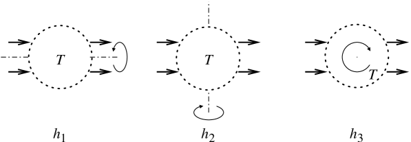
Figure 3.1: The half–turns $h_{1}$, $h_{2}$ and $h_{3}$

Let $h_{1}$, $h_{2}$ and $h_{3}$ be the half–turns about the indicated axes. Define three involutions $\rho_{1}$, $\rho_{2}$ and $\rho_{3}$ on the set of oriented $(2,2)$–tangles by $\rho_{1}T:=h_{1}(T)$, $\rho_{2}T:=-h_{2}(T)$ and $\rho_{3}T:=-h_{3}(T)$ (where $-h_{2}(T)$ and $-h_{3}(T)$ are the oriented $2$–tangles

Figure 3.2: The closure of the composition of $T_{1}$ and $T_{2}$

obtained from $h_{2}(T)$ and $h_{3}(T)$ by reversing the orientations of all strings). For two oriented (2,2)–tangles $T_{1}$ and $T_{2}$, denote by $T_{1}T_{2}$ the composition of $T_{1}$ and $T_{2}$ and by $(T_{1}T_{2})^{\wedge}$ the closure of $T_{1}T_{2}$ (see Figure 3.2).

Two oriented links $L$ and $L^{\prime}$ are called Conway mutants if there are two oriented $(2,2)$–tangles $T_{1}$ and $T_{2}$ such that for an involution $\rho_{i}$ $(i=1,2,3)$ the links $L$ and $L^{\prime}$ are respectively isotopic to $(T_{1}T_{2})^{\wedge}$ and $(T_{1}\rho_{i}T_{2})^{\wedge}$.

Theorem 6

Let $L$ and $L^{\prime}$ be Conway mutants. Then $L$ and $L^{\prime}$ are skein equivalent.

Proof. The proof goes by induction on the number $c$ of crossings of $T_{2}$. For $c\leq 1$, $T_{2}$ and $\rho_{i}T_{2}$ are isotopic, whence $L\sim L^{\prime}$. For $c>1$, modify a crossing of $T_{2}$ to obtain a skein triple of tangles $(T_{+},T_{-},T_{0})$ (with either $T_{+}=T_{2}$ or $T_{-}=T_{2}$, depending on whether the crossing is positive or negative). Denote by $(L_{+},L_{-},L_{0})$ and $(L^{\prime}_{+},L^{\prime}_{-},L^{\prime}_{0})$ the skein triples corresponding to $(T_{+},T_{-},T_{0})$ and $(\rho_{i}T_{+},\rho_{i}T_{-},\rho_{i}T_{0})$ respectively (i.e. $L_{+}=(T_{1}T_{+})^{\wedge}$, $L_{-}=(T_{1}T_{-})^{\wedge}$ and so on). By induction, $L_{0}\sim L^{\prime}_{0}$. Therefore, by the definition of skein equivalence, $L_{+}\sim L^{\prime}_{+}$ if and only if $L_{-}\sim L^{\prime}_{-}$. In other words, switching a crossing of $T_{2}$ does not affect the truth or falsity of the assertion. Since $T_{2}$ can be untied by switching crossings, we are back in the case $c\leq 1$. $\Box$

Corollary 1

The Jones polynomial is invariant under Conway mutation.

3.2 Mutation non–invariance of Khovanov homology

Let $P(L)$ denote the graded Poincaré polynomial of the complex $\mathcal{C}(L)$, i.e. let

$$P(L)(t,q):=\sum_{i,j}t^{i}q^{j}\dim_{\mathbb{Q}}(\mathcal{H}^{i,j}(L)\otimes\mathbb{Q})\;\in\mathbb{Z}[t^{\pm 1},q^{\pm 1}]\;.$$

By Theorem 4, we have $P(L)(-1,q)=J(L)(q)$, and by Corollary 1, $J(L)$ is invariant under Conway mutation. On the other hand, the following theorem gives examples of mutant links which are separated by $I(L)(t):=P(L)(t,1)$.

Theorem 7

Let $K_{i}$ $(i=1,2)$ be a $(2,n_{i})$ torus link, with $n_{i}>2$. Then the oriented links

$$L:=\bigcirc\sqcup(K_{1}\#K_{2})\\ \quad\text{and}\quad L^{\prime}:=K_{1}\sqcup K_{2}$$

are Conway mutants with $I(L)\neq I(L^{\prime})$. Here, $\bigcirc$ denotes the trivial knot and $K_{1}\#K_{2}$ is the connected sum of the oriented links $K_{1}$ and $K_{2}$. Note that the connected sum is well–defined even if $K_{i}$ has two components, because in this case the link $K_{i}$ is symmetric in its components.

Proof. From Figure 3.3 it is apparent that $L$ and $L^{\prime}$ are Conway mutants.

Figure 3.3: Figure : $L$ and $L^{\prime}$ are Conway mutants

The Khovanov complex of the trivial knot is

$$\ldots\hskip 6.50403pt\longrightarrow\hskip 6.50403pt0\hskip 6.50403pt\longrightarrow\hskip 6.50403pt0\hskip 6.50403pt\longrightarrow\hskip 6.50403ptA_{\operatorname{Kh}}\hskip 6.50403pt\longrightarrow\hskip 6.50403pt0\hskip 6.50403pt\longrightarrow\hskip 6.50403pt0\hskip 6.50403pt\longrightarrow\hskip 6.50403pt\ldots$$

Since $\operatorname{rank}(A_{\operatorname{Kh}})=2$, we get $I(\bigcirc)=2$, and since $P$ is multiplicative under disjoint union (see [Kh1, Proposition 33]), this implies $I(L)=2I(K_{1}\#K_{2})$. On the other hand, [Kh1, Proposition 35] tells us that

$$I(K_{i})=2+t^{-2}+t^{-3}+\ldots+t^{-(n_{i}-1)}+t^{-n_{i}}$$

for odd $n_{i}$, and

$$I(K_{i})=2+t^{-2}+t^{-3}+\ldots+t^{-(n_{i}-1)}+2t^{-n_{i}}$$

for even $n_{i}$. Since we assume $n_{i}>2$, we get that $I(K_{i})$ is not divisible by $2$. It follows that $I(L^{\prime})=I(K_{1})I(K_{2})$ is not divisible by $2$, and hence $I(L^{\prime})\neq I(L)$. $\Box$

Theorems 6 and 7 immediately imply:

Corollary 2

The skein equivalence class of a link does not determine its Khovanov homology. In particular, Khovanov homology is strictly stronger than the Jones polynomial.

Remark. Theorem 7 remains true if we allow $(2,n_{i})$ torus links $K_{i}$ with $n_{i}<-2$ (to see this, use [Kh1, Corollary 11], which relates the Khovanov homology of a link to the Khovanov homology of its mirror image). However, the condition $|n_{i}|>2$ is necessary. In fact, if one of the $|n_{i}|$ is $\leq 1$, then the corresponding torus link $K_{i}$ is trivial and hence $L$ and $L^{\prime}$ are isotopic. If one of the $|n_{i}|$, say $|n_{2}|$, is equal to $2$, then $K_{2}$ is a Hopf link and hence $L$ and $L^{\prime}$ are related to $\bigcirc\sqcup K_{1}$ by Hopf link addition (see Section 4.3). Now it follows from Theorem 9 (Section 4.3) that $\mathcal{H}^{i,j}(L)$ and $\mathcal{H}^{i,j}(L^{\prime})$ are both isomorphic to $\mathcal{H}^{i+2,j+5}(\bigcirc\sqcup K_{1})\oplus\mathcal{H}^{i,j+1}(\bigcirc\sqcup K_{1})$.

Remark. As yet, it is not known whether there are mutant knots ($1$–component links) with different Khovanov homology. An argument of D. Bar–Natan [B4], which would show invariance of Khovanov homology under knot mutation, was remarked to be incomplete by the author.

3.3 Computer Calculations with KhoHo

Tables 3.1 and 3.2 show the Khovanov homology of $L$ and $L^{\prime}$ for the case $n_{1}=n_{2}=3$. The tables where generated using A. Shumakovitch’s program KhoHo [S1]. The entry in the $i$–th column and the $j$–th row looks like $\hbox{$a$[$b$]}\over\lower 3.0pt\hbox{$c$}$, where $a$ is the rank of the homology group $\mathcal{H}^{i,j}$, $b$ the number of factors $\mathbb{Z}/2\mathbb{Z}$ in the decomposition of $\mathcal{H}^{i,j}$ into $p$–subgroups, and $c$ the rank of the chain group $\mathcal{H}^{i,j}$. The numbers above the horizontal arrows denote the ranks of the chain differentials.

In the examples, only $2$–torsion occurs. The reader may verify that not only the ranks but also the torsion parts of the $\mathcal{H}^{i,j}$ are different for $L$ and $L^{\prime}$. The ranks of $\mathcal{C}^{i,j}(L)$ and $\mathcal{C}^{i,j}(L^{\prime})$ agree because there is a natural one–to–one correspondence between the Kauffman states of $L$ and $L^{\prime}$.

 

    -6 -5 -4 -3 -2 -1 0

 

 

 

-2             $${\raise 1.0pt\hbox{\bf 1}\over\lower 3.0pt\hbox{\bf 1}}$$

             

 

       2      4      2

-4      

             

 

       1      5    10    18    13      5

-6  

             

 

       6    24    36    38    14      4

-8  

             

 

     15    45    44    28      5      1

-10  

             

 

     20    39    20      6

-12      

             

 

     15    13      2

-14        

             

 

       5

-16            

             

 

 

-18              

             

 

Table 3.1: Ranks of $\mathcal{H}^{i,j}$ and $\mathcal{C}^{i,j}$ and ranks of the differentials for the disjoint union of the unknot and the granny–knot

 

    -6 -5 -4 -3 -2 -1 0

 

 

 

-2             $${\raise 1.0pt\hbox{\bf 1}\over\lower 3.0pt\hbox{\bf 1}}$$

             

 

       2      4      2

-4      

             

 

       1      5    10    18    13      5

-6  

             

 

       6    24    36    38    14      4

-8  

             

 

     15    45    44    28      5      1

-10  

             

 

     20    40    20      6

-12      

             

 

     15    13      2

-14        

             

 

       6

-16            

             

 

 

-18              

             

 

Table 3.2: Ranks of $\mathcal{H}^{i,j}$ and $\mathcal{C}^{i,j}$ and ranks of the differentials for the disjoint union of two trefoil knots

Chapter 4 The spanning tree model

In [T], M. Thistlethwaite described a relation between the Kauffman bracket of a knot diagram $D$ and the Tutte polynomial of the Tait graph of $D$. He showed that the Kauffman bracket admits an expansion as a sum over terms corresponding to spanning trees of the Tait graph.

In [We2], the author constructed an analogue of this expansion for Khovanov homology. Independently, A. Champanerkar and I. Kofman [CK] proposed a similar construction, based on a technically different argument.

In this chapter, we first review the spanning tree expansion for the Kauffman bracket. Our approach is different from Thistlethwaite’s, making no explicit reference to the Tutte polynomial. In Section 4.2, we show how our ideas lead to a spanning tree model for the Khovanov bracket. In the remaining sections, we give several applications, among these a new proof of E. S. Lee’s [L1] theorem on the support of the Khovanov homology of alternating knots, and a short proof of a theorem on the behavior of the Khovanov bracket under Hopf link addition.

4.1 Spanning tree model for the Kauffman bracket

4.1.1 A simpler formula for the Kauffman bracket.

Suppose $D$ is an unoriented link diagram whose crossings are numbered. Recall that the Kauffman bracket of $D$ satisfies

$$\langle D\rangle=\sum_{D^{\prime}\in{\mathcal{K}}(D)}\langle D|D^{\prime}\rangle\langle D^{\prime}\rangle$$ (4.1)

where $\langle D|D^{\prime}\rangle=(-q)^{r(D,D^{\prime})}$. Formula (4.1) can be deduced recursively from the rule $\langle\slashoverback\rangle=\langle\smoothing\rangle-q\langle\hsmoothing\rangle$, as follows: first, we expand $\langle D\rangle$ as a sum of two terms by applying $\langle\slashoverback\rangle=\langle\smoothing\rangle-q\langle\hsmoothing\rangle$ to crossing number $1$. Next, we expand each these two terms by applying $\langle\slashoverback\rangle=\langle\smoothing\rangle-q\langle\hsmoothing\rangle$ to crossing number $2$. Continuing like this, we finally reach the Kauffman states and hence recover (4.1). The procedure is visualized in the binary tree below.

Figure 4.1: Binary tree used to deduce (4.1) from $\langle\slashoverback\rangle=\langle\smoothing\rangle-q\langle\hsmoothing\rangle$.

In case $D$ is connected, we can compute the Kauffman bracket of $D$ more efficiently, by modifying the above procedure as follows: as before, we successively expand terms by applying the relation $\langle\slashoverback\rangle=\langle\smoothing\rangle-q\langle\hsmoothing\rangle$ to the crossings. But before expanding a term, we check the connectivity of the two diagrams and appearing on the right–hand side of $\langle\slashoverback\rangle=\langle\smoothing\rangle-q\langle\hsmoothing\rangle$. If one of them is disconnected, we do not expand the crossing in the given term, and instead continue with the next crossing. The improved procedure is visualized in Figure 4.2.

Figure 4.2: Binary tree used to deduce (4.2).

The improved procedure leads to the expansion

$$\langle D\rangle=\sum_{D^{\prime}\in\mathcal{T}(D)}\langle D|D^{\prime}\rangle\langle D^{\prime}\rangle\;.$$ (4.2)

where $\mathcal{T}(D)$ denotes the set of all link diagrams sitting at the leaves of the tree in Figure. Note that $\mathcal{T}(D)$ depends on the numbering of the crossings of $D$.

To turn (4.2) into an explicit formula, we have to calculate the Kauffman brackets $\langle D^{\prime}\rangle$. Let $D^{\prime}$ be an element of $\mathcal{T}(D)$. By construction, $D^{\prime}$ is connected and every crossing of $D^{\prime}$ is splitting (i.e. connects two otherwise disconnected parts of $D^{\prime}$). Therefore, $D^{\prime}$ represents the unknot and it can be transformed into the trivial diagram using Reidemeister move R1 only. We call a diagram with this property R1–trivial. After orienting $D^{\prime}$ arbitrarily, we get $J(D^{\prime})=J(\bigcirc)=q+q^{-1}$ and hence

$$\langle D^{\prime}\rangle=(-1)^{c_{-}(D^{\prime})}q^{2c_{-}(D^{\prime})-c_{+}(D^{\prime})}(q+q^{-1})\;.$$ (4.3)

Inserting (4.3) into (4.2), we obtain

$$\langle D\rangle=\sum_{D^{\prime}\in\mathcal{T}(D)}(-q)^{r(D,D^{\prime})}(-1)^{c_{-}(D^{\prime})}q^{2c_{-}(D^{\prime})-c_{+}(D^{\prime})}(q+q^{-1})\;.$$ (4.4)

Note that the set of Kauffman states ${\mathcal{K}}(D)$ is the disjoint union of all sets ${\mathcal{K}}(D^{\prime})$, for all $D^{\prime}\in\mathcal{T}(D)$. We construct a map

$$\begin{array}[]{ccc}{\mathcal{K}}(D)&\longrightarrow&\mathcal{T}(D)\\ S&\longmapsto&D_{S}\end{array}$$

by defining $D_{S}$ to be the unique element of $\mathcal{T}(D)$ satisfying $S\in{\mathcal{K}}(D_{S})$. Let ${\mathcal{K}}_{1}(D)\subset{\mathcal{K}}(D)$ denote the set of all Kauffman states which consist of exactly one circle. When restricted to ${\mathcal{K}}_{1}(D)\subset{\mathcal{K}}(D)$, the above map becomes a bijection. Indeed, since $D^{\prime}\in\mathcal{T}(D)$ is R1–trivial, we have $\#{\mathcal{K}}_{1}(D^{\prime})=1$ and hence $D^{\prime}$ has a unique preimage in ${\mathcal{K}}_{1}(D)$.

We may rewrite (4.2) as

$$\langle D\rangle=\sum_{S\in{\mathcal{K}}_{1}(D)}\langle D|D_{S}\rangle\langle D_{S}\rangle.$$ (4.5)

Formula (4.4) becomes

$$\begin{split}\langle D\rangle&=\sum_{S\in{\mathcal{K}}_{1}(D)}(-q)^{r(D,D_{S})}(-1)^{c_{-}(D_{S})}q^{2c_{-}(D_{S})-c_{+}(D_{S})}(q+q^{-1})\\ &=\sum_{S\in{\mathcal{K}}_{1}(D)}(-1)^{r(D,S)-w(D_{S})}q^{r(D,S)-2w(D_{S})}(q+q^{-1})\end{split}$$ (4.6)

where the second equality follows by observing that $r(D,D_{S})=r(D,S)-r(D_{S},S)=r(D,S)-c_{+}(D_{S})$ and by writing $w(D_{S})$ for $c_{+}(D_{S})-c_{-}(D_{S})$.

4.1.2 The relation with spanning trees.

Assume that the regions of $D$ are colored black and white in a checkerboard fashion, such that any two neighbored regions have opposite colors, and such that the unbounded region is colored white. The Tait graph $\Gamma_{D}$ is the planar graph whose vertices are the black regions and whose edges correspond to the crossings of $D$ (see Figure 4.3).

Figure 4.3: The Tait graph.

Given a smoothing of a crossing of $D$, we call it a black or a white smoothing depending on whether it connects black or white regions of $D$.

Let $\mathcal{T}(\Gamma_{D})$ denote the set of all spanning trees of $\Gamma_{D}$. There is a bijection

$$\begin{array}[]{ccc}\mathcal{T}(\Gamma_{D})&\longrightarrow&{\mathcal{K}}_{1}(D)\\ T&\longmapsto&S_{T}\end{array}$$

defined as follows: to a tree $T$ we associate the connected Kauffman state $S_{T}$ obtained by choosing the black smoothing for precisely those crossings which correspond to an edge of $T$, and the white smoothing for all other crossings. Using the above bijection, we can can rewrite formula (4.5) as

$$\langle D\rangle=\sum_{T\in\mathcal{T}(\Gamma_{D})}\langle D|D_{T}\rangle\langle D_{T}\rangle$$

where we have abbreviated $D_{T}$ for $D_{S_{T}}$.

The correspondence between spanning trees and elements of ${\mathcal{K}}_{1}(D)$ leads to an easy proof of the following lemma.

Lemma 8

The number of black smoothings is the same in all $S\in{\mathcal{K}}_{1}(D)$.

Proof. Since black smoothings in $S_{T}$ correspond to edges of $T$, it suffices to show that all spanning trees of $\Gamma_{D}$ have the same number of edges. But this is obvious, because the number of edges in any spanning tree is just one less than the number of vertices of $\Gamma_{D}$. $\Box$ An alternative proof of Lemma 8 uses Kauffman’s Clock Theorem [Ka1]. By the Clock Theorem, any two elements of ${\mathcal{K}}_{1}(D)$ are related by a finite sequence of state transpositions (see Figure 4.4). The lemma follows because state transpositions do not change the number of black smoothings.

Of course, the lemma also implies that the number of white smoothings is the same in all $S\in{\mathcal{K}}_{1}(D)$.

Figure 4.4: A knot projection, and two smoothings related by a state transposition.

4.2 Spanning tree model for the Khovanov bracket

In this section, we discuss how the construction of Section 4.1 transfers to the formal Khovanov bracket. The main result is stated in the following theorem.

Theorem 8

Let $D$ be a connected link diagram. Then the formal Khovanov bracket $\left[\!\!\left[D\right]\!\!\right]$ destabilizes to a subcomplex $ST(D)$. On the level of objects (i.e. if one ignores the differential), $ST(D)$ is isomorphic to

$$ST(D)\cong\bigoplus_{S\in{\mathcal{K}}_{1}(D)}U[r(D,S)-w(D_{S})]\{r(D,S)-2w(D_{S})\}$$ (4.7)

where $U:=\left[\!\!\left[\bigcirc\right]\!\!\right]$ denotes the formal Khovanov bracket of the trivial diagram consisting of a single circle. We call $ST(D)$ the spanning tree subcomplex of $\left[\!\!\left[D\right]\!\!\right]$.

Theorem 8 can be viewed as a “categorification” of formula (4.6). Indeed, since $U\cong\emptyset\{1\}\oplus\emptyset\{-1\}$ by Lemma 3, the shifts of the gradings in (4.7) agree with the powers of $-1$ and $q$ in (4.6). Before proving the theorem, we mention two corollaries.

Corollary 3

Let $D$ be a connected link diagram. Then $\overline{\mathcal{C}}(D)$ destabilizes to the subcomplex $\mathcal{F}_{\operatorname{Kh}}(ST(D))\subset\overline{\mathcal{C}}(D)$. As a bigraded module, $\mathcal{F}_{\operatorname{Kh}}(ST(D))$ is isomorphic to

$$\mathcal{F}_{\operatorname{Kh}}(ST(D))\cong\bigoplus_{S\in{\mathcal{K}}_{1}(D)}A_{\operatorname{Kh}}[r(D,S)-w(D_{S})]\{r(D,S)-2w(D_{S})\}\;.$$

$\mathcal{F}_{\operatorname{Kh}}(ST(D))$ will be called the spanning tree subcomplex of $\overline{\mathcal{C}}(D)$.

Using that $A_{\operatorname{Kh}}=\mathbb{Z}{\bf 1}\oplus\mathbb{Z}X$ and $\deg({\bf 1})=+1$ and $\deg(X)=-1$, we get the following estimate for the ranks of the Khovanov homology groups:

Corollary 4

Let $D$ be a connected link diagram. Then

$$\dim_{\mathbb{Q}}(\overline{\mathcal{H}}(D)\otimes\mathbb{Q})\leq 2(\#{\mathcal{K}}_{1}(D))\;.$$

Moreover, the rank of $\overline{\mathcal{H}}^{i,j}(D)$ is bounded from above by the number of $S\in{\mathcal{K}}_{1}(D)$ with $r(D,S)-w(D_{S})=i$ and $r(D,S)=2i-j\pm 1$.

Corallary 4 shows that the ranks of the homology groups $\overline{\mathcal{H}}^{i,j}(D)$ tend to be much smaller than the ranks of the chain groups $\overline{\mathcal{C}}^{i,j}(D)$. This is consistent with Bar–Natan’s experimental observation [B1].

Proof of Theorem 8. To prove the theorem, we reformulate the arguments which led us to formula (4.6) in Section 4.1 in the setting of the formal Khovanov bracket.

First, we consider a diagram $D^{\prime}\in\mathcal{T}(D)$ sitting at a leaf of the binary tree of Figure 4.2. Since $D^{\prime}$ is R1–trivial, part 1 of Lemma 4 (Subsection 1.3.5) implies that $\left[\!\!\left[D^{\prime}\right]\!\!\right]$ destabilizes to a subcomplex isomorphic to $U[c_{-}(D^{\prime})]\{2c_{-}(D^{\prime})-c_{+}(D^{\prime})\}$. Comparing this with (4.3), we see that the theorem is true for the diagrams sitting at the leaves of the tree.

Now we proceed inductively, going up the tree. Let $D_{1}$ be a diagram sitting at an internal node of the tree, and let $D_{2}$ and $D_{3}$ be the two diagrams sitting right below that node. By induction, the complexes $\left[\!\!\left[D_{2}\right]\!\!\right]$ and $\left[\!\!\left[D_{3}\right]\!\!\right]$ destabilize to subcomplexes $ST(D_{2})$ and $ST(D_{3})$. Moreover, $\left[\!\!\left[D_{1}\right]\!\!\right]$ is isomorphic to the mapping cone of a chain transformation between $\left[\!\!\left[D_{2}\right]\!\!\right]$ and $\left[\!\!\left[D_{3}\right]\!\!\right]\{1\}$ (see (1.11)). By Lemma 2 (Subsection 1.3.1), forming the mapping cone “commutes” with destabilization. Therefore, $\left[\!\!\left[D_{1}\right]\!\!\right]$ destabilizes to a subcomplex $ST(D_{1})$ which is isomorphic to the mapping cone of a chain transformation between $ST(D_{2})$ and $ST(D_{3})\{1\}$. In particular, on the level of objects we have $ST(D_{1})\cong ST(D_{2})\oplus ST(D_{3})\{1\}[1]$. Using this as a substitute for the relation $\langle D_{1}\rangle=\langle D_{2}\rangle-q\langle D_{3}\rangle$, and arguing as in Section 4.1, we get the theorem. $\Box$

Remark. Let $D$ be a link diagram. After selecting a point $P$ on an edge of $D$, we can endow $\overline{\mathcal{C}}(D)$ with the structure of an $A_{\operatorname{Kh}}$–module, as follows: multiplication by ${\bf 1}\in A_{\operatorname{Kh}}$ is the identity map; multiplication by $X\in A_{\operatorname{Kh}}$ is induced by “multiplying” with a dot at point $P$. The reduced Khovanov complexes are the complexes $\overline{\mathcal{C}}(D)\otimes_{A_{\operatorname{Kh}}}\mathbb{Z}X$ and $\overline{\mathcal{C}}(D)\otimes_{A_{\operatorname{Kh}}}(A_{\operatorname{Kh}}/\mathbb{Z}X)$, where $\mathbb{Z}X\subset A_{\operatorname{Kh}}$ denotes the $A_{\operatorname{Kh}}$–submodule of $A_{\operatorname{Kh}}$ generated by $X\in A_{\operatorname{Kh}}$. If one performs the R1 moves in the proof of Theorem 8 far away from $P$, the isomorphism in Corollary 3 becomes an isomorphism of $A_{\operatorname{Kh}}$–modules. By tensoring with $\mathbb{Z}X$ and $A_{\operatorname{Kh}}/\mathbb{Z}X$, one gets spanning tree models for the reduced Khovanov complexes.

Remark. Spanning trees of the Tait graph also appear as generators of the knot Floer complex [OS1]. Hence the spanning tree model might shed some light on the relation between Khovanov homology and knot Floer homology.

4.3 Hopf link addition

In this section, we apply the spanning tree model to prove a theorem, which was originally proved (for Khovanov homology) by M. Asaeda and J. Przytycki [AP]. As mentioned in [We1], the theorem also follows from [Kh1, Corollary 10].

Theorem 9

Assume the link diagram $D\#H$ is obtained from a link diagram $D$ by Hopf link addition (see Figure 4.5). Then the complex $\left[\!\!\left[D\#H\right]\!\!\right]$ destabilizes to the direct sum $\left[\!\!\left[D\right]\!\!\right][0]\{-1\}\oplus\left[\!\!\left[D\right]\!\!\right][2]\{3\}$.

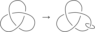
Figure 4.5: Hopf link addition.

To prove the theorem, we observe that the spanning tree model extends to $(1,1)$–tangles, i.e. tangles having exactly two boundary points, as in Figure 4.6. The only difference is that the Tait graph of a $(1,1)$–tangle has a distinguished vertex (the vertex which corresponds to the black region adjacent to the dotted circle), and hence the spanning trees are rooted.

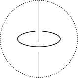
Figure 4.6: A $(1,1)$–tangle.

Let $H^{\prime}$ denote the $(1,1)$–tangle shown in Figure 4.6. Inserting $H^{\prime}$ into an edge of $D$ has the same effect as summing a Hopf link to that edge of $D$. The Tait graph of $H^{\prime}$ has exactly two spanning trees.

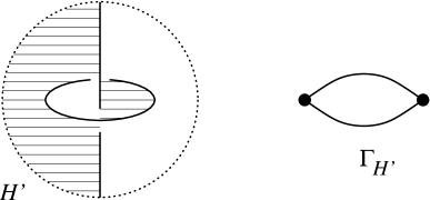
Figure 4.7: Tait graph of $H^{\prime}$.

Now the spanning tree model tells us that $\left[\!\!\left[H^{\prime}\right]\!\!\right]$ destabilizes to a subcomplex $ST(H^{\prime})$, which is isomorphic on the level of objects to $\left[\!\!\left[\;|\;\right]\!\!\right][0]\{-1\}\oplus\left[\!\!\left[\;|\;\right]\!\!\right][2]\{3\}$. Here “$\,|\,$” denotes the trivial $(1,1)$–tangle, consisting of a single vertical line. Note that the homological gradings of the two summands in $\left[\!\!\left[\;|\;\right]\!\!\right][0]\{-1\}\oplus\left[\!\!\left[\;|\;\right]\!\!\right][2]\{3\}$ differ by two. Therefore, $ST(H^{\prime})$ must have trivial differential, and so the isomorphism $ST(H^{\prime})\cong\left[\!\!\left[\;|\;\right]\!\!\right][0]\{-1\}\oplus\left[\!\!\left[\;|\;\right]\!\!\right][2]\{3\}$ is actually an isomorphism of complexes. Using the good composition properties of the Khovanov bracket with respect to gluing of tangles, we get the theorem.

4.4 Alternating knots

The theorems in this section were conjectured by D. Bar–Natan, S. Garoufalidis and M. Khovanov [B1] and proved by E. S. Lee [L1]. We give new proofs using the spanning tree model. For short proofs, see also [AP].

A knot diagram is said to be alternating if one alternately over– and undercrosses other strands as one goes along the knot in that diagram. A knot is called alternating if it possesses an alternating diagram.

Lemma 9

Let $D$ be an alternating knot diagram. Then the number of $1$–smoothings in $S$ is the same for all $S\in{\mathcal{K}}_{1}(D)$.

Proof. Since $D$ is alternating, we necessarily have one of the following two situations: either the $1$–smoothings coincide with the black smoothings, or the $1$–smoothings coincide with the white smoothings. Hence Lemma 9 follows from Lemma 8 of Subsection 4.1.2. $\Box$

Given an an alternating knot diagram $D$, we denote by $n_{1}(D):=r(D,S)$ the number of $1$–smoothings in any $S\in{\mathcal{K}}_{1}(D)$. Corollary 4 implies:

Theorem 10

Let $D$ be an alternating knot diagram. $\overline{\mathcal{H}}^{i,j}(D)$ is zero unless the pair $(i,j)\in\mathbb{Z}^{2}$ lies on one of the two lines $j=2i-n_{1}(D)\pm 1$.

Let $i_{-}$ and $i_{+}$ denote the smallest and largest integer $i$ for which there is an $S\in{\mathcal{K}}_{1}(D)$ such that $r(D,S)-w(D_{S})=i$. Let $j_{-}:=2i_{-}-n_{1}(D)-1$ and $j_{+}:=2i_{+}-n_{1}(D)+1$.

Since the spanning tree subcomplex $\mathcal{F}_{\operatorname{Kh}}(ST(D))$ of an alternating knot diagram $D$ is concentrated on the two lines $j=2i-n_{1}(D)\pm 1$, and since the differential has bidegree $(1,0)$, we get the following theorem.

Theorem 11

Let $D$ be an alternating knot diagram. Then

1. $\overline{\mathcal{H}}^{i,j}(D)$ is zero unless $i_{-}\leq i\leq i_{+}$.

2. $\overline{\mathcal{H}}^{i,j}(D)$ is torsion free unless $j=2i-n_{1}(D)-1$.

3. $\overline{\mathcal{H}}^{i_{-},j_{-}}(D)$ and $\overline{\mathcal{H}}^{i_{+},j_{+}}(D)$ are non–zero and torsion free.

Recall that a crossing of $D$ is called splitting if it connects two otherwise disconnected parts of $D$.

Theorem 12

Let $D$ be an alternating knot diagram with $c$ crossings. Assume that no crossing of $D$ is splitting. Then $\overline{\mathcal{H}}^{i_{-},j_{-}}(D)=\overline{\mathcal{H}}^{i_{+},j_{+}}(D)=\mathbb{Z}$. Moreover, $i_{-}=0$ and $i_{+}=c$.

Proof. By part 3 of the previous theorem, we know that $\overline{\mathcal{H}}^{i_{-},j_{-}}(D)$ and $\overline{\mathcal{H}}^{i_{+},j_{+}}(D)$ are free abelian groups of rank at least one. To show that the rank is exactly one, it suffices to show that there is only one $S\in{\mathcal{K}}_{1}(D)$ contributing to the lowest degree $i_{-}$, i.e. such that $r(D,S)-w(D_{S})=i_{-}$, and likewise only one $S\in{\mathcal{K}}_{1}(D)$ contributing to the highest degree $i_{+}$, i.e. such that $r(D,S)-w(D_{S})=i_{+}$.

Actually, we prove something slightly different. Recall that the spanning tree construction depends on a numbering of the crossings of $D$. In particular, the diagram $D_{S}$ associated to $S\in{\mathcal{K}}_{1}(D)$ depends on the numbering of the crossings. What we show is that for any $S\in{\mathcal{K}}_{1}(D)$, there exists a numbering such that $S$ is the unique state contributing to lowest/highest degree. This is the content of the following lemma. $\Box$

Lemma 10

Let $D$ be an alternating knot diagram with $c$ crossings, all of which are non–splitting, and let $S$ be an element of ${\mathcal{K}}_{1}(D)$.

1. There is a numbering of the crossings of $D$ such that $-w(D_{S})=-n_{1}(D)$, and $-w(D_{S^{\prime}})>-n_{1}(D)$ for all $S^{\prime}\in{\mathcal{K}}_{1}(D)$ with $S^{\prime}\neq S$.

2. Likewise, there is a numbering of the crossings of $D$ such that $-w(D_{S})=c-n_{1}(D)$, and $-w(D_{S^{\prime}})<c-n_{1}(D)$ for all $S^{\prime}\in{\mathcal{K}}_{1}(D)$ with $S^{\prime}\neq S$.

Proof. 1. Let $S$ be an element of ${\mathcal{K}}_{1}(D)$. Assume that the crossings of $D$ are numbered in such a way that the crossings which are $0$–smoothings in $S$ precede those which are $1$–smoothings in $S$. We claim that for this numbering, the relations in part 1 of Lemma 10 are satisfied, i.e. $-w(D_{S})=-n_{1}(D)$, and $-w(D_{S^{\prime}})>-n_{1}(D)$ for all $S^{\prime}\in{\mathcal{K}}_{1}(D)$ with $S^{\prime}\neq S$.

To see this, we consider the link diagrams $D_{k}$, $0\leq k\leq c-n_{1}(D)$, obtained from $D$ by replacing the first $k$ crossings of $D$ by their $0$–smoothings, while leaving the remaining $c-k$ crossings unchanged. We denote by $D^{\prime}$ the diagram $D^{\prime}:=D_{c-n_{1}(D)}$. Note that if one replaces all crossings in $D^{\prime}$ by their $1$–smoothings, the result is the state $S$. Since $S$ is connected, so is $D^{\prime}$, and so are all $D_{k}$ with $k\leq c-n_{1}(D)$.

Because $D$ is alternating, we may assume without loss of generality that the $1$–smoothings in $S$ are the black smoothings, and hence correspond to the edges of the spanning tree associated to $S$. Using that every edge in a tree connects two otherwise disconnected parts, we get that every crossing of $D^{\prime}$ is splitting, i.e. connects to otherwise disconnected parts of $D^{\prime}$.

Claim. $D_{S}=D^{\prime}$. Proof of the claim. Recall the binary tree of Figure 4.2, which was used to deduce the spanning tree expansion. If at all $D^{\prime}$ appears in this tree, then the afore mentioned properties of $D^{\prime}$ imply that it must be the leaf $D_{S}$.

Thus, it suffices show that the sequence $D=D_{0},D_{1},\ldots,D_{c-n_{1}(D)}=D^{\prime}$ appears along a path going down the binary tree. Since $D_{k+1}$ results from $D_{k}$ by resolving the first crossing of $D_{k}$, we only have to check that for all $k<c-n_{1}(D)$ the first crossing of $D_{k}$ is non–splitting. This can be done by observing that the last $n_{1}(D)$ crossings of $D_{k}$ form the edges of a spanning tree (same argument as used above for $D^{\prime}$), and using that the Tait graph of $D$ is loop–less because all crossings of $D$ are non–splitting. We leave the details to the reader. $\Box$

So we have that $D_{S}=D^{\prime}$, and we also know that the (unsmoothened) crossings in $D^{\prime}$ are the $1$–smoothings in $S$. Since $D_{S}$ is connected and since all of its crossings are splitting, this implies that all crossings of $D_{S}$ must be positive with respect to an arbitrary orientation of $D_{S}$. We conclude $w(D_{S})=c_{+}(D_{S})=n_{1}(D)$.

Now consider $S^{\prime}\in{\mathcal{K}}_{1}(D)$ with $S^{\prime}\neq S$. Recall that $S$ and $S^{\prime}$ both have exactly $n_{1}(D)$ $1$–smoothings. In $S$ the $1$–smoothings come after the $0$–smoothings. Therefore, the first crossing of $D$ where $S$ and $S^{\prime}$ differ has to be a $0$–smoothing in $S$ and a $1$–smoothing in $S^{\prime}$. Being a $0$–smoothing in $S$, this crossing is smoothened in $D_{S}=D^{\prime}$. We leave it to the reader to conclude that it also has to be smoothened in $D_{S^{\prime}}$. Thus we have found a $1$–smoothing in $S^{\prime}$ which is smoothened in $D_{S^{\prime}}$. This implies $c_{+}(D_{S^{\prime}})<n_{1}(D)$ (cf. previous paragraph) and hence $-w(D_{S^{\prime}})\geq-c_{+}(D_{S^{\prime}})>-n_{1}(D)$.

2. The second part of the lemma is proved analogously, by numbering the crossings of $D$ in such a way that the crossings which are $1$–smoothings in $S$ precede those which are $0$–smoothings in $S$. $\Box$

The above proof was inspired by [T]. For a different proof of a similar statement, see [Kh1, Section 7.7].

Corollary 5

If a knot possesses an alternating diagram with $c$ crossings, all of which are non–splitting, then the knot does not admit a diagram with fewer than $c$ crossings.

Proof. By part 1 of Theorem 11, $i_{+}(D)$ and $i_{-}(D)$ are equal to the highest and the lowest homological degree in which $\overline{\mathcal{H}}(D)$ is non–zero. Therefore, the difference $i_{+}(D)-i_{-}(D)$ is a lower bound for the number of crossings of $D$. Moreover, $i_{+}(D)-i_{-}(D)$ is a knot invariant. Now assume that $D$ is an alternating diagram with $c$ crossings, all of which are non–splitting. By Theorem 12, we have $i_{+}(D)-i_{-}(D)=c$, and hence the corollary follows. $\Box$

Remark. For alternating knots, the spanning tree model allows to calculate the reduced Khovanov homology completely. Indeed, for an alternating knot the reduced spanning tree subcomplex is supported on a single line $j=2i+const$ in the $ij$–plane. Since the differential has bidegree $(1,0)$, it must vanish. Therefore, the reduced spanning tree subcomplex is isomorphic to the reduced Khovanov homology of the alternating knot.

Remark. We can also consider the subcomplex $\mathcal{F}_{\operatorname{Lee}}(ST(D))\subset\mathcal{C}^{\prime}(D)$. While we know explicit generators for Lee homology from Section 2.1, the spanning tree description of Lee’s complex has the advantage that it also makes a statement about the filtration, and that it works well for Lee homology over $\mathbb{Z}$ coefficients. Theorem 10 and part 1 of Theorem 11 remain valid for Lee homology. Example. Let $D$ be a standard diagram of the left handed trefoil. Let $\mathcal{F}^{\mathbb{Z}}_{\operatorname{Lee}}$ denote Lee’s functor with $\mathbb{Z}$ coefficients, and let $A^{\mathbb{Z}}_{\operatorname{Lee}}:=\mathcal{F}^{\mathbb{Z}}_{\operatorname{Lee}}(\bigcirc)$ (so $A^{\mathbb{Z}}_{\operatorname{Lee}}=A_{\operatorname{Kh}}$, except that $A^{\mathbb{Z}}_{\operatorname{Lee}}$ is filtered whereas $A_{\operatorname{Kh}}$ is graded). We have

$$\mathcal{F}^{\mathbb{Z}}_{\operatorname{Lee}}(ST(D))\cong A^{\mathbb{Z}}_{\operatorname{Lee}}[0]\{-1\}\oplus A^{\mathbb{Z}}_{\operatorname{Lee}}[2]\{3\}\oplus A^{\mathbb{Z}}_{\operatorname{Lee}}[3]\{5\}$$

The differential is zero on $A^{\mathbb{Z}}_{\operatorname{Lee}}[0]\{-1\}$, and it maps ${\bf 1},X\in A^{\mathbb{Z}}_{\operatorname{Lee}}[2]\{3\}$ to $2X,2\cdot{\bf 1}\in A^{\mathbb{Z}}_{\operatorname{Lee}}[3]\{5\}$. Hence

$$\mathcal{H}^{\prime}(D;\mathbb{Z})\cong A^{\mathbb{Z}}_{\operatorname{Lee}}[0]\{-1\}\oplus(A^{\mathbb{Z}}_{\operatorname{Lee}}/2A^{\mathbb{Z}}_{\operatorname{Lee}})[3]\{5\}$$

Note that there is $2$–torsion in bidegree $(3,6)$, despite the fact that the pair $(3,6)$ lies on the upper of the two lines mentioned in Theorem 10, and despite the fact that $(3,6)=(i_{+},j_{+})$. Hence parts 2 and 3 of Theorem 11 do not transfer to Lee homology with $\mathbb{Z}$ coefficients.

Chapter 5 Framed link cobordisms

In this chapter, we introduce movie presentations and movie moves for framed link cobordisms.

5.1 Framed links

Let $L\subset\mathbb{R}^{3}$ be a link. A framing of $L$ is a homotopy class of trivializations of the normal bundle of $L$ in $\mathbb{R}^{3}$. Equivalently, a framing can be defined as homotopy class of non–singular normal vector fields on $L$. A link equipped with a framing is called a framed link.

Let $K\subset\mathbb{R}^{3}$ be a knot and let $f$ be a framing of $K$. Represent $f$ by a non–singular normal vector field, and assume that the vectors are sufficiently short, so that their tips trace out a knot $K^{\prime}$ parallel to $K$. The framing coefficient of $f$ is the linking number $n(f):=\operatorname{lk}(K,K^{\prime})$ of $K$ and $K^{\prime}$. One can show that $f$ is completely determined by its framing coefficient $n(f)$.

If $L$ is a link, a framing of $L$ can be specified by specifying a framing $f_{i}$ for each component $L_{i}$ of $L$. The total framing coefficient of $L$ is defined by

$$n(f):=\sum_{i}n(f_{i})+2\sum_{i<j}\operatorname{lk}(L_{i},L_{j})\;.$$

There are several methods for describing framed links. One possibility is to take an ordinary link diagram $D$ and then think of it as presenting a framed link, framed by the blackboard framing, i.e. by the framing which is given by a vector field which is everywhere parallel to the plane of the picture.

Figure 5.1: The blackboard framing.

It is easy to see that the framing coefficient of the blackboard framing is equal to the writhe of $D$. Since the writhe changes by $\pm 1$ under move R1, the blackboard framing is not invariant under this move. However, it is invariant under the move FR1 shown in Figure 5.2. In fact, if one uses the blackboard framing to present framed links, then two link diagrams represent isotopic framed links if and only if they are related by a finite sequence of the moves FR1, R2 and R3.

Figure 5.2: The framed Reidemeister move FR1.

Another way of presenting framed links uses link diagrams with signed points. A link diagram with signed points is a link diagram $D$, together with a finite collection of distinct points, lying on the interiors of the edges of $D$, and labelled by $+$ or $-$. Such a diagram presents a framed link, with framing $f_{D}$ given as follows: $f_{D}$ is represented by a vector field which is everywhere parallel to the drawing plane, except in a small neighborhood of the signed points, where it winds around the link, in such a way that each positive point contributes $+1$ to $n(f_{D})$ and each negative point contributes $-1$. Note that $n(f_{D})=w(D)+t(D)$, where $t(D)$ denotes the difference between the numbers of positive and negative signed points in $D$.

Figure 5.3: The signed Reidemeister move SR1.

The signed first Reidemeister move SR1, shown above, leaves $n(f_{D})$ unchanged. It follows that two link diagrams with signed points describe isotopic framed links if and only if they are related by a finite sequence of the following moves: the moves SR1, R2 and R3, as well as creation/annihilation of pairs of nearby oppositely signed points, and sliding signed points past crossings.

The $m$–cable of a framed knot $K$ is the $m$–component link $K^{m}$, obtained by replacing $K$ by $m$ parallel strands, pushed off in the direction of the framing vector field.

Figure 5.4: $3$–cable of a framed knot (framed by the blackboard framing).

5.2 Framings on submanifolds of codimension $2$

The concept of framings is not restricted to links. In this section, we study framings on arbitrary submanifolds of codimension $2$.

Let $M$ be a smooth oriented $(n+2)$–manifold and let $N\subset M$ be a smooth oriented compact submanifold of $M$ of dimension $n$. A framing of $N$ is a homotopy class of trivialization of the normal bundle $\nu_{N}$ of $N\subset M$. If $N$ has non–empty boundary and a trivialization $t$ of $\nu_{N}|_{\partial N}$ is specified, we define a relative framing of $N$ (relative to $t$) as a homotopy class of trivializations of $\nu_{N}$ which agree with $t$ over $\partial N$.

Lemma 11

Let $t$ be a trivialization of $\nu_{N}|_{\partial N}$. If non–empty, the set of relative framings of $N$ (relative to $t$) is an affine space over $H_{n-1}(N)$.

Proof. Since $\nu_{N}$ is an oriented $2$–plane bundle, its structural group is $SO(2)$. Therefore the difference between two relative framings is given by a homotopy class of maps from the pair $(N,\partial N)$ to the pair $(SO(2),1)$, i.e. by an element of $[N,\partial N;SO(2),1]$. Using that $SO(2)$ is a $K(\mathbb{Z},1)$ space, we can identify $[N,\partial N;SO(2),1]$ with $H^{1}(N,\partial N)$. And by Poincaré duality, $H^{1}(N,\partial N)$ is isomorphic to $H_{n-1}(N)$. $\Box$

Let us consider pairs $(E,t)$ where $E$ is an oriented $2$–plane bundle over $N$, and $t$ is a trivialization of $E|_{\partial N}$. We call two such pairs $(E,t)$ and $(E^{\prime},t^{\prime})$ isomorphic if there is an isomorphism $F:E\rightarrow E^{\prime}$ of oriented $2$–plane bundles such that $t^{\prime}\circ F=t$ over $\partial N$.

Lemma 12

Isomorphism classes of pairs $(E,t)$ correspond bijectively to elements of $H_{n-2}(N)$.

Proof. Isomorphism classes of pairs $(E,t)$ are classified by homotopy classes of maps from the pair $(N,\partial N)$ to the pair $(BSO(2),p_{0})$, where $p_{0}\in BSO(2)$ is an arbitrary basepoint. Since $BSO(2)$ is a $K(\mathbb{Z},2)$ space, we obtain $[N,\partial N;BSO(2),p_{0}]=H^{2}(N,\partial N)=H_{n-2}(N)$. $\Box$

Let $e(E,t)\in H_{n-2}(N)$ denote the homology class corresponding to the pair $(E,t)$. We immediately obtain:

Lemma 13

$N$ admits a framing (relative to $t$) if and only if $e(\nu_{N},t)=0$.

We are mainly interested in the case where $N$ is a connected surface $S$, embedded in a $4$–manifold $M$. In this case, $e(\nu_{S},t)$ is an integer $e(\nu_{S},t)\in H_{0}(S)=\mathbb{Z}$ which can be described as follows: identify $S$ with the zero section of $\nu_{S}$, and consider a section $S^{\prime}$ of $\nu_{S}$, whose restriction to the boundary $\partial S$ is non–vanishing and constant with respect to the trivialization $t$. Then $e(\nu_{S},t)=S\cdot S^{\prime}$ where $S\cdot S^{\prime}$ denotes the algebraic intersection number of the surfaces $S$ and $S^{\prime}$ in the total space of $\nu_{S}$. Since $S$ has a tubular neighborhood in $M$ which is diffeomorphic to the total space of $\nu_{S}$, we can view $e(\nu_{S},t)$ as a relative self–intersection number of $S$ in $M$.

Now assume $e(\nu_{S},t)=0$. Then the set of relative framings on $S$ is non–empty and hence an affine space over $H_{1}(S)$ (by Lemma 11). The action of $H_{1}(S)$ on framings can be described as follows. Let $c$ be an oriented simple closed curve on $S$ representing an element of $H_{1}(S)$. Consider a tubular neighborhood $U\subset S$ of $c$, diffeomorphic to $c\times[0,2\pi]$. Let $\chi_{c}$ be the map from $S$ to $SO(2)$ which is trivial on the complement of $U$ and maps a point $(\theta,\varphi)\in U=c\times[0,2\pi]$ to rotation by $\varphi$. Now $[c]$ acts on framings by sending the framing given by a vector field $v(z)$ to the framing given by the vector field $\chi_{c}(z)v(z)$. Note that the Poincaré dual $\operatorname{PD}^{-1}[c]\in H^{1}(S,\partial S)$ has the following interpretation: let $c^{\prime}$ be a properly embedded simple curve on $S$ representing an element of $H_{1}(S,\partial S)$. The restriction $\chi_{c}|_{c^{\prime}}$ is a closed curve in $SO(2)$, which winds around $SO(2)$ once at every intersection point of $c^{\prime}$ with $c$. Hence the class of $\chi_{c}|_{c^{\prime}}$ in $\pi_{1}(SO(2),1)=\mathbb{Z}$ is given by $[\chi_{c}|_{c^{\prime}}]=c\cdot c^{\prime}=\langle\operatorname{PD}^{-1}[c],[c^{\prime}]\rangle$.

5.3 Framed link cobordisms

Now let $S\subset\mathbb{R}^{3}\times[0,1]$ be a connected link cobordism between two oriented framed links $L_{0}$ and $L_{1}$.

Lemma 14

$S$ admits a relative framing, relative to the given framings of $L_{0}$ and $L_{1}$, if and only if the total framing coefficients of $L_{0}$ and $L_{1}$ agree.

Proof. For the sake of simplicity, we restrict to the case where $S$ is a cobordism between knots $K_{0}$ and $K_{1}$. Let $K_{0}^{\prime}$ and $K_{1}^{\prime}$ be parallels of $K_{0}$ and $K_{1}$, which are pushed off in the direction of the framing. Choose a cobordism $S_{0}\subset\mathbb{R}^{3}\times(-\infty,0]$ from the empty link to $K_{0}\subset\mathbb{R}^{3}\times\{0\}$ and a cobordism $S_{1}\subset\mathbb{R}^{3}\times[1,\infty)$ from $K_{1}\subset\mathbb{R}^{3}\times\{1\}$ to the empty link. Consider small perturbations $S^{\prime},S_{0}^{\prime},S_{1}^{\prime}$ of $S,S_{0},S_{1}$, whose boundaries are $K_{0}^{\prime}$ and $K_{1}^{\prime}$. Then $F:=S_{0}\cup S\cup S_{1}$ and $F^{\prime}:=S_{0}^{\prime}\cup S^{\prime}\cup S_{1}^{\prime}$ are closed oriented surfaces in $\mathbb{R}^{4}$. Since $F$ is null–homologous in $\mathbb{R}^{4}$, we obtain

$$0=F\cdot F^{\prime}=S_{0}\cdot S_{0}^{\prime}+S\cdot S^{\prime}+S_{1}\cdot S_{1}^{\prime}=n(f_{0})+e(\nu_{S},f_{0}\cup f_{1})-n(f_{1})$$

where $f_{0}$ and $f_{1}$ denote the framings of $K_{0}$ and $K_{1}$, respectively. Hence we have $n(f_{0})=n(f_{1})$ if and only if $e(\nu_{S},f_{0}\cup f_{1})=0$, if and only if $S$ admits a relative framing. $\Box$

5.4 Movie presentations for framed link cobordisms

A framed movie is a sequence of oriented link diagrams, such that any two consecutive diagrams differ either by isotopy, a Morse move, a Reidemeister move R2 or R3, or the framed Reidemeister move FR1. We can use such a sequence to describe a framed link cobordism. Indeed, it is clear that such as sequence presents a link cobordism, and a framing can be specified by equipping every diagram of the sequence with the vector field which is everywhere perpendicular to the plane of the picture.

Signed movies are defined similarly to framed movies. The only difference is that here the link diagrams contain signed points and that two consecutive diagrams may differ by SR1 instead of FR1, and also by annihilation/creation of signed points and by sliding signed points past a crossing. Like framed movies, signed movies can be used to present framed link cobordisms.

Theorem 13 ([BW])

1. Every framed link cobordism has a signed movie presentation. 2. Two signed movies present isotopic framed link cobordisms if an only if there is a sequence of signed movie moves SM1–SM20 which takes one movie to the other.

The signed movie moves SM1–SM20 are shown in Figures 5.5 and 5.6.

Figure 5.5: Signed movie moves SM1–SM15. These moves are obtained by inserting signed points into the Carter–Saito moves MM1–MM15, in such a way that each R1 move becomes an SR1 move. The moves SM3–SM6, SM9–SM11, SM14 and SM15 are not displayed because they are identical with the corresponding unsigned moves. When lifting an R1 move to an SR1 move, one has two possibilities where to insert the signed point (one can place the signed point on either of the two sides of the curl). Only one possibility is shown above.

Figure 5.6: Signed movie moves SM16–SM20.

Proof of Theorem 13. 1. Let $S$ be a link cobordism and let $f$ be a framing on $S$. By Theorem 1, there is an unsigned movie $M$ representing the unframed cobordism $S$. Inserting signed points into $M$, in such a way that every R1 move in $M$ becomes an SR1 move, we obtain a signed movie $M^{\prime}$, which represents the cobordism $S$, framed by some framing $f^{\prime}$. It remains to show that $f^{\prime}$ can be changed to $f$ by inserting additional signed points into $M^{\prime}$.

To see this, note that the signed points in the movie $M^{\prime}$ trace out curves on the cobordism $S$. These curves can be oriented consistently, by declaring that positive (negative) points “move” backwards (forwards) in time. Conversely, if $c$ is an oriented closed curve on $S$, we can think of $c$ as being traced out by signed points. By inserting these points into the movie $M^{\prime}$, we can change the framing represented by $M^{\prime}$.

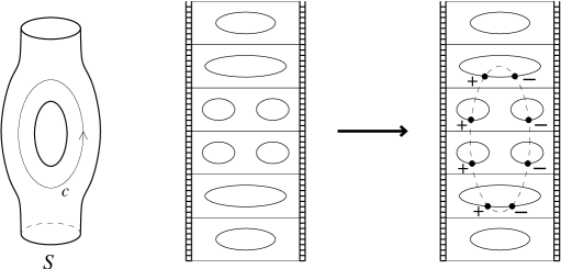
Figure 5.7: Inserting an oriented closed curve $c$ into a movie.

Hence we obtain an action of oriented closed curves on the set of framings of $S$. It is easy to see that this action coincides with the $H_{1}(S)$–action discussed in Section 5.2. Since the latter action is transitive, it follows that we can find a configuration of signed points whose insertion into $M^{\prime}$ changes $f^{\prime}$ into $f$.

2. Let $M^{\prime}$ and $M^{\prime\prime}$ be two signed movies representing isotopic framed cobordisms. Let $U(M^{\prime})$ and $U(M^{\prime\prime})$ denote the unsigned movies underlying $M^{\prime}$ and $M^{\prime\prime}$ (i.e. the movies $M^{\prime}$ and $M^{\prime\prime}$ without the signed points). By Theorem 1, there is a sequence of unsigned movies $M_{1},M_{2},\ldots,M_{m}$, such that $M_{1}=U(M^{\prime})$ and $M_{m}=U(M^{\prime\prime})$, and such that $M_{i}$ differs from $M_{i-1}$ by one of the Carter–Saito moves MM1–MM15.

By definition, the moves SM1–SM15 are signed analogues of the moves MM1–MM15. Hence we can lift the sequence $U(M^{\prime})=M_{1},M_{2},\ldots,M_{m}$ movie by movie to a sequence of signed movies $M^{\prime}=M^{\prime}_{1},M^{\prime}_{2},\ldots,M^{\prime}_{m}$, such that $U(M^{\prime}_{i})=M_{i}$ and such that $M^{\prime}_{i}$ differs from $M^{\prime}_{i-1}$ by one of the moves SM1–SM15, and possibly some of the additional moves SM16–SM20.

Let us explain the role of the additional moves. Assume we have already lifted the first $i-1$ movies $M_{1},M_{2},\ldots,M_{i-1}$ to a sequence $M^{\prime}_{1},M^{\prime}_{2},\ldots,M^{\prime}_{i-1}$. Since $M_{i}$ differs from $M_{i-1}$ by one of the moves MM1–MM15, it should be possible to insert signed points into $M_{i}$, so that the result is a signed movie $M^{\prime}_{i}$ differing from $M^{\prime}_{i-1}$ by one of the signed moves SM1–SM15. However, it might happen that the signed move is not directly applicable, for example because $M^{\prime}_{i-1}$ contains unwanted signed points, lying in the region of the cobordism where the signed move should take place. In this case, it is helpful to think of the unwanted points as oriented curves on the cobordism, as in the proof of part 1. By performing an isotopy, we can remove these curves from the relevant region of the cobordism. Back on the level of movies, this isotopy becomes a sequence of additional moves SM16–SM18. There are other cases, where moves SM19–SM20 are needed as well.

Now assume that we have lifted the entire sequence. Then it remains to show that $M^{\prime}_{m}$ and $M^{\prime\prime}$ are related by signed movie moves. Being lifts of the movie $M_{m}$, the movies $M^{\prime}_{m}$ and $M^{\prime\prime}$ agree, except possibly for the signed points. Moreover, since $M^{\prime}_{m}$ and $M^{\prime\prime}$ represent equivalent framings, the oriented curves $c^{\prime}_{m}$ and $c^{\prime\prime}$ coming from signed points in $M^{\prime}_{m}$ and in $M^{\prime\prime}$ must be homologous. To complete the proof, verify that any two homologous curves on a link cobordism can be related by a sequence of local modifications, which become the moves SM16–SM20 when seen on the level of movie presentations. $\Box$

Let FM1–FM20 denote the framed movie moves, obtained by replacing the signed points in SM1–SM20 by curls. Note that FM19 and FM20 are identical with FM1 and FM2.

Corollary 6

1. Every framed link cobordism has a framed movie presentation. 2. Two framed movies present isotopic framed link cobordisms if and only if there is a sequence of framed movie moves FM1–FM18 which takes one movie to the other.

Chapter 6 The colored Khovanov bracket

The colored Jones polynomial is the Reshetikhin–Turaev invariant [RT] for oriented framed links whose components are colored by irreducible representations of $U_{q}(\mathfrak{sl}(2))$. If all components are colored by the fundamental representation $V_{1}$, the colored Jones polynomial specializes to the ordinary Jones polynomial. The colored Jones polynomial plays an important role in the definition of the $\mathfrak{sl}(2)$ quantum invariant for $3$–manifolds and is conjecturally related to the hyperbolic volume of the knot complement.

Khovanov [Kh3] proposed two homology theories which have the colored Jones polynomial as the Euler characteristic.

In this chapter, we focus on Khovanov’s first theory, for the non–reduced colored Jones polynomial. We introduce a generalization of Khovanov’s theory, which we call the colored Khovanov bracket. We show that this theory is well–defined over $\mathbb{Z}$. Further, we introduce modifications of the colored Khovanov bracket, and study conditions under which colored framed link cobordisms induce chain transformations between our modified colored Khovanov brackets.

6.1 Colored Jones polynomial

Let $\mathbf{n}=(n_{1},\ldots,n_{l})$ be a finite sequence of non–negative integers. Let $(L,\mathbf{n})$ denote an oriented framed $l$–component link $L$ whose $n_{i}$–th component is colored by the $(n_{i}+1)$–dimensional irreducible representation $V_{n_{i}}$ of quantum $\mathfrak{sl}(2)$. Given a sequence $\mathbf{m}=(m_{1},\ldots,m_{l})$ of non–negative integers, we denote by $L^{\mathbf{m}}$ the $\mathbf{m}$–cable of $L$. When forming the $m_{i}$–cable of a component, we orient the strands by alternating the original and the opposite direction (starting with the original direction), so that neighbored strands are always oppositely oriented. The colored Jones polynomial $J(L,\mathbf{n})$ of the link $L$ can be expressed in terms of the Jones polynomial of its cables:

$$J(L,\mathbf{n})=\sum^{\lfloor{\mathbf{n}}/2\rfloor}_{{\mathbf{k}}=\mathbf{0}}(-1)^{|\mathbf{k}|}\left(\begin{array}[]{c}\mathbf{n}-\mathbf{k}\\ \mathbf{k}\end{array}\right)J(L^{\mathbf{n}-2\mathbf{k}})$$ (6.1)

where $|\mathbf{k}|=\sum_{i}k_{i}$ and

$$\left(\begin{array}[]{c}\mathbf{n}-\mathbf{k}\\ \mathbf{k}\end{array}\right)=\prod^{l}_{i=1}\left(\begin{array}[]{c}n_{i}-k_{i}\\ k_{i}\end{array}\right)\,.$$

In (6.1) the sum ranges over all $\mathbf{k}=(k_{1},\ldots,k_{l})$ such that $0\leq k_{i}\leq\lfloor n_{i}/2\rfloor$ for all $i$. Formula (6.1) is a consequence of the following relation, which holds in the representation ring of $U_{q}(\mathfrak{sl}(2))$ (for generic $q$), and which can be proved inductively using $V_{n}\otimes V_{1}\cong V_{n+1}\oplus V_{n-1}$:

$$V_{n}=\sum^{\lfloor n/2\rfloor}_{k=0}(-1)^{k}\left(\begin{array}[]{c}n-k\\ k\end{array}\right)V_{1}^{\otimes(n-2k)}\;.$$

Note that for $\mathbf{n}=(1,\ldots,1)$, we have $J(L,\mathbf{n})=J(L)$.

6.1.1 Graph $\Gamma_{\mathbf{n}}$.

The binomial coefficient $\left(\begin{array}[]{c}n-k\\ k\end{array}\right)$ equals the number of ways to select $k$ pairs of neighbors from $n$ dots placed on a vertical line, such that each dot appears in at most one pair. Analogously, $\left(\begin{array}[]{c}\mathbf{n}-\mathbf{k}\\ \mathbf{k}\end{array}\right)$ is the number of ways to select $\mathbf{k}$ pairs of neighbors on $l$ lines. We call such a selection of $\mathbf{k}$ pairs a $\mathbf{k}$–pairing. Given a $\mathbf{k}$–pairing $\mathbf{s}$, we denote by $D^{\mathbf{s}}$ the cable diagram containing only components corresponding to unpaired dots. Hence $D^{\mathbf{s}}$ is isotopic to $D^{\mathbf{n}-2\mathbf{k}}$.

Figure 6.1: The graph $\Gamma_{4,3}$.

Let $\Gamma_{\mathbf{n}}$ be the graph, whose vertices correspond to $\mathbf{k}$–pairings. Two vertices of $\Gamma_{\mathbf{n}}$ are connected by an edge if the corresponding pairings can be related to each other by adding/removing one pair of neighboring points. The “degree” of a vertex labeled by a $\mathbf{k}$–pairing is equal $|\mathbf{k}|$. The edges are directed towards increasing of degrees (see Figure 6.1).

6.2 Colored Khovanov bracket

Let $D$ be a diagram of an oriented framed link $L$ (framed by the blackboard framing) and let $\mathbf{n}=(n_{1},\ldots,n_{l})$ be a coloring of the components of $L$ by non–negative integers. To $(D,\mathbf{n})$ we associate a complex $\operatorname{Kh}(D,\mathbf{n})$ in the category $\operatorname{Mat}(\operatorname{gKob}_{/h})$. The construction goes as follows:

At each vertex of the graph $\Gamma_{\mathbf{n}}$ labeled by a $\mathbf{k}$–pairing $\mathbf{s}$ we put the complex $\operatorname{Kh}(D^{\mathbf{s}})$ defined as in (1.10), but viewed as an object of the homotopy category $\operatorname{gKob}_{/h}$. With an edge $e$ of $\Gamma_{\mathbf{n}}$ connecting a $\mathbf{k}$–pairing $\mathbf{s}$ to a $\mathbf{k}^{\prime}$–pairing $\mathbf{s}^{\prime}$, we associate a morphism $A_{e}:\operatorname{Kh}(D^{\mathbf{s}})\rightarrow\operatorname{Kh}(D^{\mathbf{s}^{\prime}})$ in the category $\operatorname{gKob}_{/h}$, as follows. Let $C$ and $C^{\prime}$ denote the two neighbored strands of the cable $L^{\mathbf{s}}$ which form a pair in $\mathbf{s}^{\prime}$ but not in $\mathbf{s}$. Consider a standard annulus glued between $C$ and $C^{\prime}$ (i.e. such that $C$ and $C^{\prime}$ are its boundary components, see [Kh3]). Assume that $L^{\mathbf{s}}$ is embedded in $\mathbb{R}^{3}\times[0,1]$ as $L^{\mathbf{s}}\times\{0\}$, and that the interior of the annulus is pushed into the interior of $\mathbb{R}^{3}\times[0,1]$. Let $S_{e}$ denote the link cobordism from $L^{\mathbf{s}}$ to $L^{\mathbf{s}^{\prime}}$ which is given by the annulus on $C$ and $C^{\prime}$ and by the identity cobordism on all other strands of $L^{\mathbf{s}}$. By Section 1.4, $S_{e}$ induces a morphism $\operatorname{Kh}(S_{e}):\operatorname{Kh}(D^{\mathbf{s}})\rightarrow\operatorname{Kh}(D^{\mathbf{s}^{\prime}})$ in $\operatorname{Kob}_{/h}$, which is well–defined up to sign. Define $A_{e}:=\operatorname{Kh}(S_{e})$ to be this morphism. Note that $A_{e}$ is graded of Jones degree zero because the Euler characteristic of an annulus is zero.

The sign of $A_{e}$ depends on the choice of the movie presentation for the annulus, but for any choice of movie presentations, the squares of $\Gamma_{\mathbf{n}}$ commute up to sign, because cobordisms given by gluing of annuli in a different order are isotopic. We call a choice of signs for the morphisms $A_{e}$ satisfactory if all squares anticommute.

Given a satisfactory choice of signs, we define a chain complex $\operatorname{Kh}(D,\mathbf{n})$ in the category $\operatorname{Mat}(\operatorname{gKob}_{/h})$ as follows. The $k$–th “chain space” is given by

$$\operatorname{Kh}(D,\mathbf{n})^{k}:=\bigoplus\operatorname{Kh}(D^{\mathbf{s}})\;\in\operatorname{Ob}(\operatorname{Mat}(\operatorname{gKob}_{/h}))$$

where the sum ranges over all $\mathbf{k}$–pairings $\mathbf{s}$ with $|\mathbf{k}|=k$. The $k$–th differential $d_{\mathbf{n}}^{k}:\operatorname{Kh}(D,\mathbf{n})^{k}\rightarrow\operatorname{Kh}(D,\mathbf{n})^{k+1}$ is given by $(d^{k}_{\mathbf{n}})_{\mathbf{s}^{\prime},\mathbf{s}}:=A_{e}$ whenever $\mathbf{s}$ and $\mathbf{s}^{\prime}$ are connected by an edge $e$, and $(d^{k}_{\mathbf{n}})_{\mathbf{s}^{\prime},\mathbf{s}}:=0$ otherwise (here $\mathbf{s}$ denotes a $\mathbf{k}$–pairing with $|\mathbf{k}|=k$, and $\mathbf{s}^{\prime}$ denotes a $\mathbf{k}^{\prime}$–pairing with $|\mathbf{k}^{\prime}|=k+1$). Since all squares of $\Gamma_{\mathbf{n}}$ anticommute, we get $d_{\mathbf{n}}^{k+1}\circ d_{\mathbf{n}}^{k}=0$.

Lemma 15

There exists a satisfactory choice of signs making all squares of $\Gamma_{\mathbf{n}}$ anticommute.

For the proof of Lemma 15, we need the following auxiliary observation. Claim. Let $e_{1},e_{2},\ldots,e_{m}$ be a sequence of oriented edges in $\Gamma_{\mathbf{n}}$, such that the starting point $e_{i+1}$ agrees with the endpoint of $e_{i}$. Then the composition $A:=A_{e_{m}}\circ\ldots\circ A_{e_{2}}\circ A_{e_{1}}$ is non–zero in $\operatorname{gKob}_{/h}$. More generally, $N$ times $A$ is non–zero for any integer $N\in\mathbb{Z}$, $N\neq 0$. In particular, $A$ is not equal to its negative. Proof of the claim. We only prove the first statement (i.e. that $A\neq 0$), but the more general statement follows in exactly the same way.

Let us start with the case where $D$ is the diagram of a knot colored by $n=2$. In this case, $\Gamma_{\mathbf{n}}$ has a single edge $e$, and we have to show that $A_{e}\neq 0$. Recall that $A_{e}$ is given by an embedded annulus in $\mathbb{R}^{3}\times[0,1]$. Let $\bar{A}_{e}$ denote the chain transformation obtained by turning $A_{e}$ upside–down (i.e. by reflecting $A_{e}$ along $\mathbb{R}^{3}\times\{1/2\}\subset\mathbb{R}^{3}\times[0,1]$). Then $\bar{A}_{e}\circ A_{e}:\operatorname{Kh}(\emptyset)\rightarrow\operatorname{Kh}(\emptyset)$ is induced by an embedded torus, which is isotopic in $\mathbb{R}^{4}$ to a trivially embedded torus. Using the (T) relation, we get $\bar{A}_{e}\circ A_{e}=\pm 2\operatorname{Id}$, where $\operatorname{Id}$ denotes the identity morphism of $\operatorname{Kh}(\emptyset)$, and hence $A_{e}\neq 0$ .

Similarly, if $D$ is a diagram of a knot colored by $n>2$, we can pre- and postcompose $A_{e_{m}}\circ\ldots\circ A_{e_{2}}\circ A_{e_{1}}$ with suitable cobordisms, in such a way that the result is either isotopic to a trivially embedded torus in $\mathbb{R}^{4}$ or to the identity cobordism of the knot. In both cases we get $A_{e_{m}}\circ\ldots\circ A_{e_{2}}\circ A_{e_{1}}\neq 0$.

Finally, if $D$ represents a link with more than one component, we can apply the above argument to the different components of the link individually. If necessary, we can use the (N) relation to unlink the resulting embedded tori from identity cobordisms. Details are left to the reader. $\Box$

Proof of Lemma 15. Let us first show that we can make all squares commute. We define a $1$–cochain $\zeta\in C^{1}(\Gamma_{\mathbf{n}},\mathbb{Z}/2\mathbb{Z})$ as follows. For any square $S\subset\Gamma_{\mathbf{n}}$, we put $\zeta(S)=0$ if $S$ is commutative, and $\zeta(S)=1$ if $S$ is anticommmutative. Note that $\zeta$ is well–defined because of the above claim. Using that $\mathbb{Z}/2\mathbb{Z}$ is a field, we can extend $\zeta$ to a $1$–cochain. Now it is easy to see that all squares of $\Gamma_{\mathbf{n}}$ become commutative if we replace $A_{e}$ by $(-1)^{\zeta(e)}A_{e}$.

Once all squares commute, we can make them anticommute as follows. For each edge $e$, connecting two pairings $\mathbf{s}$ and $\mathbf{s}^{\prime}$, we multiply the morphism $A_{e}$ by $(-1)^{(\mathbf{s},\mathbf{s}^{\prime})}$, where $(\mathbf{s},\mathbf{s}^{\prime})$ denotes the number of pairs in $\mathbf{s}$, which lie either on the same vertical line as unique pair in $\mathbf{s}^{\prime}\backslash\mathbf{s}$ and above that pair, or on one of the vertical lines to the right of that pair (see Figure 6.1). $\Box$

Lemma 16

Different satisfactory choices of signs lead to isomorphic complexes. Moreover, for any two satisfactory choices of signs there is a preferred isomorphism between the corresponding complexes.

Proof. Consider two choices of signs, given by two $1$–cochains $\zeta$ and $\zeta^{\prime}$ as in the proof of Lemma 15. If both choices of signs are satisfactory, we must have $\zeta(S)=\zeta^{\prime}(S)$ for all squares $S\subset\Gamma_{\mathbf{n}}$. Since the space $Z_{1}(\Gamma_{\mathbf{n}},\mathbb{Z}/2\mathbb{Z})$ of $1$–cycles of $\Gamma_{\mathbf{n}}$ is generated by squares, $\zeta$ and $\zeta^{\prime}$ must coincide on $Z_{1}(\Gamma_{\mathbf{n}},\mathbb{Z}/2\mathbb{Z})$, and therefore $\zeta-\zeta^{\prime}=\delta\gamma$ for a $0$–chain $\gamma\in C^{0}(\Gamma_{\mathbf{n}},\mathbb{Z}/2\mathbb{Z})$. Now note that for every edge $e$ of $\Gamma_{\mathbf{n}}$ with boundary $s-s^{\prime}$, we have $\zeta(e)-\zeta^{\prime}(e)=\gamma(s)-\gamma(s^{\prime})$. Therefore, the morphisms $(-1)^{\gamma(s)}\operatorname{Id}_{\operatorname{Kh}(D^{s})}$ define an isomorphism between the complex associated to $\zeta$ and the complex associated to $\zeta^{\prime}$.

To see that there is a preferred choice for the isomorphism between the $\zeta$– and the $\zeta^{\prime}$–complex, observe that any two $0$–cochains $\gamma$ as above must differ by a $0$–cocycle. Since the space of $0$–cocycles of $\Gamma_{\mathbf{n}}$ is isomorphic to $\mathbb{Z}/2\mathbb{Z}$, there are only two possible choices for $\gamma$. The preferred $\gamma$ is the one which maps the left–most vertex of $\Gamma_{\mathbf{n}}$ to $0$. $\Box$ Alternatively, Lemma 16 can be proved by constructing the preferred isomorphism explicitly, by defining it to be the identity on the left–most vertex of $\Gamma_{\mathbf{n}}$ and then extending it arrow by arrow to the right.

Lemmas 15 and 16 show that $\operatorname{Kh}(D,\mathbf{n})$ is well–defined up to canonical isomorphism. We call $\operatorname{Kh}(D,\mathbf{n})$ the colored Khovanov bracket of $(D,\mathbf{n})$.

Remark. By definition, the colored Khovanov bracket is an element of $\operatorname{Kom}(\operatorname{Mat}(\operatorname{Kom}_{/h}(\text{{g}}{\mathcal{C}ob}_{\bullet/l}^{3})))$, and hence a “complex of complexes”. However it is not a bicomplex, because the $A_{e}$ are just homotopy classes of chain transformations (rather than honest chain transformations). We do not know whether it is possible to lift $\operatorname{Kh}(D,\mathbf{n})$ to a bicomplex by choosing suitable representatives for the homotopy classes $A_{e}$.

Theorem 14

The isomorphism class of $\operatorname{Kh}(D,\mathbf{n})$ is an invariant of the colored oriented framed link $(L,\mathbf{n})$.

Proof. If $(D,\mathbf{n})$ and $(D^{\prime},\mathbf{n})$ represent isotopic colored framed links $(L,\mathbf{n})$ and $(L^{\prime},\mathbf{n})$, then the cables $L^{\mathbf{s}}$ and $L^{\prime\mathbf{s}}$ are isotopic as well. In particular, the complexes $\operatorname{Kh}(D^{\mathbf{s}})$ and $\operatorname{Kh}(D^{\prime\mathbf{s}})$ are isomorphic as objects of $\operatorname{gKob}_{/h}$. This shows that $\operatorname{Kh}(D,\mathbf{n})$ and $\operatorname{Kh}(D^{\prime},\mathbf{n})$ are isomorphic on the level of objects. The isotopy between $L^{\mathbf{s}}$ and ${L^{\prime}}^{\mathbf{s}}$ extends to an isotopy between the annuli appearing in the definition of the differentials. Hence Theorem 3 and Lemma 16 imply that $\operatorname{Kh}(D,\mathbf{n})$ and $\operatorname{Kh}(D^{\prime},\mathbf{n})$ are isomorphic as complexes. $\Box$

Let $\mathcal{C}(D,\mathbf{n}):=\mathcal{F}_{\operatorname{Kh}}(\operatorname{Kh}(D,\mathbf{n}))$ and $\mathcal{C}^{\prime}(D,\mathbf{n}):=\mathcal{F}_{\operatorname{Lee}}(\operatorname{Kh}(D,\mathbf{n}))$. The total graded Euler characteristic of $\mathcal{C}(D,\mathbf{n})$ is defined by

$$\tilde{\chi}_{q}(\mathcal{C}(D,\mathbf{n})):=\sum_{k,i,j}(-1)^{k+i}q^{j}\dim_{\mathbb{Q}}(\mathcal{C}^{k,i,j}(D,\mathbf{n})\otimes\mathbb{Q})$$

where $k$,$i$ and $j$ respectively refer to the homological grading of $\mathcal{C}(D,\mathbf{n})$, the homological grading of the complexes $\mathcal{C}(D^{\mathbf{n}-2\mathbf{k}})$, and the Jones grading of the complexes $\mathcal{C}(D^{\mathbf{n}-2\mathbf{k}})$.

Theorem 15

The total graded Euler characteristic of $\mathcal{C}(D,\mathbf{n})$ is equal to the colored Jones polynomial $J(L,\mathbf{n})$.

Proof. We have

$$\begin{split}\tilde{\chi}_{q}(\mathcal{C}(D,\mathbf{n}))&=\sum_{k,i,j}(-1)^{k+i}q^{j}\dim_{\mathbb{Q}}(\mathcal{C}^{k,i,j}(D,\mathbf{n})\otimes\mathbb{Q})\\ &=\sum_{k}(-1)^{k}\sum_{|\mathbf{k}|=k}\sum_{\mathbf{s}\in{I_{\mathbf{k}}}}\chi_{q}(\mathcal{C}(D^{\mathbf{n}-2\mathbf{k}}))\\ &=\sum^{\lfloor\mathbf{n}/2\rfloor}_{\mathbf{k}=\bf 0}(-1)^{|\mathbf{k}|}\left(\begin{array}[]{c}\mathbf{n}-\mathbf{k}\\ \mathbf{k}\end{array}\right)\chi_{q}(\mathcal{C}(D^{\mathbf{n}-2\mathbf{k}}))\end{split}$$

where in the second line $I_{\mathbf{k}}$ denotes the set of all $\mathbf{k}$–pairings. Taking into account that $\chi_{q}(\mathcal{C}(D^{\mathbf{n}-2\mathbf{k}}))=J(L^{\mathbf{n}-2\mathbf{k}})$ and comparing with (6.1) we get the result. $\Box$

6.3 Modified colored Khovanov bracket

In the following, we assume that the additional relation $\raisebox{-5.69046pt}{\psfig{height=17.07182pt}}=0$ is imposed on the category ${\mathcal{C}ob}_{\bullet/l}^{3}$.

6.3.1 Modified differentials.

Let us generalize the definition of $\operatorname{Kh}(D,\mathbf{n})$ as follows. As before, we put $\operatorname{Kh}(D^{\mathbf{n}-2\mathbf{k}})$ at vertices of $\Gamma_{\mathbf{n}}$ labeled by $\mathbf{k}$–pairings. But we modify the morphisms associated to edges of $\Gamma_{\mathbf{n}}$. With an edge $e$ connecting $\mathbf{k}$– and $\mathbf{k}^{\prime}$–pairings we associate the morphism

$$A^{\prime}_{e}:=\alpha A_{e}+\beta A^{\bullet}_{e}\;,$$

where $\alpha,\beta\in\mathbb{Z}$ are fixed integers integers and where $A^{\bullet}_{e}:=A_{e}\circ X_{e}$. The morphism $X_{e}$ will be defined below. Note that the sign of $A_{e}$ depends on the choice of a movie presentation for the annulus, but the relative sign between $A_{e}$ and $A^{\bullet}_{e}$ is independent of any choice. Given a satisfactory choice of signs, the result is a chain complex which we denote $\operatorname{Kh}(D,\mathbf{n})_{\alpha,\beta}$. Observe that $\operatorname{Kh}(D,\mathbf{n})_{1,0}=\operatorname{Kh}(D,\mathbf{n})$. The morphism $X_{e}$ is graded of Jones degree $-2$. Hence if $\beta$ is non–zero, then the morphisms $A^{\prime}_{e}$ do not respect the Jones degree anymore.

6.3.2 The morphism $X_{e}$.

$X_{e}$ is defined as follows. Let $C_{i}$ and $C_{i+1}$ be the two strands of the cable $D^{\mathbf{n}-2\mathbf{k}}$ which are annihilated by $A_{e}$, i.e. which do not appear in $D^{\mathbf{n}-2\mathbf{k}^{\prime}}$ anymore. For a point $P$ on $C_{i}$, let $X_{P}$ denote the endomorphism of $\operatorname{Kh}(D^{\mathbf{n}-2\mathbf{k}})$ induced “multiplying” with a dot at the point $P$ (i.e. $X_{P}$ is induced by the identity cobordism of $D^{\mathbf{n}-2\mathbf{k}}$, decorated by a single dot, located near the point $P$). According to Lemma 5 (Section 1.4), $X_{P}$ changes its sign when $P$ slides across a crossing. To fix the sign, we checkerboard color the regions of $D^{\mathbf{n}-2\mathbf{k}}$, such that the unbounded region is colored white, and we define $\sigma(P):=+1$ or $\sigma(P):=-1$, depending on whether the region between $C_{i}$ and $C_{i+1}$, which lies next to $P$, is black or white. Now the product $\sigma(P)X_{P}$ is independent of the choice of $P$. We define $X_{e}:=\sigma(P)X_{P}$. If $C_{i}$ and $C_{i+1}$ belong to the cable of a component $K$ of the link represented by $D$, we will also use the notation $X(K,i)$ for $X_{e}$.

6.4 Towards functoriality

Let ${\mathcal{C}ob}_{f}^{4}$ be the category of colored framed movie presentations. The objects are diagrams of colored links and the morphisms movie presentations of colored framed links, i.e. sequences of colored link diagrams, where between two consecutive diagrams one of the following transformations occurs: FR1, R2 or R3, or a saddle, a cap or a cup. Note that here we need to distinguish between two saddle moves: a “splitting” saddle which splits one colored component into two of the same color, and a “merging” saddle which merges two components of the same color into one component.

We are interested in a construction of a functor

$$\operatorname{Kh}_{\alpha,\beta}:{\mathcal{C}ob}_{f}^{4}\rightarrow\operatorname{Kom}(\operatorname{Mat}(\operatorname{Kob}_{/h}))\;.$$

Given two colored link diagrams $(D,\mathbf{n})$ and $(D_{0},\mathbf{n}_{0})$ which are related by a Reidemeister move, a cap, a cup or a saddle, we would like to associate a chain transformation

$$F:\operatorname{Kh}_{\alpha,\beta}(D,\mathbf{n})\longrightarrow\operatorname{Kh}_{\alpha,\beta}(D_{0},\mathbf{n}_{0})\;.$$

We can do this by specifiying “matrix elements”

$$F_{\mathbf{s}_{0},\mathbf{s}}:\operatorname{Kh}_{\alpha,\beta}(D^{\mathbf{s}})\longrightarrow\operatorname{Kh}_{\alpha,\beta}(D_{0}^{\mathbf{s}_{0}})\;$$

for all pairings $\mathbf{s}$ of $\mathbf{n}$ and all pairings $\mathbf{s}_{0}$ of $\mathbf{n}_{0}$. For Reidemeister moves, we can take the matrix elements implicit in the proof of Theorem 14. Subsections 6.4.1, 6.4.2 and 6.4.3 are devoted to the definition of matrix elements corresponding to cap, cup and saddles.

Throughout this section, we assume the additional relation $\raisebox{-5.69046pt}{\psfig{height=17.07182pt}}=0$. Moreover, we assume that $2$ is made invertible, i.e. that the morphism sets of ${\mathcal{C}ob}_{\bullet/l}^{3}$ are tensored by $\mathbb{Z}[1/2]$.

6.4.1 Cup and cap.

Let $(D,\mathbf{n})$ and $(D_{0},\mathbf{n}_{0})$ be two colored link diagrams which are related by a cup cobordism. Assume that $D_{0}$ is the disjoint union of $D$ with a trivial component $K=\bigcirc$, and that $\mathbf{n}_{0}$ restricts to $\mathbf{n}$ on $D$ and to an arbitrary color $n$ on $K$. Given a pairing $\mathbf{s}$ of $\mathbf{n}$ and a pairing $\mathbf{s}_{0}$ of $\mathbf{n}_{0}$, we define a morphism

$$\iota_{\mathbf{s}_{0},\mathbf{s}}:\operatorname{Kh}(D^{\mathbf{s}})\longrightarrow\operatorname{Kh}(D_{0}^{\mathbf{s}_{0}})$$

as follows: $\iota_{\mathbf{s}_{0},\mathbf{s}}$ is non–zero only if the restriction of $\mathbf{s}_{0}$ to $K$ is the empty pairing (no pairs) and if $\mathbf{s}_{0}$ agrees with $\mathbf{s}$ on all other components. In this case, we put $\iota_{\mathbf{s},\mathbf{s}_{0}}:=G\circ C$, where $C:\operatorname{Kh}(D^{\mathbf{s}})\rightarrow\operatorname{Kh}(D^{\mathbf{s}_{0}})$ is the morphism induced by a union of $n$ cups whose boundaries are the $n$ strands of the $n$–cable of $K$, and $G$ is the endomorphism of $\operatorname{Kh}(D^{\mathbf{s}_{0}})$ defined by

$$G:=\sum_{j=1}^{n}Y_{j}\circ Z_{j}\;.$$

Here, $Y_{j}$ is the composition of all morphisms $(\alpha\operatorname{Id}-\beta X(K,i))/2$ for $1\leq i\leq j$, and $Z_{j}$ is the composition of all morphisms $(\alpha\operatorname{Id}+\beta X(K,i))/2$ for $j<i\leq n$. $\alpha$ and $\beta$ are the same integers as in the definition of the modified differentials.

Now let $(D,\mathbf{n})$ and $(D_{0},\mathbf{n}_{0})$ be two colored link diagrams related by a cap cobordism. Assume that $D$ is the disjoint union of $D_{0}$ with a trivial component $K$, and that $\mathbf{n}$ restricts to $\mathbf{n}_{0}$ on $D_{0}$ and to an arbitrary color $n$ on $K$. We define

$$\epsilon_{\mathbf{s}_{0},\mathbf{s}}:\operatorname{Kh}(D^{\mathbf{s}})\longrightarrow\operatorname{Kh}(D_{0}^{\mathbf{s}_{0}})$$

as follows: $\epsilon_{\mathbf{s}_{0},\mathbf{s}}$ is non–zero only if the restriction of $\mathbf{s}$ to $K$ is the empty pairing and if $\mathbf{s}$ agrees with $\mathbf{s}_{0}$ on all other components. In this case, we define $\epsilon_{\mathbf{s}_{0},\mathbf{s}}:=\bar{C}\circ G$ where $G$ is the endomorphism of $\operatorname{Kh}(D^{\mathbf{s}})$ defined as above, and $\bar{C}$ is the morphism induced by $n$ caps whose boundaries are the $n$ strands of the $n$–cable of $K$.

6.4.2 Merging saddle.

Let $(D,\mathbf{n})$ and $(D_{0},\mathbf{n}_{0})$ be two colored link diagrams which are related by a saddle merging two components $K_{1}$ and $K_{2}$ of $D$ into a single component $K$ of $D_{0}$. Assume that $\mathbf{n}$ and $\mathbf{n}_{0}$ restrict to a color $n$ on the components $K_{1}$, $K_{2}$ and $K$, and that they are identical on all other components.

Let $\mathbf{s}$ be a pairing of the $\mathbf{n}$–cable of $D$, and let $s_{1}$ and $s_{2}$ denote its restrictions to $K_{1}$ and $K_{2}$, respectively. Let $s_{1}\cup s_{2}$ denote the union of $s_{1}$ and $s_{2}$, i.e. the pairing of $n$ which consists of all pairs which are contained in either $s_{1}$ or in $s_{2}$ or in both. Given $\gamma,\delta\in\mathbb{Z}$ and a pairing $\mathbf{s}_{0}$ of the $\mathbf{n}_{0}$–cable of $D_{0}$, we define a morphism

$$m^{\gamma,\delta}_{\mathbf{s}_{0},\mathbf{s}}:\operatorname{Kh}(D^{\mathbf{s}})\longrightarrow\operatorname{Kh}(D^{\mathbf{s}_{0}})$$

as follows. $m^{\gamma,\delta}_{\mathbf{s}_{0},\mathbf{s}}$ is zero unless the following is satisfied:

• $s_{1}$ and $s_{2}$ have no common dot (meaning that there is no dot which belongs to a pair both in $s_{1}$ and in $s_{2}$),

• $\mathbf{s}_{0}$ is the pairing which restricts to $s_{1}\cup s_{2}$ on $K$ and which agrees with $\mathbf{s}$ on all other components.

If the above conditions are satisfied, we put $m^{\gamma,\delta}_{\mathbf{s}_{0},\mathbf{s}}:=F_{3}\circ F_{2}\circ F_{1},$ where $F_{1},F_{2}$ and $F_{3}$ are defined as follows.

• $F_{1}$ is the endomorphism of $\operatorname{Kh}(D^{\mathbf{s}})$ defined by $F_{1}:=X_{1}\circ X_{2}$, where $X_{1}$ is the composition of all $(\gamma\operatorname{Id}+\delta X(K_{1},i))/2$ such that the dots numbered $i$ and $i+1$ form a pair in $s_{2}$, and $X_{2}$ is the composition of all $(\gamma\operatorname{Id}+\delta X(K_{2},i))/2$ such that the dots numbered $i$ and $i+1$ form a pair in $s_{1}$.

• Let $\mathbf{s}^{\prime}$ be the pairing of $\mathbf{n}$ which restricts to $s_{1}\cup s_{2}$ on both $K_{1}$ and $K_{2}$ and which agrees with the pairing $\mathbf{s}$ on all other components of $D$. $F_{2}:\operatorname{Kh}(D^{\mathbf{s}})\rightarrow\operatorname{Kh}(D^{\mathbf{s}^{\prime}})$ is the morphism induced by attaching annuli to the strands of $K_{1}^{s_{1}}$ and $K_{2}^{s_{2}}$ according to the following rule. If the two dots numbered $i$ and $i+1$ form a pair in $s_{2}$, we attach an annulus to the strands numbered $i$ and $i+1$ in $K_{1}^{s_{1}}$. Similarly, if the two dots numbered $i$ and $i+1$ form a pair in $s_{1}$, we attach an annulus to the strands numbered $i$ and $i+1$ in $K_{2}^{s_{2}}$.

• $F_{3}:\operatorname{Kh}(D^{\mathbf{s}^{\prime}})\rightarrow\operatorname{Kh}(D^{\mathbf{s}_{0}})$ is the morphism obtained by merging each strand of $K_{1}^{s_{1}\cup s_{2}}$ with the corresponding strand of $K_{2}^{s_{1}\cup s_{2}}$ by a saddle cobordism.

The above construction mimics a construction of Khovanov [Kh3]. Khovanov’s map $\psi$ corresponds to our morphism $m^{0,2}_{\mathbf{s}_{0},\mathbf{s}}$. Note that $m^{0,\delta}_{\mathbf{s}_{0},\mathbf{s}}$ is graded of Jones degree $\deg(m^{0,\delta}_{\mathbf{s}_{0},\mathbf{s}})=-n$, where $n$ is the color of the components $K_{1}$,$K_{2}$ and $K$. We denote by $m^{\gamma,\delta}$ the collection of all morphisms $m^{\gamma,\delta}_{\mathbf{s}_{0},\mathbf{s}}$.

6.4.3 Splitting saddle.

Suppose the diagrams $(D,\mathbf{n})$ and $(D_{0},\mathbf{n}_{0})$ are related by a saddle which splits a component $K$ of $D$ into two components $K_{1}$ and $K_{2}$ of $D_{0}$. Assume that the colorings $\mathbf{n}$ and $\mathbf{n}_{0}$ are consistent with each other, in the obvious sense. Consider a pairing $\mathbf{s}$ of the $\mathbf{n}$–cable of $D$ which restricts to a $k$–pairing $s$ on $K$. Given $\gamma,\delta\in\mathbb{Z}$ and a pairing $\mathbf{s}_{0}$ of the $\mathbf{n}_{0}$–cable of $D_{0}$, we define a morphism

$$\Delta^{\gamma,\delta}_{\mathbf{s}_{0},\mathbf{s}}:\operatorname{Kh}(D^{\mathbf{s}})\longrightarrow\operatorname{Kh}(D_{0}^{\mathbf{s}_{0}})$$

as follows. $\Delta^{\gamma,\delta}_{\mathbf{s}_{0},\mathbf{s}}$ is zero unless $\mathbf{s}_{0}$ has the following properties:

• the restrictions $s_{1}$ and $s_{2}$ of $\mathbf{s}_{0}$ to $K_{1}$ and $K_{2}$ have no common dot,

• the union of $s_{1}$ and $s_{2}$ is equal to $s$,

• $\mathbf{s}_{0}$ agrees with $\mathbf{s}$ on all components of $D_{0}$ other than $K_{1}$ and $K_{2}$.

If $\mathbf{s}_{0}$ satisfies the above properties, we define $\Delta^{\gamma,\delta}_{\mathbf{s}_{0},\mathbf{s}}:=2^{k}\bar{F}_{1}\circ\bar{F}_{2}\circ\bar{F}_{3}$, where $\bar{F}_{1},\bar{F}_{2}$ and $\bar{F}_{3}$ are the morphisms obtained by turning the morphisms $F_{1},F_{2}$ and $F_{3}$ of Subsection 6.4.2 upside down (i.e. by reflecting the link cobordisms appearing in the definition of $F_{1},F_{2}$ and $F_{3}$ along the hyperplane $\mathbb{R}^{3}\times\{1/2\}$).

6.4.4 Criteria for chain transformations.

In this subsection, we give criteria under which the matrix elements $m^{\gamma,\delta}_{\mathbf{s}_{0},\mathbf{s}}$ and $\Delta^{\gamma,\delta}_{\mathbf{s}_{0},\mathbf{s}}$ induce chain transformations. To simplify the notation, we will drop the superscripts $\gamma,\delta$ in $m^{\gamma,\delta}$ and $\Delta^{\gamma,\delta}$ and just write $m$ and $\Delta$.

Let us first consider the case of merging saddles. Let $(D,\mathbf{n})$ and $(D_{0},\mathbf{n}_{0})$ be two colored link diagrams which are related by a merging saddle, and let $d$ and $d_{0}$ denote the differentials of $\operatorname{Kh}(D,\mathbf{n})_{\alpha,\beta}$ and $\operatorname{Kh}(D_{0},\mathbf{n}_{0})_{\alpha,\beta}$, respectively. Let $\mathbf{s}$ be a pairing of $\mathbf{n}$, and let $\mathbf{s}_{0}$ be the pairing of $\mathbf{n}_{0}$ which restricts to $s_{1}\cup s_{2}$ on $K$ and which agrees with $\mathbf{s}$ on all other components (here, $s_{1}$, $s_{2}$ and $K$ are defined as in Subsection 6.4.3). For a pairing $\mathbf{s}_{0}^{\prime}$ of $\mathbf{n}_{0}$, we wish to compare the matrix elements $(d_{0}\circ m)_{\mathbf{s}_{0}^{\prime},\mathbf{s}}$ and $(m\circ d)_{\mathbf{s}_{0}^{\prime},\mathbf{s}}$. Assume that at least one of these matrix elements is non–zero. This is only possible if $s_{1}$ and $s_{2}$ have no common dot. Moreover, $\mathbf{s}_{0}^{\prime}$ must contain a unique pair $p$ which does not appear in $\mathbf{s}_{0}$, and otherwise be identical with $\mathbf{s}_{0}$. We assume that $p$ lies on $K$ (for otherwise $(d_{0}\circ m)_{\mathbf{s}_{0}^{\prime},\mathbf{s}}=\pm(m\circ d_{0})_{\mathbf{s}_{0}^{\prime},\mathbf{s}}$ is trivially satisfied). Then we are in the situation of (6.2), where we have left away all dots corresponding to strands on which $(d_{0}\circ m)_{\mathbf{s}_{0}^{\prime},\mathbf{s}}$ and $(m\circ d_{0})_{\mathbf{s}_{0}^{\prime},\mathbf{s}}$ agree trivially, and where $d^{\prime}:=d_{\mathbf{s}^{\prime},\mathbf{s}}$, $d^{\prime\prime}:=d_{\mathbf{s}^{\prime\prime},\mathbf{s}}$ and $d_{0}^{\prime}:=(d_{0})_{\mathbf{s}_{0}^{\prime},\mathbf{s}_{0}}$. Note that $p$ is the pair in the upper right corner.

(6.2)

Lemma 17

Assume that $d^{\prime}_{0}\circ m_{\mathbf{s}_{0},\mathbf{s}}=\pm(m_{\mathbf{s}_{0}^{\prime},\mathbf{s}^{\prime}}\circ d^{\prime}+m_{\mathbf{s}_{0}^{\prime},\mathbf{s}^{\prime\prime}}\circ d^{\prime\prime})$ for all diagrams as in (6.2). Then there is a $0$–cochain $\gamma\in C^{0}(\Gamma_{\mathbf{n}},\mathbb{Z}/2\mathbb{Z})$ such that the morphisms $F_{\mathbf{s}_{0},\mathbf{s}}:=(-1)^{\gamma(\mathbf{s})}m_{\mathbf{s}_{0},\mathbf{s}}$ determine a chain transformation between $\operatorname{Kh}(D,\mathbf{n})_{\alpha,\beta}$ and $\operatorname{Kh}(D_{0},\mathbf{n}_{0})_{\alpha,\beta}$, i.e. such that $d_{0}\circ F=F\circ d$.

The proof of Lemma 17 is quite technical, so we skip it here and instead refer to [BW].

Now assume that $(D,\mathbf{n})$ and $(D_{0},\mathbf{n}_{0})$ are related by a splitting saddle. Let $\mathbf{s}$ be a pairing of the $\mathbf{n}$–cable of $D$ and let $\mathbf{s}_{0}^{\prime}$ be a pairing of the $\mathbf{n}_{0}$–cable of $D_{0}$, such that at least one of the morphisms $(d_{0}\circ\Delta)_{\mathbf{s}_{0}^{\prime},\mathbf{s}}$ and $(\Delta\circ d)_{\mathbf{s}_{0}^{\prime},\mathbf{s}}$ is non–zero. Let $K$ denote the component of $D$ which is involved in the saddle and let $s$ be the restriction of $\mathbf{s}$ to $K$. Similarly, let $K_{1}$ and $K_{2}$ be the components of $D_{0}$ which are involved in the saddle and let $s_{1}^{\prime}$ and $s_{2}^{\prime}$ denote the restrictions of $\mathbf{s}_{0}^{\prime}$ to $K_{1}$ and $K_{2}$. Then every pair of $s$ must also appear in the union $s_{1}^{\prime}\cup s_{2}^{\prime}$. If $s_{1}^{\prime}$ and $s_{2}^{\prime}$ have a common pair, we are in the situation of (6.3).

(6.3)

Now assume that $s_{1}^{\prime}$ and $s_{2}^{\prime}$ have no common pair. Let $s_{1}$ and $s_{2}$ denote the intersections $s_{1}:=s\cap s_{1}^{\prime}$ and $s_{2}:=s\cap s_{2}^{\prime}$. Let $\mathbf{s}_{0}$ denote the pairing of the $\mathbf{n}_{0}$–cable of $D_{0}$ which restricts to $s_{1}$ and $s_{2}$ on the components $K_{1}$ and $K_{2}$ and which agrees with $\mathbf{s}$ on all other components of $D_{0}$. Then every pair of $\mathbf{s}_{0}$ must also be a pair of $\mathbf{s}_{0}^{\prime}$. Moreover, $\mathbf{s}_{0}^{\prime}$ has to contain a unique pair $p$ which is not contained in $\mathbf{s}_{0}$. We assume that $p$ belongs to $K_{1}$ or $K_{2}$ (for otherwise $(d_{0}\circ\Delta)_{\mathbf{s}_{0}^{\prime},\mathbf{s}}=\pm(\Delta\circ d)_{\mathbf{s}_{0}^{\prime},\mathbf{s}}$ is trivially satisfied). If $p$ is disjoint from all pairs of $s_{1}\cup s_{2}$, we are in the situation of (6.4), where $p$ is the pair in the upper right corner.

(6.4)

It is also possible that $p$ has a common dot with a pair of $s_{1}\cup s_{2}$. Examples of this case are shown in (6.5).

(6.5)

Lemma 18

Assume that the squares of (6.4) commute, up to sign, and assume that $d_{0}\circ\Delta_{\mathbf{s}_{0},\mathbf{s}}=0$ for all squares as in (6.5). Then there is a $0$–cochain $\gamma\in C^{0}(\Gamma_{\mathbf{n}_{0}},\mathbb{Z}/2\mathbb{Z})$ such that the morphisms $(-1)^{\gamma(\mathbf{s}_{0})}\Delta_{\mathbf{s}_{0},\mathbf{s}}$ determine a chain transformation between $\operatorname{Kh}(D,\mathbf{n})_{\alpha,\beta}$ and $\operatorname{Kh}(D_{0},\mathbf{n}_{0})_{\alpha,\beta}$.

In Lemma 18, no assumption has to be made about the diagrams of (6.3). Indeed, if the squares of (6.4) commute, then the anticommutativity of the squares of $\Gamma_{\mathbf{n}_{0}}$ implies $d_{0}^{\prime}\circ\Delta^{\prime}+d_{0}^{\prime\prime}\circ\Delta^{\prime}=0$ for all diagrams as in (6.3).

6.4.5 Chain transformations.

Theorem 16

For $\alpha=\beta=1$, the maps $\mathcal{F}_{\rm Lee}(m_{\mathbf{s}_{0},\mathbf{s}}^{1,1})$ and $\mathcal{F}_{\rm Lee}(\Delta_{\mathbf{s}_{0},\mathbf{s}}^{1,1})$ induce chain transformations.

Sketch of the proof. We have to show that for $\alpha=\beta=1$, the morphisms $\mathcal{F}_{\operatorname{Lee}}(m_{\mathbf{s}_{0},\mathbf{s}}^{1,1})$ and $\mathcal{F}_{\operatorname{Lee}}(\Delta_{\mathbf{s}_{0},\mathbf{s}}^{1,1})$ satisfy the conditions of Lemmas 17 and 18.

We start with the proof of $\mathcal{F}_{\operatorname{Lee}}(d_{0}\circ\Delta^{1,1}_{\mathbf{s}_{0},\mathbf{s}})=0$ for the left square of (6.5). Assume that the three dots in the lower left corner of the square are numbered from bottom to top from $i$ to $i+2$. Moreover, assume that these dots lie on a component $K$ of $D$, and that the saddle cobordism splits $K$ into components $K_{1}$ and $K_{2}$. (In the left square of (6.5), $K_{1}$ and $K_{2}$ correspond to the left and the right column of dots in the upper left corner). Let $s_{2}$ denote the restriction of $\mathbf{s}_{0}$ to $K_{2}$, and let $C_{i}$, $C_{i+1}$ and $C_{i+2}$ denote the strands of $K_{2}^{s_{2}}$ corresponding to the dots $i$, $i+1$ and $i+2$, respectively. For $\alpha=\beta=1$, $d_{0}$ is given by

$$A_{i+1}\circ(\operatorname{Id}+X(K_{2},i+1))$$

where $A_{i+1}$ is induced by an annulus attached to the components $C_{i+1}$ and $C_{i+2}$ of $K_{2}^{s_{2}}$. Similarly, $\Delta^{1,1}_{\mathbf{s}_{0},\mathbf{s}}$ is given by some saddle cobordisms, composed with

$$(\operatorname{Id}+X(K_{2},i))\circ\bar{A}_{i}$$

where $\bar{A}_{i}$ is induced by an annulus attached to $C_{i}$ and $C_{i+1}$. We can replace $X(K_{2},i)$ by $-X(K_{2},i+1)$ because we can move the point $P$ used in the definition of $X(K_{2},i)=\sigma(P)X_{P}$ across the annulus. The minus sign appears because of the definition of $\sigma(P)$. Summarizing, we see that $d_{0}\circ\Delta^{1,1}_{\mathbf{s}_{0},\mathbf{s}}$ factors through

$$(\operatorname{Id}+X(K_{2},i+1)))\circ(\operatorname{Id}-X(K_{2},i+1))=\operatorname{Id}-X(K_{2},i+1)^{2}\,.$$

Now recall that in Lee’s Frobenius algebra, we have the relation $X^{2}={\bf 1}$. Hence $\mathcal{F}_{\operatorname{Lee}}(\operatorname{Id}-X(K_{2},i+1)^{2})=0$ and therefore $\mathcal{F}_{\operatorname{Lee}}(d_{0}\circ\Delta^{1,1}_{\mathbf{s}_{0},\mathbf{s}})=0$. So the left square of (6.5) commutes. The proof for the right square is analogous.

To show that the squares of (6.4) commute up to sign, one has to apply isotopies, the (N) relation and the defining relations for Lee’s functor to the cobordisms corresponding to $(d_{0}\circ\Delta^{1,1})_{\mathbf{s}_{0}^{\prime},\mathbf{s}}$, $(\Delta^{1,1}\circ d)_{\mathbf{s}_{0}^{\prime},\mathbf{s}}$. Similarly, to prove that the assumption of Lemma 17 is satisfied, on has to apply the same relations to $(d_{0}\circ m^{1,1})_{\mathbf{s}_{0}^{\prime},\mathbf{s}}$, and $(m^{1,1}\circ d)_{\mathbf{s}_{0}^{\prime},\mathbf{s}}$. $\Box$

Theorem 17

For $\alpha=\beta=1$, the maps $\mathcal{F}_{\operatorname{Lee}}(\epsilon_{\mathbf{s}_{0},\mathbf{s}})$ and $\mathcal{F}_{\operatorname{Lee}}(\iota_{\mathbf{s}_{0},\mathbf{s}})$ associated to caps and cups induce chain transformations.

Proof. The case of caps is easy, so we only discuss the case of cups. Let $D$ and $D_{0}$ be two link diagrams which are related by a cup cobordism, i.e. $D_{0}=D\sqcup K$ for a trivial component $K$.

Let $d$ and $d_{0}$ denote the differentials of $\operatorname{Kh}(D,\mathbf{n})_{\alpha,\beta}$ and $\operatorname{Kh}(D_{0},\mathbf{n}_{0})_{\alpha,\beta}$, respectively. We write $d_{0}$ as $d_{0}=d_{0}^{\prime}+d_{0}^{\prime\prime}$, where $d_{0}^{\prime}$ denotes the sum of all $A^{\prime}_{e}$ which contract a pair on $K$, and $d_{0}^{\prime\prime}$ denotes the sum of all $A^{\prime}_{e}$ which contract a pair on one of the other components of $D_{0}$. Then $d_{0}^{\prime\prime}\circ\iota=\iota\circ d$, so we must show that $\mathcal{F}_{\operatorname{Lee}}(d_{0}^{\prime}\circ\iota)=0$.

For $\alpha=\beta=1$, $d_{0}^{\prime}$ is a sum of morphisms

$$A^{\prime}_{i}=A_{i}\circ(\operatorname{Id}+X(K,i))=A_{i}\circ(\operatorname{Id}-X(K,i+1))\,,$$

where $A_{i}$ is induced by an annulus glued to the strands $i$ and $i+1$ of the cable of $K$. $\iota$ is equal to $G\circ C$, where $G=\sum_{j=0}^{n}Y_{j}\circ Z_{j}$. Using $X^{2}={\bf 1}$ and the definitions of $Y_{j}$ and $Z_{j}$ with $\alpha=\beta=1$, we get

$$\mathcal{F}_{\rm Lee}((\operatorname{Id}+X(K,i))\circ Y_{j})=0$$

for $i\leq j$, and

$$\mathcal{F}_{\rm Lee}((\operatorname{Id}-X(K,i+1))\circ Z_{j})=0$$

for $i\geq j$. Hence $\mathcal{F}_{\rm Lee}(A^{\prime}_{i}\circ Y_{j}\circ Z_{j})=0$ for all $i,j$, and therefore $\mathcal{F}_{\rm Lee}(d_{0}^{\prime}\circ\iota)=0$. $\Box$

Assume we can make the definition of the chain transformations in Theorems 16 and 17 canonical, i.e. independent of any sign choices. Then $\mathcal{F}_{\operatorname{Lee}}(\operatorname{Kh}_{1,1}(D,\mathbf{n}))$ extends to a well–defined functor $\mathcal{F}_{\operatorname{Lee}}\circ\operatorname{Kh}_{1,1}:{\mathcal{C}ob}^{4}_{f}\rightarrow\operatorname{Kom}(\operatorname{Kom}_{/h}(\mathbb{Z}\mbox{-}\operatorname{mod}))$. Let ${\mathcal{C}ob}_{f/i}^{4}$ denote the quotient of ${\mathcal{C}ob}_{f}^{4}$ by framed movie moves. We expect Conjecture. The functor $\mathcal{F}_{\operatorname{Lee}}\circ\operatorname{Kh}_{1,1}$ descends to a functor $\mathcal{F}_{\operatorname{Lee}}\circ\operatorname{Kh}_{1,1}:{\mathcal{C}ob}_{f/i}^{4}\rightarrow\operatorname{Kom}_{/\pm h}(\operatorname{Kom}_{/h}(\mathbb{Z}\mbox{-}\operatorname{mod}))$.

In [BW], we also defined chain transformations for $\mathcal{F}_{\operatorname{Kh}}(\operatorname{Kh}(D,\mathbf{n})_{0,1})$:

Theorem 18

For $\alpha=0$, $\beta=1$, the maps $\mathcal{F}_{\operatorname{Kh}}(m_{\mathbf{s}_{0},\mathbf{s}}^{0,1})$, $\mathcal{F}_{\operatorname{Kh}}(\Delta_{\mathbf{s}_{0},\mathbf{s}}^{0,1})$, $\mathcal{F}_{\operatorname{Kh}}(\epsilon_{\mathbf{s}_{0},\mathbf{s}})$ and $\mathcal{F}_{\operatorname{Kh}}(\iota_{\mathbf{s}_{0},\mathbf{s}})$ induce chain transformations.

The proof of Theorem 18 is analogous to the proofs of Theorems 16 and 17.

Remark. We do not know how to extend the original colored Khovanov bracket $\operatorname{Kh}(D,\mathbf{n})=\operatorname{Kh}(D,\mathbf{n})_{1,0}$ to a functor. For the original colored Khovanov bracket, the morphisms $m_{\mathbf{s}_{0},\mathbf{s}}^{0,2}$ induce chain transformations (cf. [Kh3]), but there is no choice of $\gamma,\delta$ for which the $\Delta_{\mathbf{s}_{0},\mathbf{s}}^{\gamma,\delta}$ induce chain transformations.

Bibliography

- [AP] M. Asaeda and J. Przytycki, Khovanov homology: torsion and thickness, arXiv:math.GT/0402402.
- [B1] D. Bar–Natan, On Khovanov’s Categorification of the Jones polynomial, Algebraic and Geometric Topology 2 (2002) 337–370, arXiv:math.QA/0201043.
- [B2] D. Bar–Natan, Khovanov’s homology for tangles and cobordisms, Geometry & Topology, vol. 9 (2005) 1443–1499, arXiv: math.GT/0410495.
- [B3] D. Bar–Natan, Fast Khovanov homology computations, arXiv: math.GT/0606318.
- [B4] D. Bar–Natan, Mutation Invariance of Khovanov Homology, http://katlas.math.toronto.edu/drorbn/index.php?title=Mutation_ Invariance_of_Khovanov_Homology
- [BM] D. Bar–Natan, S. Morrison, The Karoubi envelope and Lee’s degeneration of Khovanov homology, arXiv:math.GT/0606542.
- [BW] A. Beliakova, S. Wehrli, Categorification of the colored Jones polynomial and Rasmussen invariant of links, to appear in the Canadian Math. J., arXiv:math.QA/0510382.
- [CF] D. Cimasoni, V. Florens, Generalized Seifert surfaces and signature of colored links, to appear in Trans. AMS, arXiv:math.GT/0505185.
- [CK] A. Champanerkar, I. Kofman, Spanning trees and Khovanov homology, arXiv:math.GT/0607510.
- [Co] John H. Conway, An enumeration of knots and links and some of their related properties, Computational problems in Abstract Algebra, Pergamon Press, New York, 329-358, 1970.
- [CS] S. Carter, M. Saito, Reidemeister moves for surface isotopies and their interpretation as moves to movies, J. Knot Theory Ramific. 2 (1993) 251–284
- [Ja] M. Jacobsson, An invariant of link cobordisms from Khovanov homology, Algebr. Geom. Topol. 4 (2004) 1211–1251.
- [Jo] V. Jones, A polynomial invariant for knots via von Neumann algebras, Bull. Amer. Math. Soc., vol.12 (1985) no. 1, 103–111.
- [Ka1] L. H. Kauffman, Formal Knot Theory, Mathematical Notes 30, Princeton University Press (1983).
- [Ka2] L. H. Kauffman, State models and the Jones polynomial, Topology 26 (1987) 395–407.
- [Kaw] A. Kawauchi, A Survey of Knot Theory, Birkhäuser 1996.
- [Kh1] M. Khovanov, A categorification of the Jones polynomial, Duke Math. J. 101 (2000) no. 3, 359–426, arXiv:math.QA/9908171.
- [Kh2] M. Khovanov, An invariant of tangle cobordisms, Trans. Amer. Math. Soc. 358 (2006) 315–327, arXiv:math.QA/0207264.
- [Kh3] M. Khovanov, Categorifications of the colored Jones polynomial, J. Knot Theory Ramific. 14 (2005) 111–130, arXiv:math.QA/0302060.
- [Kh4] M. Khovanov, Link homology and Frobenius extensions, Fund. Math., 190 (2006) 179–190, arXiv: math.QA/0411447.
- [KR1] M. Khovanov, L. Rozansky, Matrix factorizations and link homology, arXiv:math.QA/0401268.
- [KR2] M. Khovanov, L. Rozansky, Matrix factorizations and link homology II, arXiv:math.QA/0505056.
- [L1] E. S. Lee, The support of Khovanov’s invariants for alternating knots, arXiv:math.GT/0201105.
- [L2] E. S. Lee, On Khovanov invariant for alternating links, arXiv: math.GT/0210213.
- [Mu] J. Murakami, The Parallel Version of Polynomial Invariants of Links, Osaka J. Math. 26 (1989) 1–55.
- [OS1] P. Ozsváth and Z. Szabó, Knot Floer homology, genus bounds, and mutation, arXiv:math.GT/0303225.
- [OS2] P. Ozsváth and Z. Szabó On the Heegaard Floer homology of branched double–covers, Adv. Math. 194 (2005) no. 1, 1–38, arXiv: math.GT/0309170.
- [Ra] J. Rasmussen, Khovanov homology and the slice genus, arXiv: math.GT/0402131.
- [RT] N. Reshetikhin, V. Turaev, Invariants of –manifolds via link polynomials and quantum groups, Invent. Math. 103 (1991) 547–598.
- [S1] A. Shumakovitch, KhoHo, Basel 2002, see http://www. geometrie.ch/KhoHo.
- [S2] A. Shumakovitch, Rasmussen invariant, slice–Bennequin inequality, and sliceness of knots, arXiv:math.GT/0411643.
- [T] M. B. Thistlethwaite, A spanning tree expansion of the Jones polynomial, Topology 26 (1987) 297–309.
- [V] O. Viro, Remarks on the definition of Khovanov Homology, arXiv:math.GT/0202199.
- [We1] S. Wehrli, Khovanov Homology and Conway Mutation, arXiv: math.GT/0301312.
- [We2] S. Wehrli, A spanning tree model for Khovanov homology, arXiv: math.GT/0409328.
- [Wu] H. Wu, Legendrian Links and the Spanning Tree Model for Khovanov Homology, arXiv:math.GT/0605630.