The role of optimization on the human dynamics of tasks execution

Abstract

In order to explain the empirical evidence that the dynamics of human activity may not be well modeled by Poisson processes, a model based on queuing processes were built in the literature [bar05]. The main assumption behind that model is that people execute their tasks based on a protocol that execute firstly the high priority item. In this context, the purpose of this letter is to analyze the validity of that hypothesis assuming that people are rational agents that make their decisions in order minimize the cost of keeping non-executed tasks on the list. Therefore, we build and solve analytically a dynamic programming model with two priority types of tasks and show that the validity of this hypothesis depends strongly on the structure of the instantaneous costs that a person has to face if a given task is kept on the list for more than one step. Moreover, one interesting finding is that in one of the situations the protocol used to execute the tasks generates complex one dimensional dynamics.

Department of Economics, Catholic University of Brasilia, 70790-160, Brasilia, DF, Brazil.

1 Introduction

Empirical evidence has shown that the dynamics of inter-event times driven by human actions may not be random and not well approximated by Poisson processes [paxflo96, masmon03, sca06]. Based on this, Barabási [bar05] developed a very interesting model of human activity where the distribution of the inter-event time is a consequence of a decision queue processes. He considers that among the most relevant protocols for driving human dynamics, e.g. first-in-first-out protocol, random protocol and a protocol based on the execution of the high priority item, this later protocol seems to be the most important. In this protocol, while high priority tasks are executed as soon as they are added to the list, low priority tasks wait for a long time until all high priority tasks are executed, i.e., the instants of execution of low priority tasks are separated by long times of inactivity. Using this assumption, it is numerically [bar05] (analytically [vaz05]) shown that the distribution of inter-event times follows a power law.

Two interesting contributions were introduced by [grilin06]. First the authors map the variable length priority model considered above onto a model of biased diffusion deriving asymptotic distributions for the inter-event times. Second, in order to investigate the arising of power laws in more general situations, they generalize the fixed length model queue to contain tasks with a priority label and with a class label where there is always an active class and an inactive class. If the highest priority task of the inactive class exceeds that of the active class by at least a fixed switching cost, the inactive class becomes active and the active class becomes inactive.

An interesting discussion is considered in [ken06, baroli06] where it is argued that other mechanisms contribute for the distributions of waiting times such as deadlines, time dependence of priorities and the social context of the problem. In line with this debate, [bla06] relaxes the assumption that the priorities of tasks do not change over time and studies queueing systems where deadlines are assigned to the incoming tasks and the urgency to attend a task increases with time showing that only in the former model fat tails arise naturally as consequence of the scheduling rule.

In this letter, we investigate the assumption that people execute tasks on a protocol that execute firstly the high priority item. In particular, we suppose that people assign priorities to the tasks on their lists in order to minimize some cost index, i.e., a cost associated to the fact of not processing a given collection of tasks in a given time step. Therefore, based on this assumption and inspired on [bar05, vaz05, grilin06], we have built a discounted stochastic dynamic programming model with two types of tasks (low and high priority tasks) and a cost per stage for keeping a number of low and high priority tasks without processing.

This is not the first time that a kind of optimization principle is used to understand the structure and dynamics of complex systems. In [rodrin92, caj05], for instance, it is shown that complex networks may arise from optimization principles.

It is also important to stress that although there is a large literature dealing with control of queue discipline [cra77, kitryk95, sen99] which this work is related, the model presented in this letter is neither an extension nor a particular case of any of these results.

We have found that the type of protocol used to execute tasks is strongly dependent on the kind of instantaneous cost of keeping a task in the queue for an additional stage. When linear costs are used the protocol of executing preferentially the high priority costs always is the best solution. However, this does not happen when quadratic costs are considered. In this case different types of protocol are considered. Furthermore, depending on the parameters of the system, the protocol considered generates complex one dimensional dynamics.

2 Setup of the problem

We consider that there are two queues waiting for a service on a single server. Let $g(x_{L},x_{H})$ be the current cost of having state $(x_{L},x_{H})$ which is the state of the system, $x_{L}$ ($x_{H}$) is the number of tasks in the first (second) queue. We say that the first queue is a low priority queue (or the second queue is a high priority queue) if $\frac{\partial g(x_{L},x_{H})}{\partial x_{L}}|_{x_{L}=x_{H}}<\frac{\partial g(x_{L},x_{H})}{\partial x_{H}}|_{x_{L}=x_{H}}$. We assume that this is the case. The dynamics of these queues are modeled as follows: At each discrete time step with probability $\lambda\rho$ a new task arrives in the queue formed by high priority tasks and with probability $\lambda(1-\rho)$ a new task arrives in the queue formed by low priority tasks. Within each of the queues the tasks are executed on a First-In, First-Out basis. With probability $\mu u(x_{L},x_{H})$ the first task of the high priority queue is executed and with probability $\mu(1-u(x_{L},x_{H}))$ the first task of the low priority queue is executed. We assume here that $u(x_{L},x_{H})$ is a state dependent control variable that the agent will choose in order to minimize the total cost function $J_{u}(x_{L},x_{H})=E_{x_{L},x_{H}}^{u}[\sum_{t=1}^{\infty}\alpha^{t}g((x_{L}(t),x_{H}(t)))]$, where $E_{x_{L},x_{H}}^{u}[\cdot]$ is the expected value conditioned to the current state $(x_{L},x_{H})$ and the state control variable $u$ and $\alpha$ is the discount factor.

Due to the principle of optimality [bel57, ber01] and the Banach fixed point theorem, if the minimum cost function $J(x_{L},x_{H})=\min_{u(x_{L},x_{H})\in[0,1]}J_{u}(x_{L},x_{H})$ exists, it must be given by the unique solution of the Bellman equation, that may be written as

$$J(x_{L},x_{H})=F(x_{L},x_{H})+\min_{u(x_{L},x_{H})\in[0,1]}u(x_{L},x_{H})G(x_{L},x_{H})$$ (1)

where

$$F(x_{L},x_{H}) = g(x_{L},x_{H})+\lambda\rho(1-\mu)[\alpha J(x_{L},x_{H}+1)]$$ (2)

$$+ \lambda(1-\rho)(1-\mu)[\alpha J(x_{L}+1,x_{H})]$$

$$+ (1-\lambda)\mu[\alpha J(x_{L}-1,x_{H})]$$

$$+ \rho\lambda\mu[\alpha J(x_{L}-1,x_{H}+1)]$$

$$+ (1-\rho)\lambda\mu[\alpha J(x_{L},x_{H})]$$

$$+ (1-\lambda)(1-\mu)[\alpha J(x_{L},x_{H})]$$

and

$$G(x_{L},x_{H})=$$ (3)

$$(1-\lambda)\mu[\alpha(J(x_{L},x_{H}-1)-J(x_{L}-1,x_{H}))]$$

$$+ \rho\lambda\mu[\alpha(J(x_{L},x_{H})-J(x_{L}-1,x_{H}+1))]$$

$$+ (1-\rho)\lambda\mu[\alpha(J(x_{L}+1,x_{H}-1)-J(x_{L},x_{H}))]$$

Since the optimization problem (1) is a linear programming problem, the optimal control $u(x_{L},x_{H})$ in each state $(x_{L},x_{H})$ will depend explicitly on the signal of $G(x_{L},x_{H})$. If $G(x_{L},x_{H})>0$, then $u(x_{L},x_{H})=0$. If $G(x_{L},x_{H})<0$, then $u(x_{L},x_{H})=1$. Finally, if $G(x_{L},x_{H})=0$, $u(x_{L},x_{H})$ is a mixed strategy that may present any value in the interval $[0,1]$. It is quite intuitive this result. Indeed, one may note that the terms in square brackets defined in $G(x_{L},x_{H})$, equation (3), comprises the variations in the cost function due to changes in the states of the queue related to the execution of one of the tasks.

Since the properties of the solution of $J(x_{L},x_{H})$ of the Bellman equation (1) are strongly dependent on choice of the cost per stage $g(x_{L},x_{H})$, in the next sections, two different choices for $g(x_{L},x_{H})$ are investigated.

3 Linear costs

In this section, we assume that $g(x_{L},x_{H})=h_{L}x_{L}+h_{H}x_{H}$, for $0<h_{L}<h_{H}$, i.e., the current cost of having one additional high priority task in the queue is larger than having one additional low priority task in the queue.

Since the space of polynomials of degree 1 with sup-norm is a Banach space, one can show inductively, making recursive iterations of the dynamic programming mapping, that $J(x_{L},x_{H})$ is also linear. Therefore, for $x_{L}>0$ and $x_{H}>0$, guessing this form, one may easily solve the Bellman equation (1) and show that the cost function is given by

$$J(x_{L},x_{H})=c+c_{L}x_{L}+c_{H}x_{H}$$ (4)

Furthermore,

$$G(x_{L},x_{H})=\mu\frac{\alpha}{1-\alpha}(h_{L}-h_{H})$$ (5)

is always negative implying that $u(x_{L},x_{H})=u=1$ for every state $(x_{L},x_{H})$. Therefore, if linear costs are considered, the protocol to be considered is the one based on the execution of the high priority task whenever there is at least one item in this queue, i.e., $x_{H}>0$. This kind of protocol was very well studied in [bar05, vaz05, grilin06] where analytic results for the emerging of power laws may be found. In the next section, a much wealthier situation happens where the optimal policy is not only limited to execute the high priority item in the queue, but the optimal policy is state-dependent.

4 Quadratic costs

Now, we assume that $g(x_{L},x_{H})=h_{L}x_{L}^{2}+h_{H}x_{H}^{2}$, for $0<h_{L}<h_{H}$. Following the same reasoning already presented before for the linear cost case, one may conclude a quadratic form for the cost function.

Solving the Bellman equation, one may show that the solution of the problem depends explicitly on the signal of the function $G(x_{L},x_{H})$, defined in (3), in the state $(x_{L},x_{H})$. In fact, three different regions will arise. We will call region $A$ the domain of $(x_{L},x_{H})$ where $G(x_{L},x_{H})>0$, region $B$ the domain of $(x_{L},x_{H})$ where $G(x_{L},x_{H})=0$ and region $C$ the domain of $(x_{L},x_{H})$ where $G(x_{L},x_{H})<0$.

We have found that the minimum cost function is given by

$$J(x_{L},x_{H})=\left\{\begin{array}[]{c}J^{A}(x_{L},x_{H})\;\mathrm{if}\;(x_{L},x_{H})\in A\\ J^{B}(x_{L},x_{H})\;\mathrm{if}\;(x_{L},x_{H})\in B\\ J^{C}(x_{L},x_{H})\;\mathrm{if}\;(x_{L},x_{H})\in C\\ \end{array}\right.$$ (6)

and the optimal control is given by

$$u(x_{L},x_{H})=\left\{\begin{array}[]{c}0\;\mathrm{if}\;(x_{L},x_{H})\in A\\ u\in[0,1]\;\mathrm{if}\;(x_{L},x_{H})\in B\\ 1\;\mathrm{if}\;(x_{L},x_{H})\in C\\ \end{array}\right.$$ (7)

where for $i=A,B,C$

$$J^{i}(x_{L},x_{H}) = c^{i}+c_{L1}^{i}x_{L}+c_{H1}^{i}x_{H}+c_{L2}x_{L}^{2}+c_{H2}x_{H}^{2}$$

$$G^{i}(x_{L},x_{H}) = \mu[c_{L1}^{i}-c_{H1}^{i}+2(c_{L2}x_{l}-c_{H2}x_{H})$$

$$+ c_{L2}(2\lambda(1-\rho)-1)+c_{H2}(1-2\lambda\rho)]$$

and $G(x_{L},x_{H})=G^{i}(x_{L},x_{H})$, if $(x_{L},x_{H})\in i$ .

Furthermore, the parameter $\delta\in[\underline{\delta},\overline{\delta}]$, defines the set of points of $\Re^{2}$ such that $G(x_{L},(h_{L}/h_{H})x_{L}+\delta)=0$ .

Indeed,

$$\delta\rightarrow\underline{\delta}\Rightarrow\left(J^{B}(\delta)\rightarrow J^{A},\;G^{B}(\delta)\rightarrow G^{A}\right)$$ (10)

and

$$\delta\rightarrow\overline{\delta}\Rightarrow\left(J^{B}(\delta)\rightarrow J^{C},\;G^{B}(\delta)\rightarrow G^{C}\right)$$ (11)

In order to understand the intuition behind this solution, one is invited to consider a particular case where $h_{L}/h_{H}\approx 1$, $\lambda=\mu=1$ and $\rho=1/2$. In this case, the region $B$ is defined by the set of points where $|x_{H}-x_{L}|<\alpha/(1-\alpha)$. Therefore, the set of points where the decision maker can use any strategy depends strictly on the discount factor. If the discount factor is large, the decision maker may keep queues with a large difference between their sizes. On the other hand, if the discount factor is small this situation is not accepted as a solution anymore.

Figure 1: The regions $A$, $B$ and $C$ in the plane $x_{L}-x_{H}$.

Differently from the linear costs case, several types of protocol are possible. Region $C$ considers a protocol based on the execution of the high priority task. Region $A$ considers a protocol based on the execution of the low priority task. It occurs in order to avoid that the size of the queue of the low priority tasks do not increase too much. “Too much” here is measured by the ratio $h_{L}/h_{H}$. Region $B$ does not determine a protocol. It can be a random protocol (mixed strategy) or simply a protocol such the one considered in region $C$ or region $A$. Figure 1 shows the geometry of these regions in the plane $x_{L}-x_{H}$.

It is not difficult to show that the expected value of the state obeys the following dynamics

$$E_{t}[x(t + 1)]=E_{t}\left[\begin{array}[]{c}x_{L}(t+1)\\ x_{H}(t+1)\\ \end{array}\right]=\left[\begin{array}[]{c}x_{L}(t)\\ x_{H}(t)\\ \end{array}\right]$$ (16)

$$+ \left[\begin{array}[]{c}\lambda(1-\rho)-\mu(1-u(x_{L}(t),x_{H}(t)))\\ \lambda\rho-\mu u(x_{L}(t),x_{H}(t))\\ \end{array}\right]$$ (19)

which has infinite fixed points if and only if $\lambda=\mu$ and $u(x_{L},x_{H})=u=\rho$.

We will analyze only the most interesting situation which is the fixed-length-queue, i.e., $\lambda=\mu$. Therefore, assuming that $\lambda=\mu$, $u^{B}=\rho+\epsilon$ and $\epsilon>0$, then the expected value of the system is governed by $E_{t}[x(t+1)]=x(t)+\lambda\epsilon e$ if it is in region $B$ and by $E_{t}[x(t+1)]=x(t)-\lambda\rho e$ if it is in region $A$ (if the state is in region $C$, the expected state will certainly come to region $B$ and not come back to this region), where $e=(1,-1)^{\prime}$. Therefore, the dynamics takes place in the line passing by $x(0)$ and following the direction $e$. Thus, if the expected state is in region $B$ it goes into the direction of region $A$ and viceversa. This dynamics is equivalent to the one dimensional system

$$y(t+1)=\left\{\begin{array}[]{c}y(t)+t^{+}\;\mathrm{if}\;y(t)\leq 0\\ y(t)-t^{-}\;\mathrm{if}\;y(t)>0\\ \end{array}\right.$$ (20)

defined on the interval $(-t^{-},t^{+}]$, where $t^{+}=\lambda\epsilon$ and $t^{-}=\lambda\rho$

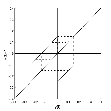
Figure 2: The evolution of $y(t)$ for $y_{0}=-0.2$, $\lambda=0.5$, $\rho=0.5$ and $\epsilon=0.3$.

The dynamics of this system is plotted in figure 2 for the case of $t^{-}=0.25$ and $t^{+}=0.15$. The dynamics defined in (20) is topologically conjugate with the translation in the circle [dem93]. Therefore, if $t^{+}/t^{-}=p/q$, where $p/q$ is a irreducible ratio representation of rational number, then this system follows a limit cycle with period $p+q$. Otherwise, the $\omega$-limit of any point in the interval is a dense subset of it. Therefore, we can conclude that the stochastic process that defines the length of each queue is not stationary. Moreover, the dynamics of the expected value of the length of the queue exhibits a complex behavior: infinitely many cycles or a $\omega$-limit set being a dense subset in the interval. The intuition behind that complex dynamics is quite reasonable. In the region close to the frontier $x_{H}=(h_{L}/h_{H})x_{L}+\underline{\delta}$ that separate $A$ and $B$ (see figure 1), we can observe the following: if the expected state is in $A$, its dynamics moves toward region B, since the priority is of $L$ . Once the expected state is in $B$, the dynamics takes it back to the region A, since in this case in average the priority is of $H$ (due to the condition $u^{B}=\rho+\epsilon$ and $\epsilon>0$). Because the frequency of tasks arriving is equal to that of attending them, a cyclical or complex dynamics emerges close to the referred frontier. Figure 2 shows the case where this system is a limit cycle. A similar situation involving regions $B$ and $C$ arises in the case of $\epsilon>0$ and $\rho=u^{B}+\epsilon$. In these situations, the protocol is ruled by the protocols considered in regions $A$ and $B$ in the former case and by the protocols considered in regions $B$ and $C$ in the later case.

For $\lambda\neq\mu$, either the expected value goes to infinite, converges to 0, to axis $x_{L}=0$ or to axis $x_{H}=0$, following different routes. Furthermore, different kinds of protocols are possible.

5 Final Remarks

In the human dynamics of the tasks execution decisions the priority of one task is not always defined as being the most important current task. Actually, the dynamics of the work executions depends on the cumulated tasks of short run priorities, the importance of each kind of task and the intertemporal discount factor. In this letter, we provide a stochastic dynamic programming model containing all those elements and analyze the dynamics of the execution of tasks, shedding new light to the discursion considered in [ken06, baroli06]. In this setting, we have found that the dynamics of the expected state of the system may be complex, exhibiting cycles of any order or with limit set being a dense subset of the interval depending on the parameter values of the model. This is a contribution to a better understanding of how human dynamics may evolve in this type of problem. Finally, it is worth noting that complex dynamics in the solution of dynamic programming problems are usually obtained for low discount factors [monsor96]. However, in our quadratic case, complex dynamics arises for discount factors of any size.

6 Acknowledgment

The authors are indebt to the Brazilian agency CNPQ for financial support. The first author is also indebt to Professor G. Grinstein (at IBM Watson Research Center) who helped him by means of a personal communication to understand some details of his paper [grilin06].

References

- [1] \harvarditemBarabasi2005bar05 Barabasi, A. L. \harvardyearleft2005\harvardyearright. The origin of bursts and heavy tails in human dynamics, Nature 435: 207–211.
- [2] \harvarditemBarabasi \harvardand Oliveira2006baroli06 Barabasi, A. L. \harvardand Oliveira, J. G. \harvardyearleft2006\harvardyearright. Correspondence paterns, Nature 441: 04902.
- [3] \harvarditemBellman1957bel57 Bellman, R. \harvardyearleft1957\harvardyearright. Dynamic programming, Princeton University Press, New Jersey.
- [4] \harvarditemBertsekas2001ber01 Bertsekas, D. P. \harvardyearleft2001\harvardyearright. Dynamic programming and optimal control, Vol. II, Athena Scientific, Belmont.
- [5] \harvarditemBlanchard \harvardand Hongler2007bla06 Blanchard, P. \harvardand Hongler, M. O. \harvardyearleft2007\harvardyearright. Modeling human activity in the spirit of barabasi’s queueing systems, Physical Review E 75: 026102.
- [6] \harvarditemCajueiro2005caj05 Cajueiro, D. O. \harvardyearleft2005\harvardyearright. Agent preferences and the topology of networks, Physical Review E 72: 047104.
- [7] \harvarditem[Crabill et al.]Crabill, Gross \harvardand Magazine1977cra77 Crabill, T. B., Gross, D. \harvardand Magazine, M. J. \harvardyearleft1977\harvardyearright. A classified bibliography of research on optimal design and control of queues, Operations Research 25: 219–232.
- [8] \harvarditemDeMello \harvardand VanStrien1993dem93 DeMello, W. \harvardand VanStrien, S. \harvardyearleft1993\harvardyearright. One dimensional dynamics, Springer.
- [9] \harvarditemGrinstein \harvardand Linsker2006grilin06 Grinstein, G. \harvardand Linsker, R. \harvardyearleft2006\harvardyearright. Biased diffusion and universality in model queues, Physical Review Letters 97: 130201.
- [10] \harvarditemKentsis2005ken06 Kentsis, A. \harvardyearleft2005\harvardyearright. Mechanisms and models of human dynamics, Nature 441: 04901.
- [11] \harvarditemKitaev \harvardand Rykov1995kitryk95 Kitaev, M. Y. \harvardand Rykov, V. V. \harvardyearleft1995\harvardyearright. Controlled queueing systems, CRC Press, Boca Raton.
- [12] \harvarditem[Masoliver et al.]Masoliver, Montero \harvardand Weiss2003masmon03 Masoliver, J., Montero, M. \harvardand Weiss, G. H. \harvardyearleft2003\harvardyearright. Continuous time random walk model for financial distributions., Physical Review E 67: 021112.
- [13] \harvarditemMontrucchio \harvardand Sorger1996monsor96 Montrucchio, L. \harvardand Sorger, G. \harvardyearleft1996\harvardyearright. Topological entropy of policy functions in concave dynamic optimization models, Journal of Mathematical Economics 25: 181–194.
- [14] \harvarditemPaxson \harvardand Floyd1996paxflo96 Paxson, V. \harvardand Floyd, S. \harvardyearleft1996\harvardyearright. Wide-area trafic: the failure of poisson modeling., IEEE/ACM Transactions on Networks 3: 226.
- [15] \harvarditem[Rodriguez-Iturbe et al.]Rodriguez-Iturbe, Rinaldo, Rigon, Bras, Ijjasz-Vasquez \harvardand Marani1992rodrin92 Rodriguez-Iturbe, I., Rinaldo, A., Rigon, R., Bras, R. L., Ijjasz-Vasquez, E. \harvardand Marani, A. \harvardyearleft1992\harvardyearright. Fractal structures as least energy patterns - the case of river networks, Geophysical Research Letters 19: 889–892.
- [16] \harvarditem[Scalas et al.]Scalas, Kaizoji, Kirchler, Huber \harvardand Tedeschi2006sca06 Scalas, E., Kaizoji, T., Kirchler, M., Huber, J. \harvardand Tedeschi, A. \harvardyearleft2006\harvardyearright. Waiting times between orders and trades in double action markets, Physica A 366: 463–471.
- [17] \harvarditemSennott1999sen99 Sennott, L. I. \harvardyearleft1999\harvardyearright. Stochastic dynamic programming and the control of queueing systems, John Wiley and Sons, New York.
- [18] \harvarditemVázquez2005vaz05 Vázquez, A. \harvardyearleft2005\harvardyearright. Exact results for the barabási model of human dynamics, Physical Review Letters 95: 248701.
- [19]