Equipectrality and Transplantation

Abstract.

We present a technique novel in numerical methods. It compiles the domain of the numerical methods as a discretized volume. Congruent elements are glued together to compile the domain over which the solution of a boundary value problem of a linear operator is sought. We associate a group and a graph to that volume. When the group is symmetry of the boundary value problem under investigation, one can specify the structure of the solution, and find out if there are equispectral volumes of a given type. We show that similarity of the so called auxiliary matrices is sufficient and necessary for two discretized volumes to be equispectral. A simple example demonstrates the feasibility of the suggested method.

1. Problem description

In both science and engineering, we solve boundary values in a volume composed of large number of meshes. This is the case in nuclear engineering [1], in fluid dynamics [2], [3] and electromagnetic fields [4]. We address the question: under what conditions are the solutions for two meshes identical, or, are the solutions transformable into each other by a simple rule? How to find the transformation rule? How can we find equivalent meshes?

In the design and safety analysis of large industrial devices, calculational models are tested against experiments carried out on a small scale mock-up. This is the case with nuclear power plants [5], aeroplanes [6], and ships [7]. We would need a transplantation of the measured values to the geometry of the real scale device. Is there any hope of doing that exactly or have we to put up with approximate methods [8]?

In the sequel, we assume operator $\mathbf{A}$ to be a linear operator defined in a finite domain $V$ in $\mathbb{R}^{2}$ and to commute with the symmetry group of the plane $\mathbb{R}^{2}$. As to its physical meaning, the authors had in their minds the Laplace operator occurring in several physical problems from electricity to quantum physics, the diffusion and/or transport operators as used in reactor physics with homogeneous material distributions. The boundary value problem considered in the sequel is of Cauchy type (solution is zero along the boundary of $V$), but the authors are convinced that generalization to Neumann or third type boundary value problem is straightforward.

We suggest using discretized volumes. The domain $V$, over which the solution of the boundary value problem is sought is constructed by the following procedure. We choose an appropriate simply connected tile $t$, which in our cases is an $n$-gon and glue copies of the tile by their corresponding sides. Although in principle $t$ is almost arbitrary [9], we confine the discourse to triangular shaped tiles. Since triangulation is a well known and widely used technique even in theoretical problems [10], this is not considered as a limitation. The discretized volumes considered by us are always finite. A concise description of the structure of a discretized volume $V$ is a finitely presented group G [11]. Although in practical problems the applications of computational group theory are rather limited, the authors strongly hope for a steady development in both computational tools (software) and means (hardware). So, a discretized volume is described by the tile $t$ and the group G. A further asset, a graph $\Gamma$ is also defined. If copies $t_{i}$ and $t_{j}$ of tile $t$ are interconnected by an edge $\alpha$ of $t$, graph vertices $i$ and $j$ are also interconnected by an edge $s_{\alpha}$. Analyzing the group G, the graph $\Gamma$, one can easily reveal basic properties of $V$. The main results of the present work are:

1. We provide an algebraic description of the discretized volume. By analyzing the group and graph associated with a given discretized volume, one can answer a number of questions.

2. Using that algebraic description, we can formulate conditions for equispectral volumes to exist.

3. We formulate a formal solution to the eigenvalue problem to be specified later.

4. We give conditions for two discretized volumes to be equipectral and we show that the eigenfunctions of equispectral discretized volumes are transformed into each other by a linear map.

The structure of the manuscript is as follows. We define the discretized volume (DiV) in Section 2, along with the associated group theoretic assets, group and graph. In Section 3, we present the solution space $\mathbb{L}_{V}$, the space of square integrable functions. By the discretized volume being glued copies of a tile $t$, the solution is decomposed into functions defined along $t$. This allows for the dot product to be applied to functions over different discretized volumes. Section 4 discusses the structure of the solution for the boundary value problem under consideration. Section 5 treats a well known example by the tools presented in parts preceding Section 4 of the manuscript.

2. Algebraic Description of Discretized Volumes (DiV)

In the present section, we study special planar domains over which we are going to solve eigenvalue problems. Throughout the present work we investigate cases where $t\subset\mathbb{R}^{2}$ is an acute scalene triangle (see Figs. 1, 2).

Definition 2.1.

A discretized volume $V$ is composed of $N<\infty$ (finite number) copies of tile $t$ so that we glue copies of tile $t$ to each other along a corresponding side. Those copies of $t$, which share a side are called adjacent. The shared side is called internal. When $N>1$, every copy of $t$ has at least one internal side, see Figs. 1, 2.

Definition 2.2.

We say that the discretized volumes $V_{1}$, $V_{2}$ are equivalent if there is an isometry of the Euclidean plane $\mathbb{R}^{2}$ which maps $V_{1}$ into $V_{2}$. Equivalent discretized volumes are denoted as $V_{1}\sim V_{2}$.

We only remark here, that definition 2.2 does not distinguish the ”warped propellers” [17] because they are obtained from each other by interchanging the dotted and dashed sides of $t$ and that operation leaves $t$ invariant. Our method for constructing DiVs has immanent limitations. Depending on the tile $t$, we may tile out the entire plane, or, after a given number of gluing, we have to stop because the next glued copy would intersect with an already existing copy. To clear that problem, we investigate the transformation rules of tile $t$ under gluing.

Definition 2.3.

We label the corresponding side of the congruent copies of tile $t$ in DiV $V$ by $\alpha,\beta,\gamma$. Let $\mathbf{T}_{\nu}$ be a local reflection on the side $\nu$ of $t$, $\nu\in\{\alpha,\beta,\gamma\}$. The image of $t$ under $\mathbf{T}_{\nu}$ is denoted by $t_{\nu}=\mathbf{T}_{\nu}\cdot t$.

By gluing, we get a new copy, $t_{\nu}$, and gluing is applicable to the new copy as well, so we can define an operation among the $\mathbf{T}_{\nu}$ transformations and that operation is the consecutive application of gluing.

Definition 2.4.

Let $\mathbf{T}_{\nu}=\mathbf{T}_{\nu_{1}}\mathbf{T}_{\nu_{2}}$ mean the following transformation: apply first $\mathbf{T}_{\nu_{2}}$ and then $\mathbf{T}_{\nu_{1}}$ to the result: $\mathbf{T}_{\nu_{1}}\mathbf{T}_{\nu_{2}}t=\mathbf{T}_{\nu_{1}}\left(\mathbf{T}_{\nu_{2}}\right)t$, see Figs. 1, 2.

We are going to use the term set of gluing to the set of transformations defined above. On the set of transformations we defined multiplication, and there is a unit element $\mathbf{T}_{e}$ which leaves $t$ invariant. Such an element is, for example, the repeated application of $\mathbf{T}_{\nu}$. Trivially there is also an inverse, because if $t_{\nu}$ is obtained by gluing from $t$ then also $t$ is obtained from $t_{\nu}$ by gluing.

Definition 2.5.

The set of transformations $\{\mathbf{T}_{\nu_{1}}\mathbf{T}_{\nu_{2}}\dots\mathbf{T}_{\nu_{n}}\}$ is endowed with the multiplication, see definition 2.4, there is an identity element $\mathbf{T}_{e}=\mathbf{T}_{\nu}\mathbf{T}_{\nu}$, and every element has an inverse, therefore the transformations form a group G_t.

We are going to refer to the group of transformations as G_t, where $t$ refers to the tile, the corner stone of DiVs. Note that we allowed for a repeated application of a given transformation and then we get back the original tile. But there are tiles which after a sequence of transformations only partly coincide with a former copy of tile $t$. We exclude such a situation from our investigation.

Definition 2.6.

We call $\mathbf{T}\in$G_t realizable if for any factorization of $\mathbf{T}=\mathbf{T}_{\mu}\mathbf{T}_{\nu}$ the images $\mathbf{T}_{\mu}\cdot t$ and $\mathbf{T}_{\nu}\cdot t$ are either disjoint or coincide for any $\mathbf{T}\in$ G_t.

The set of realizable transformations depends solely on the tile $t$. From now on, we deal solely with realizable $\mathbf{T}$ transformations.

Now we pass on to investigate the discretized volume $V$. We wish to associate algebraic descriptions with $V$, we define a graph and a group.

Definition 2.7.

A graph $\Gamma_{V}$ is assigned to $V$ in the following way. We label the copies of $t$ in $V$. If the copies labeled as $n_{1}$ and $n_{2}$ are adjacent, and they share a side of type $\alpha$, then the vertices $n_{1}$ and $n_{2}$ of graph $\Gamma_{V}$ are connected by an edge of type $\alpha$.

Definition 2.8.

We associate a permutation group G to $V$ in the following way. When in $V$ side $\alpha$ of type $a$ connects the copies $t_{i_{\alpha 1}}$, $t_{i_{\alpha 2}}$; $t_{j_{\alpha 1}}$, $t_{j_{\alpha 2}},{\ldots}$ then, we form the permutation $a=(i_{\alpha 1},i_{\alpha 2}),(j_{\alpha 1},j_{\alpha 2}){\ldots}$. We repeat that procedure for sides $\alpha$, $\beta$, $\gamma$ to get generators $a,b$, and $c$, and group G is generated by $a,b$, and $c$.

The next step i to define the group action of G on $V$, and $t$, see Fig. 1, and Table 1. There is a natural map of an element $g\in$G to an element $\mathbf{T}_{\mu}\in$G_t. Either group is finitely presented, the number of generators is the same for both groups. Let G$=<a,b,c|a^{2}=b^{2}=c^{2}=e>$ and G${}_{t}=<\mathbf{T}_{\alpha},\mathbf{T}_{\beta},\mathbf{T}_{\gamma}|\mathbf{T}^{2}_{\alpha}={\mathbf{T}_{\beta}}^{2}={\mathbf{T}_{\gamma}}^{2}=\mathbf{T}_{e}>$. Then the map $\alpha=f(a),\beta=f(b),\gamma=f(c)$ maps G$\to$ G_t and is an injection. Such a permutation representation is a so called faithful representation. We apply the notation $\nu=f(g)$, $g\in\{a,b,c\}$.

Definition 2.9.

The action $(g\cdot t)$ of $g\in$ G on a tile $t$ is defined as $\mathbf{T}_{\nu}\cdot t$ where $\nu=f(g)$.

Definition 2.10.

The orbit of $t$ under the group G is the set $\mathbf{T}_{g}\cdot t$ for all $g\in\textbf{G}$.

Definition 2.11.

The action $g\cdot V$ of $g\in\textbf{G}$ on $V$ is defined as follows. Let $x\in\{a,b,c\}$ be a generator of G. The action of $x$ on copy $t_{i}$ is $x\cdot t_{i}=t_{i}$ whenever side $f^{-1}(x)$ of copy $t_{i}$ is not internal in $V$. Otherwise $x\cdot t_{i}=t_{j}$ if copies $t_{j}$ and $t_{i}$ $(i,j<N)$ share an internal side of type $f^{-1}(x)$.

Remark 2.12.

With a given tile $t$, $N$ may be limited, see definition 2.6.

Definition 2.13.

Adjacency matrix A_V of $V$ is an $N\times N$ matrix, its $a_{ij}$ element is $a_{ij}=1$ if copies $t_{i}$ and $t_{j}$ are adjacent, otherwise $a_{ij}=0$.

Definition 2.14.

The auxiliary matrix X is X=D+ A_V, where D is a diagonal matrix, its $i^{th}$entry $D_{ii}$ equals the number of internal sides of copy $t_{i}$ in $V$.

Discretized volumes are shown in Fig. 2, with tile $t$, a regular triangle; with two, three, and four copies of $t$. The side types are solid (side $a$), dashed (side $b$), and dotted (side $c$) lines. The discretized volumes are described by $t$ (identity element), $\{t,\alpha\cdot t\}$, $\{t,\alpha\cdot t,\beta\cdot\alpha\cdot t\}$, $\{t,\alpha\cdot t,\beta\cdot\alpha\cdot t,\gamma\cdot\beta\cdot\alpha\cdot t\}$. Let us number the copies of $t$ as follows: $t\to 1$, $\alpha\cdot t\to 2$,$\beta\cdot\alpha\cdot t\to 3$, $\gamma\cdot\beta\cdot\alpha\cdot t\to 4$. The group action on the four elements is given in table 1.

Table 1. Group action in Fig. 1.

generator/copy	1	2	3	4
a	2	1	3	4
b	1	3	2	4
c	1	2	4	3

We have elaborated the basic means to be used to analyze the solution of an eigenvalue problem over a DiV. It is well known that it suffices to solve an eigenvalue problem over one element of the set of equivalent discretized volumes. This is because the equivalence provides a map between equivalent volumes and when that map is built from transformations commuting with the operator in the eigenvalue problem we immediately get a transformation of the solutions. We need further means to recognize if two complex DiVs are equivalent.

Lemma 2.15.

If $V_{1}\sim V_{2}$ and the corresponding graphs are $\Gamma_{1}$ and $\Gamma_{2}$, then $\Gamma_{1}\sim\Gamma_{2}$.

Proof: If the stipulated conditions are met then there is an isomorphism between the copies and edges of the two discretized volumes this entails the statement. $\Box$

Lemma 2.16.

Let the number of copies of $t$ in discretized volume $V$ be $N$. Then, in group G associated with $V$, there is a subgroup of index $N$. Consequently, the order of group G is a multiple of the number of copies $N$ in $V$.

Proof: There is a map between finite groups and Cayley graphs. A coset representation of G is isomorphic with graph $\Gamma$, in which there are $N$ vertices. $\Box$

In accordance with Lemma 2.15, $\textbf{G}_{1}\sim\textbf{G}_{2}$ suffices for $V_{1}\sim V_{2}$. In accordance with Lemma 2.16, G${}_{1}\sim$ G₂ suffices for $V_{1}\sim V_{2}$.

The next section deals with functions defined over a discretized volume.

3. Function space $\mathbb{L}_{V}$

The specific structure of the DiV can be exploited in the analysis of eigenfunction defined on $V$. Let us consider a function $f(x),x\in V$. We trace back $f(x)$ to $N$-tuples (here $N$ is the number of copies in $V$), which is a vector space. Thus we can speak of linear independence of two functions or the dimension of $f(x)$. We set forth the following following notation.

$x=(x_{1},x_{2})$ denotes a point in the discretized volume $V$. In tile $t$, we use a local coordinate $\xi=(\xi_{1},\xi_{2})$. Since $V$ is composed of copies of $t$, and copy $t_{i}$ is obtained as $t_{i}=\mathbf{T}_{i}\cdot t$, and transformation $t\to t_{i}$ is the automorphism of the plane, in other words a member of the Euclidian group $E(2)$, the following coordinate transformation, which acts on triples $(x_{1},x_{2},1)$ and is associated with $T_{i}$:

(3.1) $$g_{i}(\theta_{i},a_{i},b_{i})=\left(\begin{array}[]{ccc}\cos\theta_{i}&\sin\theta_{i}&0\\ \sin\theta_{i}&\cos\theta_{i}&0\\ a_{i}&b_{i}&1\\ \end{array}\right).$$

That transformation maps a point $x=(x_{1},x_{2})$ into

(3.2) $$xg_{i}=(x_{1}\cos\theta_{i}+x_{2}\sin\theta_{i}+a_{i},-x_{1}\sin\theta_{i}+x_{2}\cos\theta_{i}+b_{i}).$$

The map has the property $xg_{i}g_{j}=(xg_{i})g_{j},g_{i},g_{j}\in E(2)$. Action of $g_{i}$ on a function $f(x)$ is

(3.3) $$\mathbf{T}_{i}f(x)=f(xg_{i}).$$

Using the above definitions, we have a transformation $t_{i}\to t$ as

(3.4) $$\xi=xg_{i}^{-1}.$$

For a given $x\in V$ also holds $x\in t_{i}$ for some $1\leq i\leq N$, i.e. point $x$ belongs to one of the copies of tile $t$. This gives rise to a map $f(x)$ to $f(\xi)$ a value at point $\xi$ of $t$:

(3.5) $$(\mathbf{T}_{i})^{-1}f(x)=f_{i}(\xi),x\in t_{i};\xi\in t.$$

When $V$ is composed of $N$ copies of tile $t$, any $f(x)$ is exhaustively described by the $N$-tuple of functions $\underline{f}(\xi)=(f_{1}(\xi),f_{2}(\xi),\dots,f_{N}(\xi))$, where $f_{i}(\xi)=(\mathbf{T}_{i})^{-1}f(x),x\in t_{i}$.

Definition 3.1.

The $N$-tuple $\underline{f}=(f_{1}(\xi),f_{2}(\xi),\dots,f_{N}(\xi))$, where $f_{i}(\xi)=(\mathbf{T}_{i})^{-1}f(x),x\in t_{i}$ is called the vector form of function $f(x)$ defined over the discretized volume $V$.

Definition 3.2 (Function space $\mathbb{L}_{V}$).

The function space $\mathbb{L}_{V}$ contains square integrable functions over discretized volume $V$.

Definition 3.3 (Dot product and norm).

Let $f,h\in\mathbb{L}_{V}$. Then the dot product of $f$ and $h$ is

(3.6) $$(f,h)_{V}=\sum_{i=1}^{N}\int_{t}f_{i}(\xi)h_{i}(\xi)d\xi,$$

where $f_{i}(\xi)=(\mathbf{T}_{i})^{-1}f(x),x\in t_{i}$. The notation for $h_{i}$ is analogous. The norm of $f(x)\in\mathbb{L}_{V}$ is

(3.7) $$||f(x)||^{2}=\sum_{i=1}^{N}\int_{t}f_{i}^{2}(\xi)d\xi.$$

It is evident that the dot product (3.6) meets the following general properties of the dot product (here $f,f_{1},f_{2},h$ are functions, $a_{1}$ and $a_{2}$ are numbers):

• symmetry:

  $$(f,h)_{V}=(h,f)_{V};$$

• Schwartz inequality:

  $$(f,h)_{V}\leq||f||||h||;$$

• linearity

  $$(a_{1}f_{1}+a_{2}f_{2},h)=a_{1}(f_{1},h)_{V}+a_{2}(f_{2},h).$$

Definition 3.4 (Dimension of $f(x)$).

$dim(f(x))$ is the number of linearly independent $f_{i}(\xi)$ functions in the vector form of $f(x)$. $dim(f(x))$ is called the dimension of function $f(x)$, defined over the discretized volume $V$.

The dot product (3.6) is actually formulated through the vector forms of the involved functions:

(3.8) $$(f(x),h(x))_{V}=(\underline{f}^{+}(\xi)\underline{g}(\xi))_{t}=\sum_{i=1}^{N}\int_{t}f_{i}(\xi)h_{i}(\xi)d\xi.$$

Since

(3.9) $$({\textit{{M}}}\underline{f}^{+}\underline{h})_{t}=(\underline{f}^{+}{\textit{{M}}}^{+}\underline{h})_{t}$$

for any $N\times N$ matrix M, we may use the usual rules of vector dot products:

1. ($\underline{f}(\xi),\underline{h}(\xi))_{t}$=(U$\underline{f}(\xi)$,U$\underline{h}(\xi))_{t}$ if U is a unitary matrix.

2. (${\textit{{M}}}^{+}\underline{f},\underline{h})_{t}=(\underline{f},{\textit{{M}}}\underline{h})_{t}$

3. vectors $\underline{f}$ and $\underline{h}$ are called orthogonal if $(\underline{f},\underline{h})_{t}=0$, or, what is equivalent, if $(f(x),h(x))_{V}=0$.

Note that solely $N$, the number of copies in the volume of the integration, and the tile $t$ are relevant in the dot product, therefore $\underline{f}$ and $\underline{h}$ may belong to different discretized volumes, provided each of them is composed of $N$ copies of tile $t$.

The next section deals with the structure of the solution to the eigenvalue problem.

3.1. Equispectral discretized volumes

The goal of our investigation is to find out if there are non-equivalent DiVs that allow for transforming the solutions into each other. We follow Baron Münchausen’s procedure: we assume that the solution is known along the internal boundaries of the DiV and give a formal solution in term of that. This leads us not only to the structure of the solution but also to a linear transformation mapping the solutions over two DiVs into each other.

Let us investigate the following eigenvalue problem in a DiV $V_{1}$:

(3.10) $${\rm{\bf A}}\Phi(x)=\lambda\Phi(x),\,\,x\in V_{1}.$$

We assume $\Phi(x)$ to be in $\mathbb{C}^{1}(V_{1})$, i.e. the function and its first derivative are continuous in $V$. Furthermore we assume $\mathbf{A}$ to commute with the automorphisms of $V_{1}$:

(3.11) $$\left[{{\rm{\bf A}},{\rm{\bf O}}}\right]={\rm{\bf AO}}-{\rm{\bf OA}}=0.$$

Here ${\mathbf{O}}$ is an automorphism of $V_{1}$, viz. a reflection, translation or rotation operator acting on functions defined over $V_{1}$. Eq. (3.11) is the usual definition of symmetries of operator $\mathbf{A}$. The set of operations with which $V_{1}$ is formed involves only symmetries of operator $\mathbf{A}$. Definitions 2.9 and 2.11 assure group G, defined there, to be isomorphic to a group of transformations commuting with $\mathbf{A}$. It is well known that the solution of eigenvalue problem (3.10) with a homogeneous boundary condition along the boundary $\partial V_{1}$ of $V_{1}$ is easily determined from a solution of the same problem over another member of the class $\sim V_{1}$ (see Definition 2.2). The question is, if we can find a volume $V_{2}$ not equivalent to $V_{1}$ such that all the eigenvalues of problem (3.10) will remain the same as for $V_{1}$.

Definition 3.5.

If there exist volumes $V_{1}$ and $V_{2}$ each one composed of the same number of copies of the same tile $t$, so that $V_{1}$ and $V_{2}$ are not equivalent according to definition 2.2 furthermore all the eigenvalues of problem (3.10) are the same in $V_{1}$ and $V_{2}$, we call $V_{1}$ and $V_{2}$ equispectral.

When speaking about a fixed operator $\mathbf{A}$, its spectrum is different on different DiVs. We express the formal solution in terms of assumed known solution along internal boundaries. Can those functions along an internal boundary be identically zero? Below we show that either the solution along each internal boundary is identically zero–that is the degenerate case–or, on every internal boundaries the solution differs from zero.

Definition 3.6.

The set $S$ of eigenvalues $\lambda$ in Eq.(3.10) supplemented with $\Phi(x_{0})=0,x_{0}\in\partial V$ is called the spectrum of operator $\mathbf{A}$ on DiV $V_{1}$.

Lemma 3.7.

Let $S_{V_{1}}$ be the spectrum of operator A on DiV $V_{1}$ composed from tile $t$. Let $S_{t}$ be the spectrum of operator A on $t$. Let $\lambda_{0}\in S_{t}\bigcap S_{V_{1}}$ and $\Phi_{0}(x)$ be the associated eigenfunction in $V_{1}$. Then $\Phi_{0}(x)$ is identically zero on every internal boundary of $V_{1}$.

Proof: See [12].$\Box$

The benefit from knowing equispectral volumes comes from the fact that it is rather tiresome to solve Eq. (3.10) even for a simple volume. At the same time we know that equivalent volumes provide an easily feasible recipe for transplanting the solution from one member of the class to another. Knowledge of equispectral volumes would widen the range of transformations where instead of solving Eq. (3.10) over a new equispectral volume, one would apply a relatively simple transformation to an already known solution.

Actually, in a number of practical problems, one would be satisfied with the equivalence of one eigenvalue. In other words, with the equality of the respective eigenvalue and a transformation rule for the eigenfunctions. In a number of cases physical meaning is attributed to the so called fundamental mode eigenvalue.

4. Solution of a Boundary Value Problem over DiVs

4.1. The formal solution

Below we derive a formal solution [22] to problem (3.10) with Dirichlet boundary condition (i.e. $\Phi=0$ on the boundary). The solution is given in terms of the Green’s function $\mathcal{G}_{t}$ of tile $t$, that we obtain as the solution of the following boundary value problem:

(4.1) $$\left({\bf A}-\lambda\right)\mathcal{G}_{t}(\xi,x_{0})=0,\xi\in t,$$

(4.2) $$\mathcal{G}_{t}(\xi,x_{0})=\delta(\xi-x_{0}),\quad x_{0}\in\partial t.$$

Our goal is to express the solution of (3.10) in terms of given values along the boundaries. In general, the boundary value uniquely determines the solution. In order to build up the solution in DiV $V$, we build up the solution in a tile $t$ from the values given along the boundary of $t$. Let the solution of the boundary value problem

(4.3) $${\rm{\bf A}}\Phi(\xi)=\lambda\Phi(\xi),\xi\in t$$

with boundary conditions

(4.4) $$\Phi(\xi=x_{0})=\left\{{{\begin{array}[]{*{20}c}{f_{a}(x_{0}),\,x_{0}\in\partial t_{a}\hfill}\\ {f_{b}(x_{0}),\,x_{0}\in\partial t_{b}\hfill}\\ {f_{c}(x_{0}),\,x_{0}\in\partial t_{c}\hfill}\\ \end{array}}}\right.,$$

where the three sides of tile $t$ are $\partial$t_a, $\partial t_{b}$ and $\partial t_{c}$. Then, for $\xi\in t$, we get

(4.5) $$\Phi(\xi)=\int\limits_{\partial t_{a}}{\mathcal{G}_{t}(\xi,x_{0})f_{a}(x_{0})dx_{0}+}\int\limits_{\partial t_{b}}{\mathcal{G}_{t}(\xi x_{0})f_{b}(x_{0})dx_{0}+}\int\limits_{\partial t_{c}}{\mathcal{G}_{t}(\xi,x_{0})f_{c}(x_{0})dx_{0}},\xi\in t.$$

Since $V$ consists of copies of $t$, the solution of Eq. (3.10) in $V$ is the sum of integrals like Eq. (4.5). The $\lambda$ eigenvalue of operator $\mathbf{A}$ is called degenerate if in the case $f_{a}(\xi)=f_{b}(\xi)=f_{c}(\xi)=0$ there exists a not identically zero $\Phi(\xi)$ solution over a tile $t$. The degenerate eigenfunctions are related to individual solutions over a tile with zero values fixed on the boundary.

Corollary 4.1.

For non-degenerate eigenvalues $\lambda$, there is a one-to-one map between the solution $\Phi(\xi),\xi\in t$ and the conditions prescribed on the boundary $\partial t$. When the conditions $(f_{a1}(x_{0}),f_{b1}(x_{0}),f_{c1}(x_{0}))$ and $(f_{a2}(x_{0}),f_{b2}(x_{0}),f_{c2}(x_{0}))$given along the respective boundaries of $t_{1}$ and $t_{2}$ are linearly independent, the corresponding solutions $\Phi_{1}(\xi),\Phi_{2}(\xi)$ are also linearly independent.

Corollary 4.1 connects the solution in a DiV $V$ to the solutions along the boundaries in $V$. When dealing with a Cauchy boundary value problem, we have only to deal with the internal boundaries. Let us assume that there are $K$ internal sides (c.f. Definition 2.1) in $V$ and pretend the solution $f_{k}(\xi)$ to be known along internal side $k$. We use the vector form of $\Phi(x)$, in which $N$ functions $\underline{F}(\xi)=(\Phi_{1}(\xi),{\ldots},\Phi_{N}(\xi))$, are encountered, one from each copy of $t$. Then,

(4.6) $$\underline{F}(\xi)={\rm{\textit{{Q}}\textit{{v}}}}(\xi),$$

where elements of v$(\xi)$ are:

(4.7) $$v_{k}(\xi)=\int\limits_{\partial t_{k}}{\mathcal{G}_{t}(\xi,x_{0})f_{k}(x_{0})dx_{0}},k=1,{\ldots},K.$$

Q is an $K\times N$ matrix, and assigns the $K$ internal sides to the $N$ copies of $t$. As we see, expression (4.6) has two components, v(x) depends only on tile $t$ and operator $\mathbf{A}$, hence we call it the physical part of the solution. From now on, v,v₁, v${}_{2},\dots$ denote $K$ tuples, underlined letters denote $N$-tuples. Because of (4.1), and the assumed linearity of $\mathbf{A}$, we get

(4.8) $$\mathbf{A}\underline{F}(\xi)={\mathbf{A}\textit{{Q}}}{\textit{{v}}}(\xi)={\textit{{Q}}\mathbf{A}}{\textit{{v}}}(\xi)=\lambda\underline{F}(\xi)$$

for any $\xi\in t$. Note that v depends also on the considered eigenvalue. The formal solution (4.6) reports us that the source of any non-identically zero solution derives from at least one non-identically zero function given along some boundary. We are dealing with a homogeneous problem therefore the solution is taken as zero at the external boundary of $V$. When the solution is not identically zero, we may assume that it differs from zero along the internal boundaries. In general, each boundary may be independent and the solution to boundary value problem (4.3) must be linear combination of the solutions coming from the internal boundaries. Since the Green’s function preserves linear dependence and independence, the dimension of the solution will not exceed the number of internal sides.

On the other hand, Q depends only on the structure of $V$, hence we call it the structural part of the solution. Pattern (4.6) can be used to derive an integral equation set for the solution along the internal boundaries and may serve as basis for approximate solution methods. Now we are interested in the structural part.

Lemma 4.2.

The auxiliary matrix Xof volume $V$ and the structural matrix Q in Eq. (4.6) are related as X=QQ⁺.

Proof: By the proposition, matrix element $X_{ij}$ is the dot product of the $i^{th}$ and $j^{th}$ rows of matrix Q. Hence, $X_{ii}$ equals the number of internal sides of copy i. Element $X_{ij}$ is 1 if copy i and j share an internal side, and zero otherwise. This is just the definition of X. $\Box$

Now we address the question of two discretized volumes $V_{1}$ and $V_{2}$ being equispectral.

Theorem 4.3.

Let discretized volumes volumes $V_{1}$ and $V_{2}$ such that

1. V₁ and V₂ are composed of the same tile $t$.

2. In V₁ and V₂ the number of copies (N) of $t$ are equal.

3. Along the external boundary of V₁ and V₂ the number of sides are equal by side types.

4. It follows from item 3 that along the internal boundaries of V₁ and V₂ the number of sides are equal by side types.

Let the formal solutions over $V_{1}$ and $V_{2}$ be

$$\underline{F}_{m}(\xi)={\textit{{Q}}}_{m}{\textit{{v}}}_{i}(\xi),m=1,2.$$

Let the component v of the formal solution such that

$$\mathbf{A}{\textit{{v}}}_{m}=\lambda{\textit{{v}}}_{m},m=1,2$$

holds. Furthermore, let the auxiliary matrices X₁ and X₂ be similar. Then, and only then $V_{1}$ and $V_{2}$ are equispectral.

Proof: With appropriate norm, the eigenvalues are given by

(4.9) $$\lambda_{m}=(\mathbf{A}{\textit{{Q}}}_{m}{\textit{{v}}}_{m}(\xi);{\textit{{Q}}}_{m}{\textit{{v}}}_{m}(\xi)),m=1,2.$$

Under the stipulated conditions Q₁, Q₂ are $N\times K$ matrices, where $N$ is the number of copies of tile $t$ in $V_{m}$, and $K$ is the number of internal sides in either $V_{m}$.

First we show that if the auxiliary matrices X₁ and X₂ are similar, then $V_{1}$ and $V_{2}$ are equispectral. Using (4.9), we get

$$\lambda_{1}-\lambda_{2}=(\mathbf{A}{\textit{{v}}}_{1};{\textit{{Q}}}_{1}^{+}{\textit{{Q}}}_{1}{\textit{{v}}}_{1})-(\mathbf{A}{\textit{{v}}}_{2};{\textit{{Q}}}_{2}^{+}{\textit{{Q}}}_{2}{\textit{{v}}}_{2}).$$

Because of the similarity of the auxiliary matrices, we may write Q${}_{2}^{+}$Q₂=UQ${}_{1}^{+}$Q₁U⁺, and ${\textit{{v}}}_{2}={\textit{{U}}}{\textit{{v}}}_{1}$ where U is a unitary $K\times K$ matrix. Now we perform a series of elementary, identical, and algebraic transformations:

(4.10) $$(\mathbf{A}{\textit{{v}}}_{2};{\textit{{Q}}}_{2}^{+}{\textit{{Q}}}_{2}{\textit{{v}}}_{2}) = (\mathbf{A}{\textit{{U}}}{\textit{{v}}}_{1};{\textit{{Q}}}_{2}^{+}{\textit{{Q}}}_{2}{\textit{{U}}}{\textit{{v}}}_{1})=$$

(4.11) $$({\textit{{U}}}\mathbf{A}{\textit{{v}}}_{1};{\textit{{Q}}}_{2}^{+}{\textit{{Q}}}_{2}{\textit{{U}}\textit{{v}}}_{1}) = ({\textit{{U}}}\mathbf{A}{\textit{{v}}}_{1};{\textit{{U}}}{\textit{{Q}}}_{1}^{+}{\textit{{Q}}}_{1}{\textit{{U}}}^{-1}{\textit{{U}}}{\textit{{v}}}_{1})=$$

(4.12) $$= (\mathbf{A}{\textit{{v}}}_{1};{\textit{{Q}}}_{1}^{+}{\textit{{Q}}}_{1}{\textit{{v}}}_{1}).$$

In (4.10), we expressed v₂ by v₁, in (4.11) we expressed Q${}_{2}^{+}$Q₂ by Q${}_{1}^{+}$Q₁ and exploited that operator $\mathbf{A}$ acts only on v_i, and in (4.12) we used the properties of the dot product. Using the last form, we get

$$\lambda_{1}-\lambda_{2}=(\mathbf{A}{\textit{{v}}}_{1};({\textit{{Q}}}_{1}^{+}{\textit{{Q}}}_{1}{\textit{{v}}}_{1})-{\textit{{Q}}}_{1}^{+}{\textit{{Q}}}_{1}{\textit{{v}}}_{1})=0,$$

from which follows $\lambda_{1}=\lambda_{2}$.

Now we show that if $\lambda_{1}=\lambda_{2}$ then the auxiliary matrices are similar. By the assumption, we have

$$(\mathbf{A}{\textit{{v}}}_{1};{\textit{{Q}}}_{1}^{+}{\textit{{Q}}}_{1}{\textit{{v}}}_{1})=(\mathbf{A}{\textit{{v}}}_{2};{\textit{{Q}}}_{2}^{+}{\textit{{Q}}}_{2}{\textit{{v}}}_{2}).$$

From that expression, operator $\mathbf{A}$ may be left out as it brings in a multiplication by the same number. Thus we have

$$({\textit{{v}}}_{1};{\textit{{Q}}}_{1}^{+}{\textit{{Q}}}_{1}{\textit{{v}}}_{1})=({\textit{{v}}}_{2};{\textit{{Q}}}_{2}^{+}{\textit{{Q}}}_{2}{\textit{{v}}}_{2}).$$

That expression holds for any components of vectors v₁ and v₂ because in the general case the solution along the $K$ internal faces are independent, and the Green’s function preserve that. Then, the two components of the dot product may differ only in a rotation: ${\textit{{v}}}_{2}={\textit{{U}}}{\textit{{v}}}_{1}$ and ${\textit{{Q}}}_{2}^{+}{\textit{{Q}}}_{2}{\textit{{v}}}_{2}={\textit{{U}}}{\textit{{Q}}}_{1}^{+}{\textit{{Q}}}_{1}{\textit{{v}}}_{1}$. From this immediately follows ${\textit{{Q}}}_{2}^{+}{\textit{{Q}}}_{2}={\textit{{U}}}{\textit{{Q}}}_{1}^{+}{\textit{{Q}}}_{1}{\textit{{U}}}^{-1}$. We have to remember that Q${}_{2}^{+}$Q₂ is not the matrix X₂, and from the similarity of Q${}_{2}^{+}$Q₂ and Q${}_{1}^{+}$Q₁ does not follow immediately the similarity of matrices X₂ and X₁. We need some matrix theory [26] to go on.

The $N\times K$ structural matrix Q₁ can be written as

(4.13) $${\textit{{Q}}}_{1}={\textit{{U}}}{\textit{{D}}}{\textit{{V}}}^{+}$$

where U is an $N\times N$ orthogonal matrix, D is $N\times K$ matrix, its first $K$ rows form a diagonal matrix, and the $K+1,\dots,N$ rows contain only zeros, V is an $K\times K$ orthogonal matrix. Since

(4.14) $${\textit{{Q}}}{\textit{{Q}}}^{+}={\textit{{U}}}{\textit{{D}}}{\textit{{V}}}^{+}{\textit{{V}}}{\textit{{D}}}{\textit{{U}}}^{+}={\textit{{U}}}{\textit{{D}}}{\textit{{D}}}{\textit{{U}}}^{+},$$

it follows that the nonzero eigenvalues of QQ⁺ and Q⁺Q are the same, therefore X₁ and X₂ are similar matrices as stated. $\Box$

Let us return to the case of a degenerate eigenvalue. When $\lambda$ is a degenerate eigenvalue, we get a non-zero solution on a tile with identically zero values prescribed along the boundary of $t$. With a triangular tile $t$, the copies of $t$ in discretized volume $V$ fall into two categories (say black and white) as we can color $V$ by the black and white colors. Let $\underline{w}$ be an $N$ tuple with elements +1 or -1 in position $i$ when copy $t_{i}$ is black or white, respectively.

Lemma 4.4.

The auxiliary matrix of the above considered discretized volume V, has the following property: Xw=0. The solution F$(\xi)$ of eigenvalue problem (3.10) has the following property: either F$(\xi)$=$\Phi(\xi)\underline{w}$ where $\Phi(\xi)$ is the solution of problem (3.10) on the tile $t$, or $\underline{F}(\xi)$w=0.

Proof: The first part of the statement is an immediate consequence of the structure of the auxiliary matrix. The second part of the statement is a particular case of Hersch’s theorem [12]. $\Box$

As elements in $\underline{w}$ are of opposite sign on adjacent tiles, $\underline{F}(\xi)=\Phi(\xi)*\underline{w}$ implies 0 values for $\xi$ on the inner boundaries. If v, (the physical part of the solution) does not vanish on internal sides, there is a vanishing linear combination ($\underline{F}(\xi)\underline{w}$) of solution values on respective points of different tiles.

Theorem 4.5.

Let $\underline{F}_{m}(\xi)$=Q_mv${}_{m}(\xi)$ be a solution to Eq. (3.10) over DiV $V_{m}$, for $\xi\in$t, m=1,2 with appropriate boundary conditions at the boundary of $V_{m}$. Let X_mw_m=0 for m=1,2. If there exists a matrix M such that MF${}_{1}(\xi)$=F${}_{2}(\xi)$, then M⁺ maps vector w₂ into w₁.

Proof: Since $\underline{F}_{m}(\xi)$ is a nontrivial solution, v${}_{m}(\xi)$ is not identically zero, in Lemma 4.4, $\underline{F}_{m}(\xi)=\Phi(\xi)\underline{w}_{m}$ is excluded, for $m=1,2$, we have $\underline{w}_{m}^{+}\underline{F}_{m}(\xi)=0,m=1,2$. Since M$\underline{F}_{1}(\xi)=\underline{F}_{2}(\xi)$, and $\underline{w}_{1}^{+}\underline{F}_{1}(\xi)=0$, we have M$\underline{w}_{1}^{+}\underline{F}_{1}(\xi)=0$. On the other hand, $\underline{w}_{2}^{+}\underline{F}_{2}(\xi)=\underline{w}_{2}^{+}{\textit{{M}}}\underline{F}_{1}(\xi)=0=\underline{w}_{1}^{+}\underline{F}_{1}(\xi)$, from which immediately follows $\underline{w}_{1}={\textit{{M}}}^{+}\underline{w}_{2}$. $\Box$

Theorem 4.5. is a strong constraint on the possible matrices transforming the solution of one boundary value problem into the solution of the other boundary value problem.

4.2. Transplantation rule

Assume that discretized volumes $V_{1}$ and $V_{2}$ are equispectral. What is the connection between the solutions $\Phi_{1}(x)$ and $\Phi_{2}(x)$ or, in vector form, between $\underline{F}_{1}(\xi)$ and $\underline{F}_{2}(\xi)$? In accordance with Theorem 4.3, we may put the eigenfunctions into vector forms: $\Phi_{m}(x)=\underline{F}_{m}(\xi),m=1,2.$ Furthermore,

(4.15) $$\underline{F}_{m}(\xi)={\textit{{Q}}}_{m}{\textit{{v}}}_{m}(\xi),m=1,2;$$

and here

(4.16) $${\textit{{v}}}_{2}={\textit{{U}}}{\textit{{v}}}_{1}.$$

This permits one to write down the matrix transforming the eigenvectors into each other.

Lemma 4.6 (Transplantation of the solutions).

The vector forms of the solutions are connected by the following linear transformation:

(4.17) $$\underline{F}_{2}(\xi)={\textit{{Q}}}_{2}{\textit{{U}}}[{\textit{{Q}}}_{1}^{+}{\textit{{Q}}}_{1}]^{-1}{\textit{{Q}}}_{1}^{+}\underline{F}_{1}(\xi)={\textit{{M}}}\underline{F}_{1}(\xi).$$

Proof: From (4.15) we get

(4.18) $${\textit{{Q}}}^{+}_{2}\underline{F}_{2}(\xi)=\left[{\textit{{Q}}}^{+}_{2}{\textit{{Q}}}_{2}\right]{\textit{{v}}}_{2}(\xi)$$

and

(4.19) $${\textit{{Q}}}^{+}_{1}\underline{F}_{1}(\xi)=\left[{\textit{{Q}}}^{+}_{1}{\textit{{Q}}}_{1}\right]{\textit{{v}}}_{1}(\xi)$$

Now the determination of M is straightforward:

$$\underline{F}_{2}(\xi)={\textit{{Q}}}_{2}{\textit{{v}}}_{2}={\textit{{Q}}}_{2}{\textit{{U}}}{\textit{{v}}}_{1}={\textit{{Q}}}_{2}{\textit{{U}}}\left({\textit{{Q}}}^{+}_{1}{\textit{{Q}}}_{1}\right)^{-1}{\textit{{Q}}}^{+}_{1}F_{1}$$

where the first equality is the definition of $\underline{F}_{2}$, there we utilized (4.16), and expressed v₁ from (4.19). $\Box$

Lemma 4.7.

The transplantation matrix M is the solution of the following equation:

(4.20) $${\textit{{M}}}={\textit{{Q}}}_{2}[{\textit{{Q}}}_{2}^{+}{\textit{{Q}}}_{2}]^{-1}{\textit{{Q}}}_{2}^{+}{\textit{{M}}}{\textit{{Q}}}_{1}[{\textit{{Q}}}_{1}^{+}{\textit{{Q}}}_{1}]^{-1}{\textit{{Q}}}_{1}^{+}$$

Proof: From (4.18) we get ${\textit{{v}}}_{2}=\left[{\textit{{Q}}}^{+}_{2}{\textit{{Q}}}_{2}\right]^{-1}{\textit{{Q}}}^{+}_{2}\underline{F}_{2},$ using the transplantation matrix $\mathbf{M}$, we get ${\textit{{v}}}_{2}=\left[{\textit{{Q}}}^{+}_{2}{\textit{{Q}}}_{2}\right]^{-1}{\textit{{Q}}}^{+}_{2}{\textit{{M}}}\underline{F}_{1}.$ Here we use the definition of $\underline{F}_{1}$: ${\textit{{v}}}_{2}=\left[{\textit{{Q}}}^{+}_{2}{\textit{{Q}}}_{2}\right]^{-1}{\textit{{Q}}}^{+}_{2}{\textit{{M}}}{\textit{{Q}}}_{1}{\textit{{v}}}_{1}$. We obtained an expression connecting $\textit{{v}}_{1}$ and $\textit{{v}}_{2}$, this is just matrix U: ${\textit{{U}}}=\left[{\textit{{Q}}}^{+}_{2}{\textit{{Q}}}_{2}\right]^{-1}{\textit{{Q}}}^{+}_{2}{\textit{{M}}}{\textit{{Q}}}_{1}.$ Now we substitute this expression into the second equation in(4.17) and arrive at (4.20). $\Box$

Lemma 4.8.

When the transplantation matrix M is known, the transformation of the solutions along the internal sides is given by

(4.21) $${\textit{{U}}}=[{\textit{{Q}}}_{2}^{+}{\textit{{Q}}}_{2}]^{-1}{\textit{{Q}}}_{2}^{+}\textit{{M}}{\textit{{Q}}}_{1}.$$

Proof: When $\underline{F}_{2}={\textit{{M}}}\underline{F}_{1}$ and $\textit{{v}}_{2}={\textit{{U}}}{\textit{{v}}}_{1}$, using (4.18) we get $\textit{{v}}_{2}=\left[\textit{{Q}}^{+}_{2}{\textit{{Q}}}_{2}\right]^{-1}{\textit{{Q}}}^{+}_{2}\underline{F}_{2}.$ In the last term we substitute $\underline{F}_{2}={\textit{{M}}}\underline{F}_{1}={\textit{{M}}\textit{{Q}}}_{1}{\textit{{v}}}_{1}$ and the claim follows. $\Box$

4.3. Constructing equispectral volumes

The present Section is devoted to the problem of finding equispectral volumes. Our analysis is based on G and $\Gamma$, the group and graph associated with discretized volume $V$. Let us start by the investigations initiated by Sunada [13]-[20]. Let g$\in$G and let {g} denote the conjugacy class of g in G. Let G₁, G₂ $\subset$G subgroups in G. We say (G, G₁, G${}_{2})$ to form a Sunada triple if the number of elements from subgroups G₁ and G₂ are the same in every $\{g\}$. Let $\mathbb{M}$ be a manifold.

Theorem 4.9 (Sunada theorem).

Let $V$ be a compact Riemannian manifold, G a finite group acting on $\mathbb{M}$ by isometries. Suppose that (G, G₁, G${}_{2})$ is a Sunada triple, and that G₁ and G₂ act freely on $\mathbb{M}.$ Then the quotient manifolds $\mathbb{M}_{1}$=G₁ $\backslash\mathbb{M}$ and $\mathbb{M}_{2}$=G₂ $\backslash\mathbb{M}$ are equispectral.

Starting out from the Sunada theorem, Gordon and Webb [16] showed how to construct planar regions in which the Laplace operator is equispectral.

One can find discretized volumes V_m equispectral to V₀ by the Sunada theorem so that one searches for Sunada triples. To this end, we have to find in the group G₀ associated with V₀ subgroups of order N. The GAP program [21] offers means to solve that task. In Appendix A, we show such an algorithm. The result is a coset representation of G₀ in terms of subgroups G₁ and G₂, from that the construction of V₁=V₀ and V₂ is straightforward.

Following the recipe by Gordon and Webb [16], we study the graphs associated with V₀ and V_i. In that, the following conjecture is utilized.

Conjecture 4.10.

Let $V_{1}$ and $V_{2}$ be equispectral volumes with associated graphs $\Gamma_{1}$ and $\Gamma_{2}$ and associated groups G₁ and G₂. If graphs $\Gamma_{1}$ and $\Gamma_{2}$ with respective edges $s_{i}$ and $v_{i}$, are isomorphic, and the isomorphism of the edges is $s_{i}=g_{i}v_{i}g^{-1}_{i}$, then $V_{1}\sim V_{2}$ does not hold unless all g_i are automorphisms of tile t when G₁ and G₂ are isomorphic groups.

Buser [14] has presented equispectral graphs which are not isomorphic but the associated discretized volumes are not planar ones. Buser’s graphs are derived from abstract groups and the adjacency proposed by the coset representation exclude the associated geometry to be planar. Buser, Conway, and Doyle [17] presented planar equispectral graphs, their ”warped propellers” are equivalent but if the underlying tile $t$ is not a regular triangle, those are really equispectral. By means of the tools of projective geometry, several further equispectral pairs must be created.

The equispectral DiVs seem to be related to isomorphic graphs and isomorphic groups. This is formulated in conjecture 4.10. In Appendix B, we give a proof for a special case of that conjecture.

5. An example

Since isomorphic graphs contain the same number of vertices of degrees 1, 2, and 3, one seeks equispectral discretized volumes by specific features (length of walks, number of vertices of degree 3) of the graph. To this end, we have analyzed $V$ composed of seven regular triangles. There are 25 non-isomorphic graphs, the order of the associated groups are 5040=7! for 12 graphs, 2520 for 10 graphs, and 168 for 3 graphs. In accordance with conjecture 4.10, equispectral volumes may exist within a family of non-isomorphic graphs provided the tile $t$ is not symmetric. We show an example first presented in Ref. [13]. The order of either associated group is 2520, the generators of the group $G_{l}$ assciated with the DiV on the left are $c_{l}=(1,2)(5,6)$, $b_{l}=(3,5)(2,4)$, and $a_{l}=(4,6)(5,7)$, whereas the generators of the group $G_{r}$ associated with the DiV on the right are $c_{2}=(1,2)(5,6)$, $b_{r}=(3,5)(2,4)$, $a_{r}=(3,7)(2,6)$. The generators are related as $c_{r}=c_{l}$, $b_{r}=b_{l}$, and $a_{r}=a_{l}b_{l}a_{l}$. The associated graphs are 1-{c}-2-{b}-4-{a}-6-{c}-5(-{b}-3)-{a}-7 (left) and 7-{a’}-3-{b’}-5-{c’}-6-{a’}-2-(-{c’}-1)-{b’}-4 (on the right). (Here i-{c}-j stands for vertices (i,j) connected by an edge of type c. A vertex of degree 3 has two connecting walks, one of them is put into parentheses). The discretized volumes shown in Fig. 4, are the so called Schreier graphs of groups G_l and G₂. These graphs are associated with the discretized volumes depicted in 3. The DiV on the left/right is associated with subscript $l$/$r$, respectively. The auxiliary matrices are

(5.1) $$\emph{{{X}}}_{l}=\left(\begin{array}[]{ccccccc}1&1&0&0&0&0&0\\ 1&2&0&1&0&0&0\\ 0&0&1&0&1&0&0\\ 0&1&0&2&0&1&0\\ 0&0&1&0&3&1&1\\ 0&0&0&1&1&2&0\\ 0&0&0&0&1&0&1\\ \end{array}\right)$$

and

(5.2) $$\emph{{{X}}}_{r}=\left(\begin{array}[]{ccccccc}1&1&0&0&0&0&0\\ 1&3&0&1&0&1&0\\ 0&0&2&0&1&0&1\\ 0&1&0&1&0&0&0\\ 0&0&1&0&2&1&0\\ 0&1&0&0&1&2&0\\ 0&0&1&0&0&0&1\\ \end{array}\right).$$

$rank(\textit{{X}}_{l})=rank(\textit{{X}}_{r})=6$, the eigenvalues are $(0,0.225377,1,1,2.18589,3.36041,4.22833)$. The structure matrices are

(5.3) $$\emph{{{Q}}}_{l}=\left(\begin{array}[]{cccccc}0&0&0&0&0&1\\ 0&0&0&1&1&1\\ 1&1&0&0&0&0\\ 0&0&0&0&0&0\\ 0&1&1&0&0&0\\ 0&0&1&1&0&0\\ 1&0&0&0&0&0\\ \end{array}\right)$$

and

(5.4) $$\textit{{Q}}_{r}=\left(\begin{array}[]{cccccc}0&0&0&0&0&1\\ 0&0&0&0&1&1\\ 1&0&0&0&0&0\\ 0&0&0&1&1&0\\ 1&1&1&0&0&0\\ 0&0&1&1&0&0\\ 0&1&0&0&0&0\\ \end{array}\right).$$

The first trial is to express the solution along internal boundaries as linear combinations of the solution along the corresponding internal boundaries. Since solutions along the side of the same type may be combined only, we may try

(5.5) $$\textit{{U}}=\left(\begin{array}[]{rrrrrr}0&0&0&1&0&-1\\ 0&1&0&0&1&0\\ 1&0&1&0&0&0\\ 0&0&0&1&0&1\\ -1&0&1&0&0&0\\ 0&1&0&0&-1&0\\ \end{array}\right)$$

Using Eq. (4.17), we get

(5.6) $$\textit{{M}}=\frac{3}{7}\left(\begin{array}[]{rrrrrrr}0&1&0&-1&0&-1&0\\ 1&0&0&1&-1&0&0\\ 0&0&1&1&0&0&-1\\ -1&1&-1&0&0&0&0\\ 0&1&0&0&1&0&1\\ 1&0&0&0&0&1&-1\\ 0&0&1&0&-1&1&0\\ \end{array}\right)+\frac{4}{7}\left(\begin{array}[]{rrrrrrr}1&0&1&0&-1&0&-1\\ 0&1&-1&0&0&-1&1\\ -1&1&0&0&1&-1&0\\ 0&0&0&1&-1&1&-1\\ 1&0&1&1&0&1&0\\ 0&1&-1&-1&1&0&0\\ -1&1&0&-1&0&0&1\\ \end{array}\right).$$

The two linearly independent matrix gives two variants of the transplantation matrix M. We investigated if it is by chance. From the condition that the solutions should be in $\mathbb{C}^{1}$, after a long computation one obtains the following general structure of transplantation matrix M:

(5.7) $$\textit{{M}}=\left(\begin{array}[]{rrrrrrr}a&b&a&-b&-a&-b&-a\\ b&a&-a&b&-b&-a&a\\ -a&a&b&b&a&-a&-b\\ -b&b&-b&a&-a&a&-a\\ a&b&a&a&b&a&b\\ b&a&-a&-a&a&b&-b\\ -a&a&b&-a&-b&b&a\\ \end{array}\right)$$

Here $a$ and $b$ are independent, using the choices $a=0,b=1$ and $a=1,b=0$ one gets the two linearly independent transplantation matrices. Gordon, Makover and Webb [25] state that the above decomposition corresponds to decomposing a representation of the group G_l=G_r by $7\times 7$ matrices into two, nonequivalent irreducible components. The degenerate solutions are related to

(5.8) $$\mathbf{w}_{l} = (1,-1,-1,1,1,-1,-1)$$

(5.9) $$\mathbf{w}_{r} = (1,-1,1,1,-1,1,-1).$$

In the analysis of discretized volumes of practical calculations, the presented considerations may serve only as a theoretical investigation for two reasons. The first one is the large number of copies in a discretized volume. The algorithm presented in Appendix A works only for N$<$10, which is really far from the practical applications (N$>$1000). The second one is in the limited choice of equispectral volumes: they have the same number of tiles, the external and internal boundary types should correspond in the two DiVs. Some of the limitations may be mitigated or eliminated in the future.

6. Concluding remarks

The subject of the present work is the discretized volumes (DiVs), a tool frequently encountered in applied mathematics. Although our investigations have been limited to DiVs composed of a small number of copies of a tile, the conclusions are applicable to real problems as well. We considered the solution of an eigenvalue problem in a DiV, in which the involved operator is linear, its symmetry include the symmetry group of the plane $\mathbb{R}^{2}$, and the solution belongs to $\mathbb{C}^{1}$. The goals of the present work are:

• To find algebraic descriptions for discretized volumes (DiVs) in order to find out whether two DiVs are equispectral or not.

• To find criteria for two DiVs to be equispectral.

• To find a transplantation recipe with which we are able to transform the solution from one DiV into another one.

Lemma 4.2 connects a component of the formal solution, the structural matrix $\mathbf{Q}$ and a description of the DiV, the auxiliary matrix $\mathbf{X}$. Theorem 4.3 gives sufficient and necessary conditions for two DiVs to be equispectral. The theorem uses only the structural part of the formal solution, therefore the theorem applies to a large class of operators involved in the eigenvalue problem. The eigenvalue connected with zero solution along every internal sides is a degenerate case: that degenerate problem should be discussed separately. This is done in Theorem 4.5. The transplantation rule has two components: the transformation of the solution along internal sides and the transformation of the solution along the copies if the tile. The relationship among them is established by lemmas 4.6-4.8. As to the graphs associated with a DiV, we formulated conjecture 4.10 in the hope to attract the attention of the experts, perhaps algebraic geometry means prove more successful here.

We achieved the following results:

1. Formulated an eigenvalue problem with Cauchy boundary condition for DiVs and associated algebraic descriptions with the DiVs, viz. a graph and a group.

2. By analyzing that group and graph, one can establish relations between eigenvalue problems on specific DiVs.

3. We improved the formal solution given in Ref. [22]. The improvements have lead to Lemma 4.4 and Theorems 4.3 and 4.5. We formulated necessary and sufficient conditions for two DiVs to be equispectral: when the eigenvalues of the respective auxiliary matrices are the same then and only then are equispectral two DiVs.

4. We pointed out a surprising relationship between the eigenvalues of the auxiliary matrix Xand the spectrum of operator $\mathbf{A}$ over DiV $V$. Furthermore, the degenerate eigenvalues of $V$ are associated with the zero eigenvalue of X. Equispectral DiVs $V_{1}$ and $V_{2}$ have similar auxiliary matrices.

5. Conjecture 4.10 leads to a classification of possible DiVs. We made the classification of the DiVs composed of seven triangles, the most frequently encountered problem in the literature [13]-[19], [22]. Known equispectral DiVs confirm our observations.

On the other hand, our investigation addresses new problems as well.

• It is a question if Cayley graphs of planar equispectral volumes are always isomorphic (Conjecture 4.10).

• Whether there is an algorithm to solve the problem considerably faster than with the algorithm in Appendix A? Allows that speed for solving practical problems (N$>$1000)?

• Buser. Conway, Doyle, and Semmler expressed their guess: equispectral volumes are rather scarce. Is it true for very large DiVs (i.e. for N$\approx$10${}^{5})$?

• Can the formal solution (4.6) be generalized for DiVs with different tiles?

Discretized volumes (DiVs) offer a way in which non-equivalent geometries can be found to solve an equation and a simple transplantation rule can also be given. Then the transplantation is exact. It is true that in the present form the procedure is simple and of restricted use. However, there are reserves to be exploited. Triangles that can be transformed into each other by a linear map may allow for an extension of the method.

7. Appendix A

The GAP program given below has been written to find discretized volumes $V_{i}$ equispectral to a given discretized volume $V_{0}$. $V_{0}$ is defined by its three generators. The discretized volumes $V_{i}$ are characterized by the number of copies connected by sides of type $a,b$ and $c$. The version presented here has been made to verify if the program finds the equivalent discretized volume pairs discovered by Gordon and Webb, see Fig. 3.

# # Discretized volume V is given by the three generators of group #
G. # Now V is made up from 7 copies ot tile t # # The search starts
from V0 given also by three generators d, e and f

\# d:=(3,7)(2,6); e:=(2,4)(3,5); f:=(1,2)(5,6); {\#} LogTo("Tri7");
G:=Group(d,e,f); Size(G); CT:=[];; ri:=[];
cc:=ConjugacyClassesSubgroups(G);;
ccr:=List(cc,x-$>$Representative(x));;
ccf:=Filtered(ccr,x-$>$Size(x)*7=Size(G));; {\#} {\#} In ccf, we
have collected all subgroups of index 7 {\#} Next we apply
generators d, e, f, to them {\#} for i in [1..Size(ccf)] do
Append(CT,CosetTableBySubgroup(G,ccf[i]));Append(ri,[i]); od; {\#}
{\#} In CT, we have the discretized volumes represented by coset
tables
{\#} (One line is associated with ech generator and its
inverse)
{\#}

8. Appendix B: A proof for a special case of Conjecture 4.10

Proposition 8.1.

A Cayley-graph is given ($\Gamma^{A})$, which is depicted with isosceles triangle nodes ($N)$, the graphic is denoted by $A$. If the equal sides of the node are $a$ and $c$, and the third side is denoted by $b$, then a change of $a$ and $c$ in the graph means a reflection of the graphic: $\mathbf{T}A=B$. (The graph we get after the change is $\Gamma^{B}$. The reflection is denoted by $\mathbf{T}$, and $B$ is the graphic we get after the change in the graph.)

Proof: For the proof we use complete induction. If we start drawing $\Gamma^{A}$ and $\Gamma^{B}$ at the same node ($N_{0})$ fixed at a position, then the statement holds for this zeroth order case: the node is symmetric to the altitude perpendicular to the base: $\mathbf{T}M_{0}=M_{0}$. Side $a$ and $c$ are mirror images of each other, side $b$ is reflected to itself.

Let us denote the sides of triangle $N_{i}$ by $a_{i},b_{i},c_{i}$. Thus: $\mathbf{T}a_{0}^{A}=c_{0}^{B},\mathbf{T}b_{0}^{A}=b_{0}^{B},\mathbf{T}c_{0}^{A}=a_{0}^{B}$.

Then, in each step a new triangle ($N_{i})$ is obtained and drawn in both graphics by reflecting a formerly got triangle. We show, that if the statement is true for step $n$ (that means $\mathbf{T}A_{n}=B_{n})$, then it holds for step ($n+1)$ (meaning $\mathbf{T}A_{n+1}=B_{n+1})$. We distinguish two cases:

If reflection $r$ (here $r$ denotes a reflection to a side and it affects only one triangle, when $\mathbf{T}$ is the reflection to the ordinary axis of symmetry and it affects the whole graphic) is made with respect to side $b$, then we are reflecting to such sides in the two graphics, that are mirror images of each other: $\mathbf{T}b_{i}^{A}=b_{i}^{B}$. It also holds for the actually reflected triangles: $\mathbf{T}N_{i}^{A}=N_{i}^{B}$ (as $\mathbf{T}A_{i}=B_{i}\quad\forall i\leq n$-re). Using Lemma 8.2. the statement concludes. It is subsequently true, that: $\mathbf{T}a_{i}^{A}=c_{i}^{B},\mathbf{T}b_{i}^{A}=b_{i}^{B},\mathbf{T}c_{i}^{A}=a_{i}^{B}$.

If the reflection is made with respect to side $a$ or $c$, then beside $\mathbf{T}N_{i}^{A}=N_{i}^{B}$ we can also observe that $\mathbf{T}a_{i}=c_{i}$ and $\mathbf{T}c_{i}=a_{i}$, so Lemma 8.2. can be used as well. So: $\mathbf{T}a_{i}^{A}=c_{i}^{B},\mathbf{T}b_{i}^{A}=b_{i}^{B},\mathbf{T}c_{i}^{A}=a_{i}^{B}\quad\forall i$.

Lemma 8.2.

Let us consider a reflection with respect to a certain ($a$, $b$ or $c)$ side ($t)$. If $\mathbf{T}N_{i}^{A}=N_{i}^{B}$ and $\mathbf{T}r^{A}=r^{B}$ then $\mathbf{T}(rN_{i}^{A})=rN_{i}^{B}$, where $r^{A}$ and $r^{B}$ denote the reflection axis in graphic $A$ and $B$ respectively.

Proof: the reflection of a triangle can be described with the reflection of its vertices. Two vertices of $N_{i}^{A}$ are on the reflection axis, so they are transformed by $\mathbf{T}$ into the appropriate vertices in the other graphic. Third vertices are mirror images of each other, as it can be seen from basic coordinate geometrical considerations. (Reflection $r$ should be considered as a coordinate geometrical transformation, then it is trivial, that $\mathbf{T}$ transforms those vertices into each other.) So: $\mathbf{T}a_{i}^{A}=c_{i}^{B},\mathbf{T}b_{i}^{A}=b_{i}^{B},\mathbf{T}c_{i}^{A}=a_{i}^{B}$. $\Box$

9. Acknowledgement

The kind assistance in writing the GAP algorithm of Dr. Erzsébet Lukács is acknowledged. The authors are indebted to Dr. Jenö Szirmai and Dr. Zoltán Szatmáry for their comments.

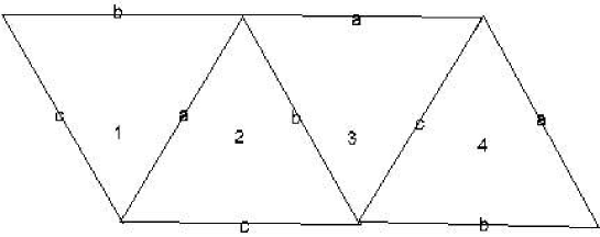
Figure 1. A discretized volume from four triangles
The sides are labelled by the generators

Figure 2. Sequence of gluing

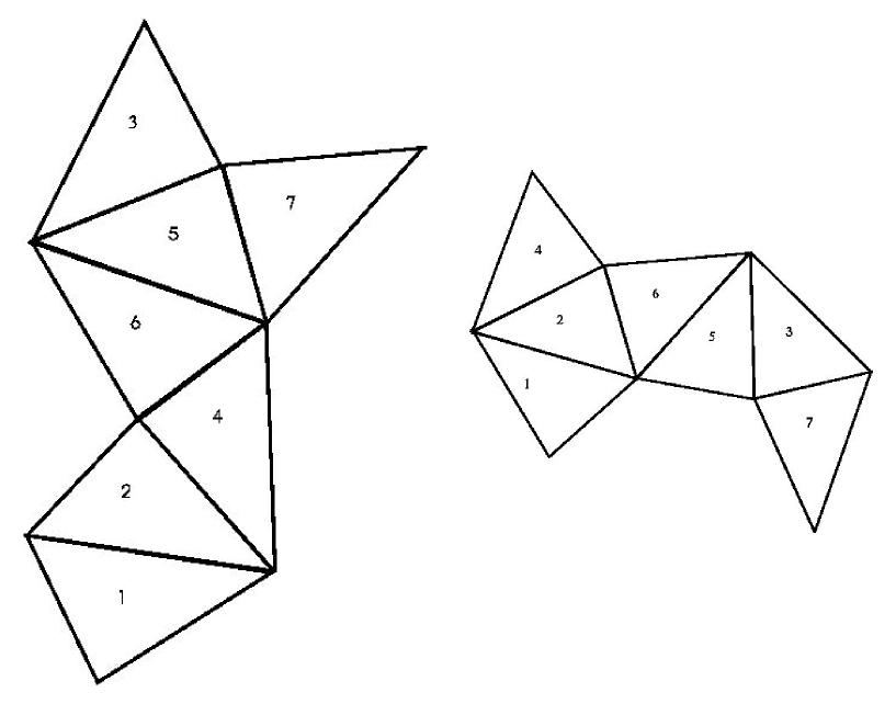
Figure 3. Equivalent volumes from 7 triangles

References

- [1] Aszódi A., Tóth S.: 3D Numerical Model of a Steam Generator Feed Water Valve, V. Nuclear Technique Symposium, 30 November- 1st December 2006, Paks, Hungary
- [2] J. G. Brasseur, Chao-Hsuan Wei: Interscale dynamics and local isotropy in high Reynolds number turbulence within triadic interactions, Phys. Fluids, 6, 842-870 (1994)
- [3] E. J. Caramana, D. E. Burton, M. J. Shashkov, P. P: Whalen: The Construction of Compatible Hydrodynamics Algorithms Utilizing Conservation of Total Energy, J. of Comp. Phys, 146, 227-262 (1998)
- [4] J. M. Hyman, M. Shashkov: Mimetic Discretization for Maxwell’s Equations, J. of Comp. Phys, 151, 881-909 (1999)
- [5] J. H. Mahaffy: Numerics of codes: stability, diffusion, and convergence, Nucl. Eng. and Design, 145, 131-145(1993)
- [6] Gupta, K. K. Development of a finite element aeroelastic analysis capability, Journal of Aircraft, 33 no.5, 995-1002 (1996)
- [7] Vlahopoulos N., Garza-rios L. O., Mollo C. : Numerical implementation, validation, and marine applications of an Energy Finite Element formulation, Journal of ship research, 43, no3, pp. 143-156 (1999)
- [8] H. K. Cho, B. J. Yun, C.-H. Song, G. C. Park: Experimental validation of the modified linear scaling methodology for scaling ECC bypass phenomena in DVI downcomer, Nucl. Eng, Design, 235, 2310-2322 (2005)
- [9] R. Brooks: Constructing Isospectral Manifolds, Am. Math. Monthly, 95, 823-839 (1988)
- [10] J. Stillwell: Classical Topology and Combinatorial group Theory, Springer, New York, 1993, Chapter 8.1
- [11] M. Hamermesh: Group Theory and Its Application to Physical Problems, Argonne National Laboratory, 1962, Addison-Wesley, Reading
- [12] J. Hersch: Erweiterte Symmetrieeigenschaften von Lösungen gewisser linearer- Rand und Eigenwertprobleme, J. für die reine und angewandte Math. 218, 143(1965)
- [13] C. Gordon, D. Webb, S. Wolpert: Isospectral plane domains and surfaces via Riemannian orbifolds, Inventiones mathematicae, 110, 1-22 (1992)
- [14] P. Buser: Isospectral Riemannian Surfaces, Ann. Inst. Fourier, Grenoble, 36, 167-192 (1986)
- [15] C. Gordon: When you Can’t Hear the Shape of a Manifold, The Mathematical Intelligencer, 11, 39-47(1989)
- [16] C. Gordon and D. Webb: You Can’t Hear the Shape of a Drum, American Scientist, 84, 46-55 (1996)
- [17] P. Buser, J. Conway, P. Doyle, K.-D. Semmler: Some planar isospectral domains, Manuscript, (1994)
- [18] P. Bérard: Transplantation et isospectralité I., Math. Ann. 292, 547-559 (1992)
- [19] P. Buser: Cayley Graphs and Planar Isospectral Domains, p. 64-77, in : Sunada, T. (ed.): Geometry and Analysis on Manifolds, Lecture Notes Math. Vol. 1339, Springer, Berlin, (1988)
- [20] T. Sunada: Riemannian coverings and isospectral manifolds, Annals of Mathematics, 121, 169-186 (1985)
- [21] The GAP Group, GAP — Groups, Algorithms, and Programming, Version 4.4.8; 2006 (http://www.gap-system.org)
- [22] M. Makai and Y. Orechwa: Covering group and graph of discretized volumes, Central European Journal of Physics, 2(4), 1-27(2004)
- [23] W. Miller: Symmetries and Separation of Variables, Addison-Wesley, Reading, 1977, Chapter 3.1 and P. J. Olver: Applications of Lie Groups to Differential Equations, Springer, New York, (1986)
- [24] D. Sattinger: Group Theoretic Methods in Bifurcation Theory, Springer, Berlin, 1979
- [25] C. Gordon, E. Makover and D. Webb: Transplantation and Jacobians of Sunada isospectral Riemann surfaces, Advances in Mathematics, 197, 86-119(2005)
- [26] G. Golub and W: Kahan: Calculating the Singular Values and Pseudo- Inverse of a Matrix, SIAM Journal of on Numerical Analysis, Ser. B. 2, 205-224(1965)