Dynamics of small perturbations against a stationary polariton distribution

Abstract

The dynamics of small perturbations against the stationary density matrix of a pumped polariton system with only one photon polarization is studied. Depending on the way the system is pumped and probed, decay times ranging from 30 to 5000 ps are found. The large decay times under resonant pumping are related to a bottleneck effect in the decay of the excess (probe) populations of dark polariton states. No singular behaviour at the threshold for polariton lasing is observed.

Polariton lasers are lasers without population inversion Imamoglu . Coherence buildup in them is the result of the quasibosonic statistics of the polaritons, i.e. quasiparticles composed by electron-hole pairs from a quantum well strongly interacting with photons from a semiconductor microcavity. They share similarities with ordinary photon lasers and Bose-Einstein condensates Deng ; Bajoni . In these devices, the threshold power for lasing is 1 - 2 orders of magnitude lower than in ordinary lasers. Room-temperature polariton lasing has been recently reported Christopoulos .

Besides these promising characteristics, polaritons in microcavities provide an exceptional possibility for fundamental research. An example is the recent paper [Ballarini, ], where the authors seek for evidences of the Goldstone boson, which should appear in connection with the buildup of coherence in the polariton system. Indeed, in a cylindrical microcavity, the two (approximately) circular polarizations of the fundamental photon mode are related to two degenerate polariton “condensates”. The relative phase between the two photon polarizations acts as an order parameter. Phase fixing leads to a linear polarization Kavokin , whose direction can be easily rotated (the Goldstone excitation). In paper Ballarini , Ballarini et. al. study the changes in the PL response of a planar microcavity induced by small pulse perturbations of the pumping. They measure the lifetime of these perturbations, showing that it is much higher than the cavity decay time, and that it increases when the stationary pumping approaches the threshold for polariton lasing. These results are interpreted as a measurement of the lifetime of the Goldstone boson Carusotto .

Recent experimental measurements of time-resolved PL in similar systems bistability reveal the importance of both the dynamics involving a single polarization, and the dynamics involving the two photon polarizations. On the other hand, a system with a single photon polarization - a single polariton condensate - could be realized by means of a strong magnetic field breaking the degeneracy between the “right-handed” and “left-handed” condensates.

In the present paper, I consider a model with a single photon polarization and explore how the way the system is pumped and probed influences the decay dynamics of the perturbations. I started from a scheme, sketched in Refs. [nuestraPRL, ; distortedGibbs, ], in which pumping and photon losses in the polariton system are described by means of two terms in the master equation for the density matrix. The linearization of the master equation around the stationary solution leads to a system of equations with a source term for the small perturbations. The way the system is pumped determines the small-oscillation modes of these equations, whereas the way the system is probed determines which of the eigenmodes are excited. In an oversimplified model, with unrealistic parameters, I found decay times from 30 to 5000 ps, with no singular behaviour at the polariton lasing threshold. The large decay times correspond to eigenmodes involving the excitation of dark polariton states which, under resonant pumping, exhibit a bottleneck effect.

The starting point is a simple expression for the stationary spectral function, $S(\omega)$, describing the PL emission along the cavity symmetry axis, Eq. (19) of Ref. laser, :

$$S(\omega)=\frac{1}{\pi}\sum_{I,J}\frac{|\langle I|a|J\rangle|^{2}\rho_{J}^{(\infty)}~{}\Gamma_{IJ}}{\Gamma_{IJ}^{2}+(\omega_{IJ}-\omega)^{2}}.$$ (1)

The magnitudes $\Gamma_{IJ}$ (linewidhts) and $\omega_{IJ}=(E_{J}-E_{I})/\hbar$ depend only on the many-polariton wavefunctions and energies, and the system parameters, $P$ (pumping rate), and $\kappa=0.1~{}{\rm ps}^{-1}$ (photon losses rate). $\langle I|a|J\rangle$ are the matrix elements of the photon annihilation operator between the many-polariton wavefunctions $|J\rangle$ and $|I\rangle$.

In our model, describing a many-exciton quantum dot strongly interacting with the lowest photon mode of a microcavity laser , the wavefunctions and energies, and from them $\Gamma_{IJ}$, $\omega_{IJ}$, and $\langle I|a|J\rangle$, are obtained by numerically diagonalizing the electron-hole-photon Hamiltonian. On the other hand, the stationary solutions, $\rho_{I}^{(\infty)}$ should be obtained from the master equation for the occupations (coherences are three orders of magnitude smaller distortedGibbs and will be neglected):

$$\frac{{\rm d}\rho_{I}}{\rm dt} = \kappa\sum_{J}|\langle I|a|J\rangle|^{2}\rho_{J}-\kappa~{}\rho_{I}\sum_{J}|\langle J|a|I\rangle|^{2}$$ (2)

$$+ \sum_{N_{pol}(J)=N_{pol}(I)-1}\rho_{J}~{}P_{JI}$$

$$- \rho_{I}\sum_{N_{pol}(J)=N_{pol}(I)+1}P_{IJ}.$$

$N_{pol}(J)$ is the polariton number (number of electron-hole pairs plus number of photons, which is a conserved quantity) of state $|J\rangle$, and $P_{JI}$ is the pumping rate from state $J$ to state $I$. Notice that Eqs. (2) depends only on $\kappa$, $P$, and the matrix elements $\langle I|a|J\rangle$. These equations are linearly dependent, which expresses the conservation of probability:

$$\sum_{I}\rho_{I}=1.$$ (3)

The stationary solutions, $\rho_{I}^{(\infty)}$, are obtained by making the l.h.s. of Eqs. (2) equal to zero, and complementing this homogeneous linear system with the normalization condition, Eq. (3).

Under a small perturbation of the pumping rate, $\delta P(t)$, there is a variation of the density matrix, $\delta\rho(t)$, and a variation of the spectral function:

$$\delta S(\omega,t)=\frac{1}{\pi}\sum_{I,J}\frac{|\langle I|a|J\rangle|^{2}~{}\delta\rho_{J}(t)~{}\Gamma_{IJ}}{\Gamma_{IJ}^{2}+(\omega_{IJ}-\omega)^{2}}.$$ (4)

The response, $\delta\rho_{I}$, to the pulsed perturbation $\delta P(t)$ satisfies the linear system obtained by varying Eqs. (2):

$$\frac{{\rm d}\delta\rho_{I}}{\rm dt} = \kappa\sum_{J}\left\{|\langle I|a|J\rangle|^{2}\delta\rho_{J}-|\langle J|a|I\rangle|^{2}\delta\rho_{I}\right\}$$ (5)

$$+ \sum_{N_{pol}(J)=N_{pol}(I)-1}\left(\delta\rho_{J}~{}P_{JI}+\rho_{J}^{(\infty)}\delta P_{JI}(t)\right)$$

$$- \sum_{N_{pol}(J)=N_{pol}(I)+1}\left(\delta\rho_{I}P_{IJ}+\rho_{I}^{(\infty)}\delta P_{IJ}(t)\right),$$

which should be complemented with:

$$\sum_{I}\delta\rho_{I}=0.$$ (6)

The structure of Eqs. (5) is the following: ${\rm d}\delta\rho/{\rm dt}=A\delta\rho+\delta P(t)B\rho^{(\infty)}$. The eigenvalues of matrix $A$ are the small oscillation frequencies of the system, whereas the probe perturbation, matrix $B$, and the stationary density matrix conform the source term determining which oscillation modes are excited by the probe pulse.

Let us recall the diagonal terms in Eqs. (5) in order to get a qualitative understanding of the decay times:

$$\frac{{\rm d}\delta\rho_{I}}{\rm dt} = -\kappa\sum_{J}|\langle J|a|I\rangle|^{2}\delta\rho_{I}$$ (7)

$$- \delta\rho_{I}\sum_{N_{pol}(J)=N_{pol}(I)+1}P_{IJ}+\cdots$$

This equation shows that the excess occupation of state $I$, $\delta\rho_{I}$, can decay in two ways. The first term corresponds to photon emission, and the second to pumping the excess occupation to a higher polariton state, $J$, which may further decay through photon emission. When the state $I$ is dark, $\sum_{J}|\langle J|a|I\rangle|^{2}\approx 0$, only the second mechanism acts. If, in addition, $\delta\rho_{I}$ is not pumped to higher states because of selective pumping ($P_{IJ}\approx 0$), then the decay of $\delta\rho_{I}$ may take very long times. Below, we consider different regimes of pumping and probing the polariton system.

Figure 1: Uniform pumping. (a) Position of the PL line as a function of the pumping rate. (b) Photon second-order coherence function.

(a) Uniform pumping and uniform perturbation

In this case, $P_{IJ}=P$, and $\delta P_{IJ}(t)=\delta P(t)$. This situation seems to correspond to laser excitation energies well above the lower polariton branch, and perturbations at these higher energies.

I show in Fig. 1 the position of the main PL line as a function of the pumping rate, and the corresponding photon second-order coherence function, $g^{(2)}(0)$. The jump in the position of the line, and the values near one of $g^{(2)}(0)$ identify the threshold for polariton lasing at $P_{thr}\approx 0.00014$ ps^-1 in the model, where I use the following states in order to solve Eqs. (2) for the stationary density matrix: the vacuum ($I=1$), the 17 existing one-polariton states in the model ($I=2-18$), the 256 existing two-polariton states ($I=19-274$), and 256 states in each sector with $2<N_{pol}\leq 10$.

I will study the decay dynamics of the probe for $P$ values in the vicinity of $P_{thr}$. The probe pulse is taken in the following way:

$$\delta P(t)=10^{-5}\exp-(t-1)^{2}~{}{\rm ps}^{-1},$$ (8)

where $t$ is given in ps. We find the $\delta\rho_{I}$ from Eqs. (5) and compute, as in the experiment Ballarini , the energy-integrated differential PL response:

$$\delta S(t)=\sum_{J}\delta\rho_{J}(t)\sum_{I}|\langle I|a|J\rangle|^{2}.$$ (9)

The sum over $I$ is restricted to states such that $|E_{J}-E_{I}-E_{ref}|<\delta E$, where $\delta E=2$ meV, and the reference energy in the present case is $E_{ref}=1489.2$ meV.

I draw in Fig. 2 (a) the computed $\delta S(t)$ for three values of the pumping rate. They show characteristic decay times of around 30 ps. These values can be understood from the eigenvalues of the linearized decay modes. Indeed, let us write the smallest (in absolute value) eigenvalues in the present case: …, -0.0358, -0.0287, -0.0117, -0.0067, -0.0023 ps^-1. Notice that they are real, i.e. purely decaying (non propagating) modes. The first of them (-0.0358 ps^-1, decay time $\sim 28$ ps, there are many such eigenvalues) corresponds basically to an eigenvector in which a single dark one-polariton state is excited. The decay is due to pumping to two-polariton states with further emission of photons. Notice that $P_{thr}=0.00014$ ps^-1 times the number of available two-polariton states (256) is equal roughly to the eigenvalue, -0.0358 ps^-1. These are the modes dominating the observed behaviour of $\delta S(t)$ in the present case. Let us stress that the eigenvalues practically do not change when $P$ is varied around $P_{thr}$. Thus, we can not relate the slowest mode (or any other) to the lasing transition. In the scheme of perturbation I am using, modes with larger decay times are not excited. In particular, the last one (-0.0023 ps^-1, decay time $\sim 434$ ps) corresponds to an eigenvector involving the simultaneous excitation of one- and two-polariton dark states combined with higher polariton states. We shall see that slower decaying modes can be observed by means of a selective excitation.

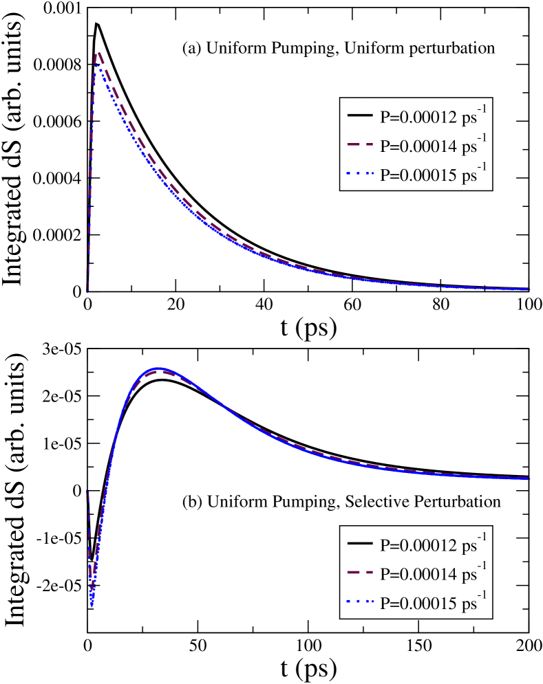
Figure 2: (Color online) Time evolution of the energy-integrated differential PL response, Eq. (9), under uniform pumping. (a) Uniform perturbation. (b) Selective perturbation.

(b) Uniform pumping, selective perturbation

At this point I consider a situation in which the system is pumped at high energies, as above, but resonantly perturbed. This means that $\delta P_{IJ}(t)$ is given by Eq. (8), only when the energy difference satisfies the inequality $|E_{J}-E_{I}-E_{perturb}|<\delta E$. Otherwise it is zero. We show results for $E_{perturb}=1499.25$ meV, and $\delta E=2$ meV. The chosen $E_{perturb}$ corresponds to the resonant excitation of a dark one-polariton state, labeled by the number 15 ($E_{perturb}=E_{15}-E_{1}$). Of course, other transitions may have the same, or close, excitation energy, and could be excited if they satisfy the above inequality. Below, we shall discuss in more details, how a dark state could be perturbed.

The eigenvalues have not changed because I have not modified the pumping scheme. But the energy-integrated $\delta S(t)$ shows decay times of around 60 ps in the present case, indicating the excitation of slower-decaying modes, as compared to uniform perturbation. Results are drawn in Fig. 2 (b), where an oscillation at early times is also observed. It is possible that with a different perturbation energy, $E_{perturb}$, or a different perturbation strategy the slowest mode could be reached as well.

Figure 3: Selective pumping. (a) Position of the PL line as a function of the pumping rate. (b) Photon second-order coherence function.

(c) Selective pumping, selective perturbation

Finally, we consider resonant pumping. Selective pumping can increase dramatically the decay times because there could be almost dark states, not connected to higher states through pumping. The decay of an excess occupation in these states could take very long times.

The stationary pumping rate is chosen in the form: $P_{IJ}=P$ only when $|E_{J}-E_{I}-E_{pump}|<\delta E$, where $E_{pump}=1488$ meV, and $\delta E=2$ meV. The position of the main PL line and the photon second-order coherence function are shown in Fig. 3. The jump in the position of the PL line and the abrupt variation of $g^{(2)}(0)$ allow us to identify the threshold rate: $P_{thr}\approx 0.04$ ps^-1. Notice that this value is much higher than the threshold under uniform pumping, something reasonable. Notice also that even below threshold the coherence function take values very close to one. This initial coherence is, in some sense, inherited from the pumping.

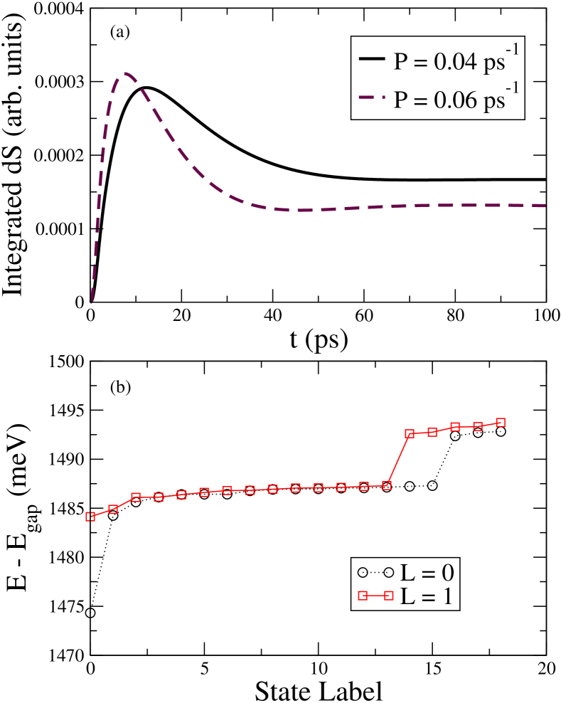
Figure 4: (Color online) (a) Time evolution of the energy-integrated differential PL response under selective (resonant) pumping and selective perturbation. (b) The lowest 2-polariton states with $L=0$ and $L=1$.

The energy-integrated PL response is drawn in Fig. 4 (a) for $P=0.04$ and $P=0.06$ ps^-1. After an initial transient period, the curves become almost flat, suggesting the excitation of very slow decay modes. There are many eigenvalues of the linearized problem with absolute value lower than 0.01 ps^-1 (decay times larger than 100 ps). The smallest of them is -0.0002 ps^-1, that is a decay time of 5000 ps. Let us stress that no singular behaviour of the eigenvalues across the threshold is found, which means that we can not relate any of the eigenmodes to the lasing threshold.

Let us consider the question about the selective (resonant) pumping or perturbation of a dark state. Electron-hole pairs with a definite energy could be injected to the system, but this seems to be difficult to control. On the other hand, the direct optical transition is prohibited because, by definition, the state is dark. However, notice that we are considering transitions between $L=0$ states laser , which are responsible for the PL emission along the cavity symmetry axis. States with $L=1$ or higher, very close in energy to $L=0$ states, are very common, as can be seen, for example, in Fig. 4(b). These $L=1$ states could be optically excited (with a non-zero transferred linear momentum, $\vec{k}$), and then may decay towards $L=0$ states through emission of very low-energy acoustical phonons. In the reported experiment Ballarini , the system is both pumped and perturbed by using $\vec{k}\neq 0$ laser beans.

In conclusion, we studied a model polariton system with a single photon polarization and computed decay times of probe pulses against a stationary polariton distribution. Under non-resonant pumping conditions, the computed decay times are 30-60 ps, whereas under resonant pumping very large decay times, of the order of thousands of picoseconds, are obtained. The dark polariton states play a fundamental role in the decay dynamics, specially under resonant pumping, where the excess (probe) occupations of particular dark states may take very long times to decay. No singular behaviour of any decay mode at the threshold for lasing is observed.

This work was supported by the Programa Nacional de Ciencias Basicas (Cuba) and the Caribbean Network for Quantum Mechanics, Particles and Fields (ICTP). The author is grateful to Alejandro Cabo and Alexey Kavokin for discussions.

References

- (1) A. Imamoglu, R.J. Ram, S. Pau, and Y. Yamamoto, Phys. Rev. A 53, 4250 (1996).
- (2) H. Deng, G. Weihs, D. Snoke, J. Bloch, and Y. Yamamoto, Proc. Natl. Acad. Sci. 100, 15318 (2003).
- (3) D. Bajoni, P. Senellart, A. Lemaitre, and J. Bloch, Phys. Rev. B 76,201305 (R) (2007).
- (4) S. Christopoulos, G. Baldassarri Hoger von Hogersthal, A.J.D. Grundy, et. al., Phys. Rev. Lett. 98, 126405 (2007).
- (5) D. Ballarini, D. Sanvitto, A. Amo, et. al., Phys. Rev. Lett. 102, 056402 (2009).
- (6) J. Kasprzak, R. Andre, Le Si Dang, et. al., Phys. Rev. B 75, 045326 (2007).
- (7) M. Wouters and I. Carusotto, Phys. Rev. B 75, 075332 (2007).
- (8) A.A. Demenev, A.A. Shchekin, A.V. Larionov, S.S. Gavrilov, and V.D. Kulakovskii, Phys. Rev. B 79, 165308 (2009).
- (9) H. Vinck-Posada, B.A. Rodriguez, P.S.S. Guimaraes, A. Cabo, and A. Gonzalez, Phys. Rev. Lett. 98, 167405 (2007).
- (10) C.A. Vera, A. Cabo, and A. Gonzalez, Phys. Rev. Lett. 102, 126404 (2009).
- (11) C.A. Vera, H. Vinck-Posada, and A. Gonzalez, arXiv:0807.1137v2.