Breakdown of large-N reduction in the quenched Eguchi-Kawai model

Abstract:

We study the validity of the large-N equivalence between four-dimensional SU(N) lattice gauge theory and its momentum quenched version—the Quenched Eguchi-Kawai (QEK) model. We have found strong evidence that this equivalence does not hold in the weak-coupling regime (and thus in the continuum limit). This is based on weak-coupling analytic arguments and Monto-Carlo simulations at intermediate couplings with $20\leq N\leq 200$. Since detailed expositions of our arguments, methods and results have already appeared in Phys. Rev. D78:034507 (2008) and Phys. Rev. D78:074503 (2008), we attempt here to give a more intuitive explanation of our results. The breakdown of reduction that we find is due to a dynamically generated correlation between different Euclidean components of the gauge fields.

1 Introduction

QCD simplifies in the ’t Hooft limit of a large number of colors, and as a result it has been a long-standing goal to understand the properties of the theory in that limit [1], including on the lattice [2]. In this paper we reconsider an alternative to conventional large volume simulations, namely the use of large-$N$ volume reduction to single-site models [3, 4, 5, 6] (see also the related Ref. [7]). This allows one, in principle, to study very large values $N\sim O(100-400)$ with modest resources. In this paper we choose to study one of the variants of the original Eguchi-Kawai (EK) volume reduction, namely the quenched Eguchi-Kawai (QEK) model. Our motivation is two-fold: First, it is the only single-site model whose equivalence with large-$N$ QCD has yet to be thrown in doubt (in contrast to twisted Eguchi-Kawai model—see Refs. [8]); Second, we use it as a tool to gain experience with single-site large-$N$ models, before turning to the theory with adjoint fermions [6].

Since a detailed discussion of this work, including a full list of relevant references, has already appeared [9], we use this opportunity to give a less technical and more intuitive presentation.

2 A brief review of the EK and QEK models

The $U(N)$ EK model of Ref. [3] is a matrix model whose connected correlation functions are expected to have, under certain assumptions, the same large-$N$ limits as appropriately chosen correlation functions in a $U(N)$ pure gauge theory. It is a specific example of an orbifold projection mapping a “mother” theory (the gauge theory in our case) to a “daughter” theory (here the matrix model), that, under certain conditions, becomes an equivalence in the large-$N$ limit. This equivalence applies only to “neutral sectors” of the two theories, which consist of correlation functions invariant under translations in the gauge theory, and invariant under the $U(1)^{d}$ “center” symmetry in the matrix model [10] ($d$ is the number of space-time dimensions). Obtaining the reduced model from the gauge theory is easy: one simply sets to zero all Fourier components of the gauge fields except for the zero mode and so performs the mapping $U_{\mu}(x)\to U_{\mu}$. Substituting this into the pure gauge Wilson action gives the partition function of the EK model, a single-site lattice gauge theory:

$$Z_{EK}=\int DU\,\exp(-{S_{EK}})\,,\qquad S_{EK}=-Nb\sum_{\mu<\nu}2{\rm Re}\,{\rm Tr}\,(U_{\mu}U_{\nu}U_{\mu}^{\dagger}U_{\nu}^{\dagger})\,.$$ (1)

The essence of large-$N$ reduction is that vacuum expectation values (VEVs) of neutral operators that map into each other have coinciding large-$N$ limits. For this to hold the vacuum has to be invariant under the symmetries defining the projection, for otherwise the desired expectation values do not lie in the neutral sectors. Indeed the original EK paper [3] focused on center-invariant VEVs of Wilson loops projected to zero momentum. Assuming implicitly that translation invariance is unbroken in the gauge theory, while stressing explicitly that the center symmetry must remain intact in both the gauge theory and matrix model, the authors proved that these VEVs become equal to corresponding quantities in the matrix model at large-$N$. (Technically, they showed that the Dyson-Schwinger equations obeyed by Wilson loops in the two theories coincide.)

Unfortunately, the vacuum of the EK model was shown to spontaneously break its center symmetry for weak enough bare lattice coupling if $d>2$ [4, 11, 12]. Consequently, the EK model does not reproduce the neutral sector of large-$N$ QCD. Initially this was seen in the weak-coupling limit by analyzing the effective potential, $V_{\rm eff}$, felt by the eigenvalues of the link matrices $U_{\mu}$ [4]. The eigenvalues are attracted, leading to a ground state with $U_{\mu}$ proportional to the identity up to a phase, which spontaneously breaks the center symmetry. To overcome this they suggested quenching the eigenvalues, thereby defining a new prescription for calculating neutral-sector expectation values, $\langle{\cal O}\rangle_{\rm quenched}$. This prescription has two parts:

1. Calculate $\langle{\cal O}\rangle_{p}$ for a frozen set of eigenvalues: ${\rm Eig}(U_{\mu})=e^{ip^{\mu}_{a}}\,;\ a=1,2,\dots,N$. Here $\langle,\rangle_{p}$ denotes an average with an action obtained from Eq. (1) by freezing the fluctuations in the eigenvalues of $U_{\mu}$. This means writing $U_{\mu}=V_{\mu}\,e^{ip^{\mu}}\,V^{\dagger}_{\mu}$, with $p^{\mu}={\rm diag}(p_{1}^{\mu},\dots,p_{N}^{\mu})$ the frozen eigenvalues and $V_{\mu}\in U(N)$, and replacing $DU_{\mu}$ with $DV_{\mu}$.

2. Average over the $p^{a}_{\mu}$ with a measure $d\,\mu(p)$ that is both $U(1)^{d}$ invariant and distributes each of the $p_{a}^{\mu}$ uniformly and independently over $[0,2\pi)$ when $N\to\infty$:
   $\langle{\cal O}\rangle_{\rm quenched}\equiv\int\,\prod_{a,\mu}d\mu(p_{a}^{\mu})\,\langle{\cal O}\rangle_{p}$.

We stress that this prescription differs substantially from the ordinary way one calculates expectation values in field theory. In particular, for the quenched prescription to coincide with an ordinary field theory average one would need to use $d\mu(p)\propto\prod_{a,\mu}dp_{a}^{\mu}e^{-V_{\rm eff}(p)}$ [13]. This is a highly non-uniform measure over the eigenvalues, as noted above. By removing the $V_{\rm eff}$ factor, e.g. by using the uniform measure $d\mu(p)\propto\prod_{a,\mu}dp_{a}^{\mu}$, one expects the center symmetry to remain unbroken.

It is illuminating to understand the quenching prescription in a different way [4, 14, 15]. The approach is first formulated for two-index scalar fields. For example, one can define a mapping between the large-volume theory with $N\times N$ adjoint fields $\phi(x)$ and a theory of $N\times N$ matrices $\widetilde{\phi}$: $\phi^{ab}(x)\to e^{i\sum_{\mu}(p_{a}-p_{b})^{\mu}\,x_{\mu}}\,\widetilde{\phi}^{ab}$. Here $a,b$ are color indices, $x_{\mu}$ is the space-time coordinate, and $p_{a}^{\mu}$ are predefined variables which are referred to as momenta for a reason that will become clear below. Substituting this mapping into the field theory action and observables yields the matrix model, whose expectation values depend on the $p_{1,2,\dots,N}^{\mu}$. Next, one is instructed to integrate such expectation values over $p$. Under certain assumptions, the result will become equal, when $N\to\infty$, to the corresponding expectation values in the field theory.

This equality can be shown to any order in perturbation theory (perturbing in, say, the three-point coupling of the scalar theory) [15]. At large $N$, planar diagrams dominate. For such diagrams, one finds that, prior to the $p$ integral, the perturbative expression in the matrix model at a given order coincides with the momentum space integrand of the corresponding Feynman diagram in the field theory. In this correspondence the momentum $q^{\mu}$ of the field $\phi^{ab}(q)$ is given by the difference $q_{ab}^{\mu}\equiv p_{a}^{\mu}-p_{b}^{\mu}$ in the matrix model. The $p$ integration can then be identified as being over the momenta flowing in the planar diagrams, and one recovers the field theory integral.

Thus the two steps in the quenching prescription can be thought of as (1) calculating the contribution to an expectation value $\langle{\cal O}\rangle_{p}$ of a point $p^{\mu}$ at a Euclidean Brillouin Zone, and (2) integrating over the Brillouin zone uniformly to get the full $\langle{\cal O}\rangle_{\rm quenched}$. This way of embedding space-time (or rather its first Brillouin zone) into index space is typical of volume reduced models and was already noted in Refs. [4, 13].

Performing the mapping in a lattice gauge theory, so that $\phi^{ab}(x)$ becomes $U^{ab}_{\mu}(x)$, one obtains a matrix model with an action similar to that in Eq. (1), but with $U_{\mu}$ replaced by $U_{\mu}\,e^{ip^{\mu}}$. The momentum factor $e^{ip^{\mu}}$ can, however, be absorbed by a change of variables, so one ends up back at the problematic EK model. Various approaches have been used to avoid this problem. Refs. [14] restrict their study to $O(N)$ models, while Refs. [15, 16] change the measure of the path integral:

1. Ref. [15]: $\int_{U(N)}DU_{\mu}\to\int_{U(N)}DU_{\mu}\,\int_{U(N)}DV_{\mu}\,\delta(U_{\mu}e^{ip^{\mu}}-V_{\mu}\,e^{ip^{\mu}}V^{\dagger}_{\mu})$ (up to $p$-dependent terms), thus forcing the eigenvalues of $U_{\mu}e^{ip^{\mu}}$ to be $e^{ip^{\mu}_{a}}$. Intuitively, $U_{\mu}$ is being forced to fluctuate around unity, so that absorbing $p^{\mu}$ into $U_{\mu}$ is impossible. Note that the integral over $V_{\mu}$ could equally well be over the coset $U(N)/U(1)^{N}$ in which multiplication from the right by a $U(1)^{N}$ matrix is divided out.

2. Ref. [16]: $\int_{U(N)}DU_{\mu}\to\int_{U(N)/U(1)^{N}}DU_{\mu}$ (together with a gauge-fixing term). Here one restricts the integration regime to the coset such that $U_{\mu}$ cannot absorb the $e^{ip^{\mu}}$ factor.

The first prescription is, in fact, identical to the QEK model of Ref. [4], as can be seen by using the $\delta-$functions to perform the $U$ integrations [15]. The second prescription is different and we call it the DW model. An obvious advantage of the QEK over the DW model is that the “reduced” $U(N)$ gauge invariance $U_{\mu}e^{ip^{\mu}}\to\Omega U_{\mu}e^{ip^{\mu}}\Omega^{\dagger}$ is realized in the QEK model as $V_{\mu}\to\Omega V_{\mu}$. By contrast, the DW model has no gauge symmetry: if one writes $\Omega U_{\mu}e^{ip^{\mu}}\Omega^{\dagger}=U^{\prime}_{\mu}e^{ip^{\mu}}$ then, in general, $U^{\prime}_{\mu}\notin U(N)/U(1)^{N}$. Indeed, the DW model is defined including gauge-fixing so as to avoid this problem [16]. This means that a numerical study of the DW model appears quite nontrivial.

Let us restate in another way why one needs to change the measure of the path integral over the $U_{\mu}$. In the weak coupling regime, $b\to\infty$, configurations close to the minima of the action dominate. To avoid the symmetry-breaking of the EK model, one wants there to be a single minimum (up to gauge transformations). For the action (1) with $U_{\mu}$ replaced with $U_{\mu}e^{ip^{\mu}}$, however, there are multiple minima, occurring when the $U_{\mu}e^{ip^{\mu}}$ in all directions are arbitrary diagonal matrices (up to gauge transformations). By changing the measure as in Refs. [15, 16] one aims to make the only minimum available that at $U_{\mu}=1$. This is indeed what happens, by construction, in the DW model. One might expect the same for the QEK model: the action is minimized when $V_{\mu}\,e^{ip_{\mu}}\,V^{\dagger}_{\mu}\in U(1)^{N}$ (up to gauge transformations), and this condition is satisfied by $V_{\mu}=1$. This, however, is not the whole story: as has long been known, there are other solutions to this equation given by $V_{\mu}=P_{\mu}$ with $P_{\mu}$ a $U(N)/U(1)^{N}$ matrix that, when conjugating $e^{ip_{\mu}}$, gives rise to a permutation of the color indices of $p^{a}_{\mu}$. These minima are nonperturbative ($P_{\mu}$ is very far from the unit matrix) and we find that they play a central role in the (in)validity of large-$N$ quenched reduction.

We began this section by describing reduction as an example of the orbifolding paradigm. Once one quenches the daughter theory, however, this paradigm does not apply in a straightforward way. This is because VEV’s in the daughter QEK model are calculated in a way that separates the gauge fields into quenched and unquenched degrees of freedom—a separation that is absent from the mother gauge theory. Nonetheless, an argument for quenched reduction has been given using the Dyson-Schwinger equations for Wilson loops [15]. These “loop equations” are different in the gauge theory and QEK model, but the differences are proportional to quenched expectation values of center-invariant quantities composed of center non-invariant Wilson loops. An example of such a quantity is $\langle|W_{C}|^{2}\rangle_{\rm quenched}$, where $W_{C}$ is center non-invariant. Reduction can hold only if such quantities vanish as $N\to\infty$. They will vanish if quenched expectation values factorize, for then $\langle|W_{C}|^{2}\rangle_{\rm quenched}=|\langle W_{C}\rangle_{\rm quenched}|^{2}+O(1/N)$, and the enforcement of center-symmetry in the QEK implies that $|\langle W_{C}\rangle_{\rm quenched}|=0$. The crucial question is thus whether factorization holds for quenched expectation values.

3 (In)Validity of large-$N$ quenched reduction

In this section we discuss analytic, weak-coupling considerations that extend those presented in Refs.[4] and [11] to include the effects of the multiple classical minima which, as discussed above, come in the form of permutations of the $p_{a}^{\mu}$. To be precise, the minima are $U^{\rm min}_{\mu}e^{ip^{\mu}}=V^{\rm min}_{\mu}\,e^{ip^{\mu}}\,V^{{\dagger},{\rm min}}_{\mu}=e^{i\widetilde{p}^{\mu}}$, with $\widetilde{p}_{a}^{\mu}=p_{\sigma(a)}^{\mu}$ and $\sigma(a)$ one of the $N!$ permutations of the indices $a$. Here we describe how this classical degeneracy is removed by quantum fluctuations, with the resulting ground state corresponding to a certain permutation which is unrelated to the original choice of $p_{a}^{\mu}$. This, by itself, is a strong indication for the breakdown of quenched large-$N$ reduction, since it invalidates the idea that for each value of $p^{\mu}$, the value of $\langle{\cal O}\rangle_{p}$ is the contribution of a point corresponding to $p^{\mu}$ in the Brillouin zone.

To show how quantum fluctuations remove the classical degeneracy we minimize the effective potential $V_{\rm eff}$ over the space of all permutations of the color indices of the input momenta $p_{a}^{\mu}$ (with permutations in different directions being independent). For brevity, we consider here the case where the $N$ momenta in each direction, $p_{a}^{\mu}$, are always a permutation of the “clock” momenta $p_{a}^{\rm clock}\equiv 2\pi a/N$. The situation for other distributions of momenta is similar, as discussed in Refs. [9]. For clock momenta we find that, for $d\geq 3$, the minimum of $V_{\rm eff}$ occurs for permutations in which the momenta in all directions are ordered similarly. In equations, the statement is that $\widetilde{p}_{a}^{\mu}-\widetilde{p}_{a}^{\nu}=\alpha^{\mu\nu}$ for all $a$, and we refer to this as “locking” of the momenta. There is thus an overall shift between different Euclidean directions, whose value is an arbitrary clock momentum that can depend on $\mu$ and $\nu$, but which is independent of the color index. This implies that the difference $q_{ab}^{\mu}=\widetilde{p}_{a}^{\mu}-\widetilde{p}_{b}^{\mu}$, which we recall plays the role of the gluon momentum in Feynman diagrams, is independent of $\mu$. This in turn means that instead of integrating over the full Brillouin zone (as would be the case if the $p^{\mu}$ in different directions were independent) one is effectively integrating along the diagonal of the Brillouin zone, i.e. over a one-dimensional line!

It is useful to have order parameters that can detect such “locking”, and a simple choice is the center-non-invariant reduced Wilson loops $M_{\mu,\nu}\equiv\frac{1}{N}\,{\rm tr}\,\,U_{\mu}\,U_{\nu}$ and $M_{\mu,-\nu}\equiv\frac{1}{N}\,{\rm tr}\,\,U_{\mu}\,U^{\dagger}_{\nu}$. Indeed, when the locked ordering takes place one finds that $M_{\mu,-\nu}=e^{i\alpha^{\mu\nu}}$, while $M_{\mu,\nu}=0$. By contrast, if no ordering takes place and all $p_{a}^{\mu}$ are random permutations of $p^{a}_{\rm clock}$, then $M_{\mu,\pm\nu}\sim O(1/N)$. In Fig. 1 we show the dependence, in $d=4$, of $V_{\rm eff}$ on the combined order parameter $M=\frac{1}{2}\sum_{\mu}\,\left(|M_{\mu,\nu}|+|M_{\mu,-\nu}|\right)$, where we have used a Monte-Carlo (MC) to sample permutations. One sees that $V_{\rm eff}$ has a minimum at the “fully locked” ground state with $M=6$, with states having little locking ($M\ll 1$) having a free energy of $O(N^{2})$ higher.

 

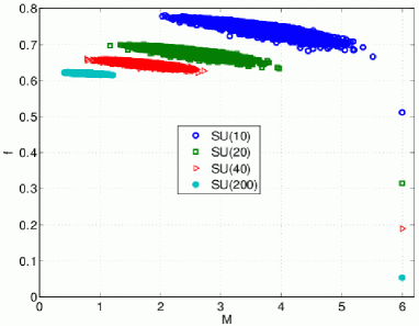
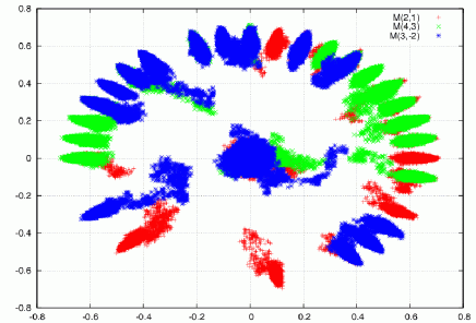
Figure 1: Right panel: The dependence of $V_{\rm eff}/N^{2}$ on the combined order parameter $M$ for random permutations of the clock momenta and for various values of $N$. Left panel: Scatter plot of the values of three chosen $M_{\mu\nu}$’s in a run for $N=40$ and ‘clock’ momenta. We refer to [9] for technical details.

We now come to a crucial observation: if locked ordering occurs then large-$N$ factorization breaks down in the quenched theory. To see this, recall that the quenched prescription instructs us to integrate over the $p_{a}^{\mu}$ in a center-symmetry invariant way. Performing a center transformation on the $p_{a}^{\mu}$ ($p_{a}^{\mu}\to p_{a}^{\mu}+\theta_{\mu}$) will lead to a center-transformed locked vacuum, since the action is center invariant. In this transformed vacuum, $\alpha^{\mu\nu}\to\alpha^{\mu\mu}+\theta_{\mu}-\theta_{\nu}$, so the phase of the $M_{\mu,\nu}$ is shifted. Integrating over the $\theta_{\mu}$, which is part of the integration over the $p_{a}^{\mu}$, will thus lead to the vanishing of the order parameters, e.g. in the example above, $\langle M_{\mu,-\nu}\rangle_{\rm quenched}\simeq\int_{0}^{2\pi}d\alpha^{\mu\nu}\,e^{i\alpha^{\mu\nu}}=0$. By contrast, if one calculates $\langle|M_{\mu,-\nu}|^{2}\rangle_{\rm quenched}$, the phase $\alpha^{\mu\nu}$ cancels, and so $\langle|M_{\mu,-\nu}|^{2}\rangle_{\rm quenched}\sim O(1)\neq|\langle M_{\mu\nu}\rangle_{\rm quenched}|^{2}$. This invalidates large-$N$ factorization in the quenched theory, which, as noted above, implies that the gauge theory and QEK model have different loop equations, and so reduction fails.

The argument for locked ordering described above was perturbative. To check whether it occurs beyond perturbation theory we performed a detailed numerical study of the QEK model at intermediate and strong couplings using MC techniques for $20\leq N\leq 200$. We do not discuss any particulars of these calculations here, referring instead to Refs. [9] (the second reference includes an appendix describing the update algorithms we used, which are nontrivial since the model is quartic in the updated fields).

In our numerical studies we measure the order parameters $M_{\mu\nu}$ in the intermediate coupling regime, and find clear evidence for correlations in the eigenvalue orderings. For example, in the right panel of Fig. 1 we show a typical scatter plot of data obtained for $M_{2,1}$, $M_{4,3}$, and $M_{3,-2}$. This combines results from 20 independent input choices of the $p_{a}^{\mu}$, all being random permutations of $p_{a}^{\rm clock}$. What we see from the figure is that each of these $20$ MC simulations settled into a different vacuum characterized by a distinct value for the phase $\alpha^{\mu\nu}$ of $M_{\mu\nu}$. This is precisely what one expects when locking of the eigenvalue ordering occurs.

We have also obtained direct evidence for the breakdown of large-$N$ reduction: there are large discrepancies between the plaquette values and the structure of the phase diagram of the QEK model and the large-$N$ gauge theory [9]. We have checked that these conclusions are insensitive to the precise form of the quenched eigenvalue distribution, $d\mu(p)$, and to the way we perform the quenched average. We also considered values of $N$ up to $200$ to look for a late onset of $1/N$ behavior, but find none. Therefore we conclude that the momentum quenched large-$N$ reduction of $SU(N)$ lattice gauge theories fails in the weak-coupling regime and thus in the continuum limit.

4 Possible future directions

Our result, together with those of Refs. [8], imply that the only known single-site models that can reproduce the properties of QCD at large-$N$ are the following: (I) The “deformed” Eguchi Kawai of Ref. [17]; (II) the single-site obtained by adding adjoint fermions to the Eguchi-Kawai model [6]; and (III) the momentum quenched model of DW [16]. For a brief discussion on the first two we refer to Refs. [9]. As far as we know, the third alternative has never been explored nonperturbatively; its obvious advantage over the standard type of momentum quenching is that its path integral has a unique minimum in weak coupling, with no difficulties related to permutations. As mentioned above, however, this model involves gauge fixing and so it is clearly more involved to study numerically. We leave the exploration of all these single-site models to future studies.

References

- [1] G. ’t Hooft, Nucl. Phys. B 75, 461 (1974); E. Witten, Nucl. Phys. B 160, 57 (1979); A. V. Manohar, arXiv:hep-ph/9802419. For a recent review see K. Peeters and M. Zamaklar, arXiv:0708.1502 [hep-ph].
- [2] M. Teper, [arXiv:hep-lat/0509019]; R. Narayanan and H. Neuberger, arXiv:0710.0098 [hep-lat].
- [3] T. Eguchi and H. Kawai, Phys. Rev. Lett. 48, 1063 (1982).
- [4] G. Bhanot, U. M. Heller and H. Neuberger, Phys. Lett. B 113, 47 (1982).
- [5] A. Gonzalez-Arroyo and M. Okawa, Phys. Lett. B 120, 174 (1983).
- [6] P. Kovtun, M. Unsal and L. G. Yaffe, JHEP 0706, 019 (2007) [arXiv:hep-th/0702021].
- [7] J. Kiskis, R. Narayanan and H. Neuberger, Phys. Rev. D 66, 025019 (2002) [arXiv:hep-lat/0203005].
- [8] W. Bietenholz, J. Nishimura, Y. Susaki and J. Volkholz, JHEP 0610 (2006) 042 [arXiv:hep-th/0608072]; M. Teper and H. Vairinhos, Phys. Lett. B 652, 359 (2007) [arXiv:hep-th/0612097]; T. Azeyanagi, M. Hanada, T. Hirata and T. Ishikawa, JHEP 0801, 025 (2008) [arXiv:0711.1925 [hep-lat]].
- [9] B. Bringoltz and S. R. Sharpe, Phys. Rev. D 78, 034507 (2008) [arXiv:0805.2146 [hep-lat]] and arXiv:0807.1275 [hep-lat].
- [10] P. Kovtun, M. Unsal and L. G. Yaffe, JHEP 0706, 019 (2007) [arXiv:hep-th/0702021].
- [11] V. A. Kazakov and A. A. Migdal, Phys. Lett. B 116, 423 (1982).
- [12] M. Okawa, Phys. Rev. Lett. 49, 353 (1982).
- [13] A. A. Migdal, At Large N To The Random Matrix 425 (1982).
- [14] G. Parisi, Phys. Lett. B 112, 463 (1982); G. Parisi and Y. C. Zhang, Nucl. Phys. B 216, 408 (1983) and Phys. Lett. B 114 (1982) 319.
- [15] D. J. Gross and Y. Kitazawa, Nucl. Phys. B 206, 440 (1982).
- [16] S. R. Das and S. R. Wadia, Phys. Lett. B 117, 228 (1982) [Erratum-ibid. B 121, 456 (1983)].
- [17] M. Unsal and L. G. Yaffe, arXiv:0803.0344 [hep-th].