Dark Matter Equilibria in Galaxies and Galaxy Systems

Abstract

In the dark matter (DM) halos embedding galaxies and galaxy systems the ‘entropy’ $K\equiv\sigma^{2}/\rho^{2/3}$ (a quantity that combines the radial velocity dispersion $\sigma$ with the density $\rho$) is found from intensive $N-$body simulations to follow a powerlaw run $K\propto r^{\alpha}$ throughout the halos’ bulk, with $\alpha$ around $1.25$. Taking up from phenomenology just that $\alpha\approx$ const applies, we cut through the rich analytic contents of the Jeans equation describing the self-gravitating equilibria of the DM; we specifically focus on computing and discussing a set of novel physical solutions that we name $\alpha$-profiles, marked by the entropy slope $\alpha$ itself, and by the maximal gravitational pull $\kappa_{\mathrm{crit}}(\alpha)$ required for a viable equilibrium to hold. We then use an advanced semianalytic description for the cosmological buildup of halos to constrain the values of $\alpha$ to within the narrow range $1.25-1.29$ from galaxies to galaxy systems; these correspond to halos’ current masses in the range $10^{11}-10^{15}\,M_{\odot}$. Our range of $\alpha$ applies since the transition time that $-$ both in our semianalytic description and in state-of-the-art numerical simulations $-$ separates two development stages: an early violent collapse that comprises a few major mergers and enforces dynamical mixing, followed by smoother mass addition through slow accretion. In our range of $\alpha$ we provide a close fit for the relation $\kappa_{\mathrm{crit}}(\alpha)$, and discuss a related physical interpretation in terms of incomplete randomization of the infall kinetic energy through dynamical mixing. We also give an accurate analytic representation of the $\alpha$-profiles with parameters derived from the Jeans equation; this provides straightforward precision fits to recent detailed data from gravitational lensing in and around massive galaxy clusters, and thus replaces the empirical NFW formula relieving the related problems of high concentration and old age. We finally stress how our findings and predictions as to $\alpha$ and $\kappa_{\mathrm{crit}}$ contribute to understand hitherto unsolved issues concerning the fundamental structure of DM halos.

1. Introduction

Galaxies, galaxy groups and clusters are widely held to form under the drive of the gravitational instability that acts on initial perturbations modulating the cosmic density of the dominant cold dark matter (DM) component. The instability at first is kept in check by the cosmic expansion, but when the local gravity prevails collapse sets in. The standard sequence runs as follows: a slightly overdense region expands more slowly than its surroundings, progressively detaches from the Hubble expansion, halts and turns around; then it collapses, and eventually virializes to form a DM ‘halo’ in equilibrium under self-gravity. The amplitude of more massive perturbations is smaller, so the formation is hierarchical with the massive structures forming typically later (see Peebles 1993).

Such a formation history has been confirmed and resolved to a considerable detail by many intensive $N-$body simulations. Early on (White 1986) these added an important block of information, i.e., the growth of a halo actually includes merging events with other clumps of sizes comparable (‘major’ mergers) or substantially smaller (‘minor’ mergers), down to nearly smooth accretion (see Springel et al. 2006).

More recently, a second round of features has been increasingly recognized in highly resolved simulations of individual halos forming in cosmological volumes (Zhao et al. 2003; Diemand et al. 2007), to the effect of identifying in the growth two definite stages: an early fast collapse including a few violent major mergers, and a later calmer stage comprising many minor mergers and smooth accretion. During the early collapse a substantial mass is gathered, while the major mergers reshuffle the gravitational potential wells and cause the collisionless DM particles to undergo dynamical relaxation; therefrom the halo emerges with a definite structure of the inner density and gravitational potential. During the later stage, moderate amounts of mass are slowly accreted mainly onto the outskirts, little affecting the inner structure and potential, but quiescently rescaling upwards the overall size (see Hoffman et al. 2007).

In the resulting simulated halos, the coarse-grained proxy $Q\equiv\rho/\sigma^{3}$ to the phase-space density – defined in terms of the DM density $\rho$ and of the radial velocity dispersion $\sigma$ – is empirically found to be stable after the collapse, and distributed in the form of a powerlaw with uniform slope $\mathrm{d}\log Q/\mathrm{d}\log r$ around $-1.9$ throughout the halo’s bulk where it is amenable to noise-free measurements (see Taylor & Navarro 2001; Dehnen & McLaughlin 2005; Ascasibar & Gottlöber 2008).

Taking up such a notion, the present paper starts (§ 2) from investigating the wide set of macroscopic equilibria for the DM under self-gravity, as described by the Jeans equation. It proceeds (§ 3) to the semianalytic description of their time buildup to constrain their governing parameters, and so predict the halo realistic structure. It proposes (§ 4) physical interpretations for such parameters. The paper is concluded (§ 5) with a summary of our findings and a discussion of the perspectives they open.

Throughout we adopt the standard, flat cosmological model with normalized matter density $\Omega_{M}=0.27$, dark energy density $\Omega_{\Lambda}=0.73$, and Hubble constant $H_{0}=72$ km s^-1 Mpc^-1.

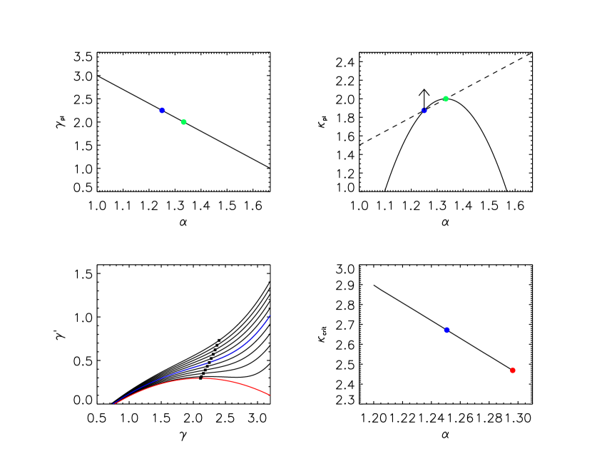
Figure 1.— Top panels: the $\gamma(\alpha)$ and $\kappa(\alpha)$ relations for the powerlaw solutions of the Jeans equation, see § 2.1; blue dots refer to the solution with $\alpha=5/4$, and green dots refer to the solution with $\alpha=4/3$ (the isothermal sphere). In the right panel the dashed line represents the relation $\kappa=3\,\alpha/2$, and the arrow indicates how $\kappa$ increase toward the values (given in the bottom right panel) for the $\alpha$-profiles, see § 2.1-2.2 for details. Bottom panels: the $\gamma-\gamma^{\prime}$ and $\kappa_{\mathrm{crit}}(\alpha)$ relations for the $\alpha$-profiles with $\alpha$ in the range $1.2-35/27$, see § 2.1-2.2; blue dots and curves refer to the solution with $\alpha=5/4$, and red dots and curves refer to the solution with $\alpha=35/27$. In the left panel, the squares mark the couple of values $\gamma_{0}$, $\gamma_{0}^{\prime}$ at $r=r_{0}$. Note that we will find in § 3 the relevant values of $\alpha$ to be constrained within the range $5/4-35/27$, i.e., between the blue and red dots/curves.

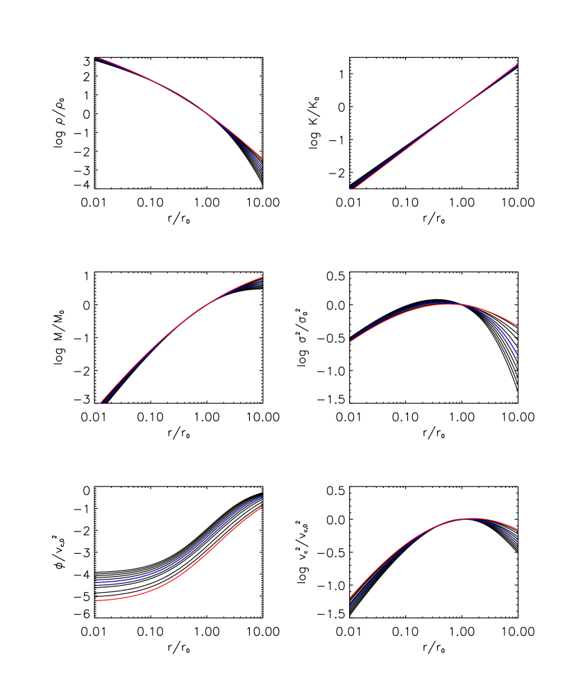
Figure 2.— Radial runs for the $\alpha$-profiles: density $\rho$, mass $M$, circular velocity $v_{c}$, gravitational potential $\Phi$, velocity dispersion $\sigma$, and entropy $K$; the profiles are normalized to $1$ at the point $r_{0}$ where $\gamma=\gamma_{0}=6-3\,\alpha$ holds. Various curves are for $\alpha$ in the range $1.2-35/27$; the blue one refers to the solution with $\alpha=5/4$, and the red one refers to $\alpha=35/27$.

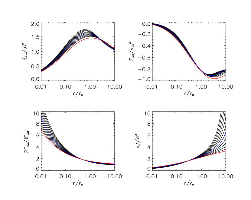
Figure 3.— Energy distributions for the $\alpha$-profiles: specific potential energy $E_{\mathrm{pot}}$, random kinetic energy $E_{\mathrm{kin}}$, virial ratio $2\,E_{\mathrm{kin}}/|E_{\mathrm{pot}}|$, and ratio of circular velocity to the velocity dispersion $v_{c}^{2}/\sigma^{2}$ appearing in Eq. (2). Lines as in Fig. 2.

2. Jeans equilibria

The static equilibria of the DM halos obey the Jeans equation that, on neglecting for the time being anisotropies and the blend into the large-scale environment to be discussed in § 5, reads

$${1\over\rho}{\mathrm{d}(\rho\,\sigma^{2})\over\mathrm{d}r}=-\,{GM(<r)\over r^{2}}~{}.$$ (1)

To elicit the contents of this macroscopic-like equation, an explicit link is required between $\sigma^{2}(r)$ and $\rho(r)$. Such a link may be provided by $Q(r)$, or by the equivalent quantity $K(r)\equiv\sigma^{2}/\rho^{2/3}=Q^{-2/3}(r)$; this is often named DM ‘entropy’ in view of its formal analogy with the adiabat of a gas in thermal equilibrium, and is increasingly used in the context of DM equilibria, from Taylor & Navarro (2001) to Faltenbacher et al. (2007). We focus on this function of state $K(r)$ in the configuration space, and comment on our choice in § 5.

In terms of the slope $\mathrm{d}\log K/\mathrm{d}\log r\equiv\alpha$, Eq. (1) is recast into the particularly simple form

$${5\over 3}\,{\mathrm{d}\log\,\rho\over\mathrm{d}\log\,r}=-{\mathrm{d}\log\,K\over\mathrm{d}\log\,r}-{v^{2}_{c}(r)\over\sigma^{2}(r)}~{}.$$ (2)

Here $v_{c}^{2}(r)=G\,M(<r)/r$ is the (squared) circular velocity, that provides a natural scaling for the depth of the DM potential well.

Taking up from the simulation phenomenology only the notion that $\alpha$ be uniform throughout the halo bulk (see § 1), we will discuss the range of values to be expected for $\alpha$ as a clue to their origin. In fact, in their pioneering work Taylor & Navarro (2001) selected a value of the exponent close to $\alpha=1.25$. Other, recent studies have provided similar values for $\alpha$: around $1.27$ according to Ascasibar et al. (2004), and around $1.29$ according to Rasia et al. (2004). Beyond the minor differences, it is the narrow empirical range that constituted an unsolved challenge.

2.1. Background

We begin with looking first (after Taylor & Navarro 2001) at powerlaw solutions of Eq. (2) of the form $\rho\propto r^{-\gamma}$, with the entropy run set to $K\propto r^{\alpha}$; then not only $\alpha$ is a given parameter, but also the slope $\gamma=-\mathrm{d}\log\rho/\mathrm{d}\log r$ is a constant to be determined from Eq. (2) in the form

$$\gamma-{3\over 5}\,\alpha={3\over 5}\,{\kappa\over 3-\gamma}\,\left({r\over r_{0}}\right)^{2-\alpha-\gamma/3}~{}.$$ (3)

Here the ‘bare’ constant $\kappa\equiv 4\pi\,G\rho_{0}\,r_{0}^{2}/\sigma_{0}^{2}=(3-\gamma)\,v_{0}^{2}/\sigma_{0}^{2}$ compares the gravitational potential to the random kinetic energy associated with the velocity dispersion at a reference point $r_{0}$. At the r.h.s. $\kappa$ appears as modulated by $r-$dependencies, produced by the integrated dynamical mass $M(<r)$ to yield $v^{2}_{c}(r)\propto r^{2-\gamma}/(3-\gamma)$ in the powerlaw case, and by the local dependencies from $\sigma^{2}(r)\propto K(r)\,\rho^{2/3}(r)\propto r^{\alpha-2\gamma/3}$.

For a powerlaw solution to actually hold the r.h.s. must be constant, which yields the link

$$\gamma=6-3\,\alpha~{},$$ (4)

as pointed out by Taylor & Navarro (2001), Hansen (2004), and Austin et al. (2005). Given this, the balance of the three terms in Eq. (3) imposes on the dimensionless gravitational pull the constraint

$$\kappa=(5\gamma/3-\alpha)(3-\gamma)=6\,(\alpha-1)\,(5-3\,\alpha)~{},$$ (5)

whose nonlinearities reflect the DM self-gravity. Thus the allowed powerlaw solutions must lie on a parabola in the plane $\alpha-\kappa$ and on a straight line in the plane $\alpha-\gamma$, as illustrated in the top panels of Fig. 1; note that to ensure $\kappa>0$ the overall bounds $1<\alpha<5/3$ must hold, implying that $1<\gamma<3$ applies for the powerlaw solutions.

Two notable instances correspond to the values $\alpha=4/3$ and $5/4$. The former yields the standard, singular isothermal sphere with $\gamma=2$ and $\kappa=2$; the latter holds for the value of $\alpha$ originally selected by Taylor & Navarro (2001), and implies $\gamma=9/4$ and $\kappa=15/8$. Note that they are located on the intersections of the parabola Eq. (5) with the line $\kappa=3\,\alpha/2$, see Fig. 1.

The powerlaw solutions of the Jeans equation with slope $\gamma_{0}\equiv 6-3\,\alpha$ will turn out to be tangent to the full solutions at $r=r_{0}$ so as to provide a useful reference slope in the middle of the halo. However, they do not qualify as relevant solutions since at both extremes they suffer of unphysical features: since $1<\gamma<3$ holds as shown above, the force $G\,M(<r)/r^{2}\propto r^{1-\gamma}$ would diverge at the center, while the mass $M(<r)\propto r^{3-\gamma}$ would diverge toward large $r$.

To avoid these drawbacks, in all physically relevant solutions the running slope $\gamma(r)$ is to bend down from the middle value in going toward large and small $r$. In fact, for $r\ll r_{0}$ one can infer from Eq. (3) that asymptotically $\gamma\rightarrow\gamma_{a}\equiv 3\,\alpha/5$ is to hold if the gravitational force is to be finite, which implies that both sides of Eq. (3) vanish (see Austin et al. 2005); on the other hand, for $r\gg r_{0}$ it is seen that either $\gamma\rightarrow\gamma_{b}\equiv 3\,(1+\alpha)/2$ holds or a density cutoff occurs, if the mass $M(<r)$ is to saturate to a constant, implying $v^{2}_{c}(r)\propto 1/r$. In other words, powerlaws with inner $\gamma_{a}$ and outer slope $\gamma_{b}$ will constitute asymptotic or effective approximations to the full solutions. For example, for the value $\alpha=5/4$ one recovers the slopes $\gamma_{a}=3/4$ and $\gamma_{b}=27/8$, found by Taylor & Navarro (2001) in their archetypical full solution.

Thus all full solutions may be conveniently visualized as bent down from the corresponding tangent powerlaw so as to meet the above asymptotic forms at both small and large radii. These solutions will be analytically studied and constrained next. In fact, the solution space of the Jeans equation is analytically rich, so we refer the interested reader to the works by Austin et al. (2005), Dehnen & McLaughlin (2005), and Barnes et al. (2006, 2007) for extensive coverage. Here we summarize the main results and proceed to focus on the ‘critical’ solutions in the terminology of Taylor & Navarro (2001).

To highlight the properties of these solutions with running $\gamma(r)$, it is convenient (see Dehnen & McLaughlin 2005; Austin et al. 2005; also Barnes et al. 2006, 2007) to replace the original Jeans equation $\gamma-3\,\alpha/5=3\,v_{c}^{2}/5\,\sigma^{2}$ with its first and second derivative, and use the differential mass definition $\mathrm{d}M/\mathrm{d}r=4\pi\rho\,r^{2}$, to obtain

$$\gamma^{\prime}-{2\over 3}\,(\gamma-\gamma_{a})\,(\gamma-\gamma_{b})={3\over 5}\,\kappa\,\left({r\over r_{0}}\right)^{2-\alpha}\,\left({\rho\over\rho_{0}}\right)^{1/3}~{},$$

(6)

$$\gamma^{\prime\prime}-\gamma^{\prime}\,\left(\gamma-{2\gamma_{a}+2\,\gamma_{b}-\gamma_{0}\over 3}\right)={2\over 9}\,(\gamma-\gamma_{a})\,(\gamma-\gamma_{0})\,(\gamma-\gamma_{b})~{}.$$

Here $\gamma^{\prime}$ and $\gamma^{\prime\prime}$ denote the first and second logarithmic derivative of $\gamma$ with respect to $r$; in addition, $r_{0}$ is the point where the density slope matches $\gamma_{0}\equiv 6-3\,\alpha$ (see Eq. [4]), while $\gamma_{a}\equiv 3\,\alpha/5$ and $\gamma_{b}\equiv 3\,(1+\alpha)/2$ are shorthands for the inner and the outer effective slopes anticipated above.

In the second equation the normalization constant $\kappa\equiv 4\pi G\rho_{0}r_{0}^{2}/\sigma_{0}^{2}$ does not appear explicitly; however, from the first Eq. (6) evaluated at $r_{0}$ it is easily recognized that

$$\kappa=6\,(\alpha-1)\,(5-3\,\alpha)+5\,\gamma^{\prime}_{0}/3$$ (7)

is related to $\gamma^{\prime}_{0}$, and in a full solution specifically measures the upward deviation of $\kappa$ from the corresponding powerlaw, that is, above the parabola expressed by Eq. (5), see also Fig. 1.

In fact, as the value of $\kappa$ increases at given $\alpha$, the solutions will be progressively curved down both inward and outward of $r_{0}$, to constitute a bundle tangent to the related powerlaw with slope given by Eq. (4). But, as stressed by Taylor & Navarro (2001), only a definite maximal value $\kappa_{\mathrm{crit}}$ can be withstood by the halo at equilibrium, lest the solution develops pathologies like a central hole; this value marks a ‘critical’ solution. Correspondingly, the values for $\kappa_{\mathrm{crit}}(\alpha)$ may be found by a painstaking trial-and-error procedure, as done by Taylor & Navarro (2001) for the particular case $\alpha=5/4$. More conveniently, they may be computed directly through Eqs. (6) and (7); the former also provides the following exhaustive description of the solutions.

In the inner region only three situations possibly arise (Williams et al. 2004, Dehnen & McLaughlin 2005): (i) $\gamma$ attains the value $\gamma_{0}$ asymptotically for $r\ll r_{0}$, which is unphysical since such a solution would end there with a diverging gravitational force; (ii) the solution attains the value $\gamma_{a}$ at a finite radius, and then continues to flatten down to the point of developing a central hole, which is obviously to be avoided; (iii) $\gamma$ approaches the value $\gamma_{a}$ asymptotically for $r\ll r_{0}$, that is the only viable possibility. Thus physical solutions must approach the inner slope $\gamma_{a}$, and must steepen monotonically outwards.

However, not all of them are tenable in view of their outer behavior (Austin et al. 2005, Dehnen & McLaughlin 2005). Here, again three situations formally arise that depend on the value of $\alpha$: (i) $\gamma$ approaches the value $\gamma_{0}$ asymptotically for $r\gg r_{0}$, which occurs for $\alpha>35/27$ and is unphysical since with such a solution the mass would diverge (in practice, it would be ill-defined, see § 5); (ii) $\gamma$ attains the slope $\gamma_{b}$ at a finite radius and then goes to an outer cutoff, that occurs for $\alpha<35/27$ and is physically viable since the cutoffs actually set in at large radii exterior to the halo’s bulk, as discussed below; (iii) $\gamma$ approaches the slope $\gamma_{b}$ asymptotically for $r\rightarrow\infty$ as it occurs for $\alpha=35/27$, which also provides a physically viable solution.

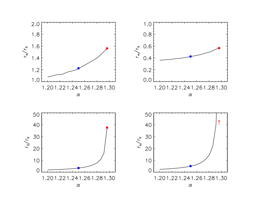
Figure 4.— Characteristic radii (in units of $r_{0}$) for the $\alpha$-profiles as a function of $\alpha$: radius $r_{p}$ where the circular velocity peaks, radius $r_{m}$ where the velocity dispersion peaks, radius $r_{3}$ where the slope of the density profile equals $3$, and radius $r_{b}$ where the slope of the density profile reads $\gamma_{b}=3\,(1+\alpha)/2$. The blue dots refer to the solution with $\alpha=5/4$, and the red dots to $\alpha=35/27$. In the bottom right panel the red arrow indicates that the solution with $\alpha=35/27$ attains the slope $\gamma_{b}$ only asymptotically in a powerlaw tail. Note that as $\alpha$ increases, the peak of the velocity dispersion displaces relatively more than the circular velocity’s.

2.2. Viable full solutions

Summing up, the critical solutions satisfy both sets of criteria, but exist only for $\alpha\leq 35/27=1.\overline{296}$ (which excludes the case corresponding to the isothermal powerlaw); hereafter these will be named ‘$\alpha$-profiles’. We compute them by integrating the second of Eqs. (6) with boundary conditions $\gamma\rightarrow\gamma_{a}$ and $\gamma^{\prime}\rightarrow 0$ for $r\rightarrow 0$. The results in the plane $\gamma-\gamma^{\prime}$ for various $\alpha$ between $1.2$ and $35/27$ are plotted as different lines in Fig. 1 (left bottom panel); there we can read out the values of $\gamma^{\prime}_{0}$ at $r=r_{0}$ (squares in the figure), and find the related $\kappa_{\mathrm{crit}}$ after Eq. (7). The relation $\kappa_{\mathrm{crit}}(\alpha)$ is plotted in Fig. 1 (right bottom panel); the resulting correlation is fitted by the expression $\kappa_{\mathrm{crit}}(\alpha)\simeq 8.228-4.443\,\alpha$ to better than $1\%$.

Our solutions include the prototypical one corresponding to $\alpha=5/4$ (highlighted in blue), first found by Taylor & Navarro (2001) and shown to be well fitted, if only in a region around $r_{0}$, by the NFW formula (Navarro et al. 1997); for such a solution the precise value of $\kappa_{\mathrm{crit}}$ reads $2.674$, see Dehnen & McLaughlin (2005). Our solutions also include the one corresponding to the limiting value $\alpha=35/27$ (highlighted in red) studied by Dehnen & McLaughlin (2005); for this $\kappa_{\mathrm{crit}}=200/81$ is found.

In Fig. 2 we illustrate the radial dependencies of various interesting quantities for the $\alpha$-profiles: density $\rho$ and its logarithmic slope $\gamma$, circular velocity $v^{2}_{c}$, velocity dispersion $\sigma^{2}$, entropy $K$, mass $M(<r)$, and gravitational potential $\Phi=-\int_{r}^{\infty}{\mathrm{d}r^{\prime}}\,G\,M(<r^{\prime})/r^{\prime 2}$; the profiles are normalized to $1$ at the point $r_{0}$ within the halo’s middle. Outwards of this, solutions corresponding to larger values of $\alpha$ have larger overall masses, flatter density profiles, higher velocity dispersions, and deeper potential wells.

As mentioned above, the $\alpha$-profiles with $\alpha<35/27$ show an outer cutoff, to which the following remarks apply. First, the cutoffs generally occur beyond the virial radius (see § 5). Second, the velocity dispersion $\sigma^{2}\propto\rho^{2/3}\,K\propto r^{\alpha-2\gamma/3}$ falls rapidly outside of $r_{0}$ and vanishes at the density cutoff, thus preventing any finite outflow related to residual random motions of DM particles. Third, the microscopic distribution function as obtained through the Eddington formula (e.g., Binney & Tremaine 1987) from pairs of $\rho(r)$ and $\Phi(r)$ is realistic being nowhere negative (see also Zhao 1996; Widrow 2000).

In Fig. 3 we show the ratio $v_{c}^{2}(r)/\sigma^{2}(r)$ entering Eq. (2); we also show the energy distributions associated to the $\alpha$-profiles: the specific potential energy $E_{\mathrm{pot}}=4\pi\int_{0}^{r}{\mathrm{d}r^{\prime}}\,$ $r^{\prime 2}\,\rho(r^{\prime})\,v_{c}^{2}(r^{\prime})/M(<r)$, the random kinetic energy $E_{\mathrm{kin}}=4\pi\int_{0}^{r}{\mathrm{d}r^{\prime}}\,r^{\prime 2}\,\rho(r^{\prime})\;3\,\sigma^{2}(r^{\prime})/2\,M(<r)$, and the local virial ratio $2\,E_{\mathrm{kin}}/|E_{\mathrm{pot}}|$. Note that the latter tends to $1$ at large $r$, as is expected for stable self-gravitating halos (see Łokas & Mamon 2001); in fact, it closely approaches unity already for $r\approx r_{0}$.

In Fig. 4 we plot as a function of $\alpha$ various characteristic radii (in units of $r_{0}$) of the $\alpha$-profiles; specifically, we show the radius $r_{p}$ where the circular velocity $v_{c}(r)$ peaks, the radius $r_{m}$ where the velocity dispersion $\sigma^{2}(r)$ peaks, the radius $r_{3}$ where the slope of the density profile reads $\gamma=3$, and the radius $r_{b}$ where the slope of the profile takes on the value $\gamma_{b}=3\,(1+\alpha)/2$. Note that $r_{b}$ is always large, and formally recedes to infinity (as represented in the plot with an arrow) for the limiting case $\alpha=35/27$ that has a powerlaw falloff.

For the sake of clarity, in these Figures we have confined the values of $\alpha$ to between $1.2$ and $35/27$; although the upper bound is already required for having no central hole and a finite mass as discussed above, limited information existed so far concerning lower bounds from the isotropic Jeans equation.

3. The entropy slopes from
cosmogonic buildup

Here we show that the cosmogonic histories of DM halos enforce additional, stringent limitations to the range of $\alpha$; on the high side the resulting bound turns out to be pleasingly close to the value $35/27$ derived above from the analysis of the static Jeans equation, but on the low side it constitutes a new stringent result.

Consider a DM halo with current bounding radius $R$, density $\rho$, mass $M\propto\rho\,R^{3}$, velocity scales $\sigma^{2}\propto v_{c}^{2}\propto M/R$, and entropy $K\propto\sigma^{2}/\rho^{2/3}$. During the hierarchical buildup the running growth rate scales as $\dot{M}\propto\rho\,v\,R^{2}$ with the inflow speed $v$ set by the depth of the DM well and hence proportional to $v_{c}^{2}$; thus the above quantities may be expressed in terms of $M$ and $\dot{M}$ to provide the scaling laws:

$$R\propto M/\dot{M}^{2/3}~{}~{}~{}~{}~{}~{}v_{c}^{2}\propto\sigma^{2}\propto\dot{M}^{2/3}~{}~{}~{}~{}~{}~{}\rho\propto\dot{M}^{2}/M^{2}~{}~{}~{}~{}~{}~{}K\propto M^{4/3}/\dot{M}^{2/3}~{}.$$ (8)

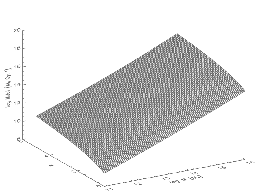
Figure 5.— The relation $\dot{M}(M,z)$ from the average cosmogonic evolution, see § 3.2 for details.

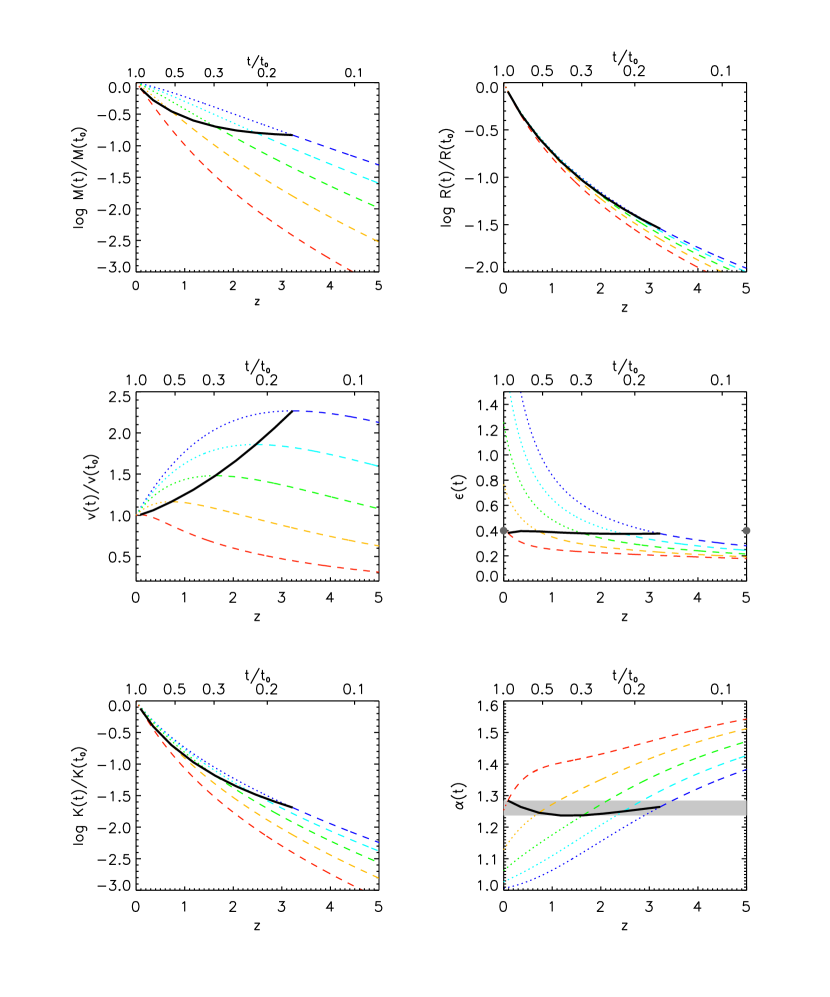
Figure 6.— Evolution of the various quantities along the average accretion history of DM halos: mass $M$, radius $R$, velocity $v$, (inverse) mass growth rate $\epsilon=-\mathrm{d}\log(1+z)/\mathrm{d}\log M$, entropy $K$, and slope $\alpha\equiv\mathrm{d}\log K/\mathrm{d}\log R$. The curves are for different current halo masses in the range $10^{11}-10^{15}\,M_{\odot}$; from top to bottom, blue lines refers to $10^{11}\,M_{\odot}$, cyan to $10^{12}\,M_{\odot}$, green to $10^{13}\,M_{\odot}$, orange to $10^{14}\,M_{\odot}$, and red to $10^{15}\,M_{\odot}$. Lines are dashed in the fast accretion regime, and dotted in the slow accretion phase; the solid line marks values at the transition epoch, see § 3.3 for details. In the bottom right panel, the shaded area highlights the narrow range expected for the values of $\alpha$ at the transition.

3.1. A heuristic approach

Primarily we look for a link of the entropy slope $\alpha$ with the mass growth rate in simple terms; this analysis will have only heuristic scope, introductory to the full study performed in § 3.2. Toward our scope, we make contact with the classic line of developments (Fillmore & Goldreich 1984; Lu et al. 2006) that analytically relate the collapse histories to the shape and growth rate of the primordial DM perturbations. The former may be expressed in terms of $\delta M/M\propto M^{-\epsilon}$; but since a halo virializes when $\delta M/M$ attains a critical threshold (e.g., $1.686$ in the critical universe), the shape parameter $\epsilon=-\mathrm{d}\log(1+z)/\mathrm{d}\log M$ effectively governs also the (inverse) mass growth rate defined in terms of the scaling $M\propto(1+z)^{-1/\epsilon}$.

Then we use the standard relations between redshift $z$ and cosmic time $t$, that may be expressed in the form $(1+z)\propto t^{-q}$. In the critical cosmology $q=2/3$ holds; in the canonical Concordance Cosmology the value $q\approx 2/3$ still applies to $z\gtrsim 1$, but as $z$ decreases $q$ progressively rises to values $q\approx 0.8$ for $z\lesssim 0.5$. Then the mass growth history writes simply $M\propto t^{q/\epsilon}$ and the growth rate reads $\dot{M}/M=q/\epsilon\,t$; from Eqs. (8), simple algebra yields the scaling laws $R\propto t^{(2+q/\epsilon)/3}$, $\rho\propto t^{-2}$, and $K\propto t^{2\,(1+q/\epsilon)/3}$. On eliminating $t$ one obtains $K\propto R^{\alpha}$ and $\rho\propto R^{-\gamma}$ with slopes

$$\alpha=1+{1\over 1+2\,\epsilon/q}~{}~{}~{}~{}~{}\mathrm{and}~{}~{}~{}~{}~{}~{}\gamma={6\,\epsilon\over 2\,\epsilon+q}~{},$$ (9)

the latter being related to the former by the simple scaling link $\gamma=6-3\,\alpha$, as expected at $r\approx r_{0}$ from Eq. (4). From Eq. (9) $\alpha$ is seen to be slightly larger than unity by a quantity slowly depending on $\epsilon/q$; this is consistent with $K\propto R\,M^{1/3}\propto R^{2-\gamma/3}$, the straightforward message from Eqs. (8) with $M\propto R^{3-\gamma}$.

These relationships for $\alpha$ and $\gamma$ embody in a simple form some relevant cosmogonic and cosmological information. For $z\gtrsim 1$ where $q\approx 2/3$ applies, one explicitly has $\alpha\approx(2+3\,\epsilon)/(1+3\,\epsilon)$ and relatedly $\gamma\approx 9\,\epsilon/(1+3\,\epsilon)$, the latter being the well-known expression for the similarity solutions to the spherical infall model in a critical Universe. For $z\lesssim 0.5$ instead when $q\approx 4/5$ applies, one has $\alpha=(4+5\,\epsilon)/(2+5\,\epsilon)$ and $\gamma\approx 15\,\epsilon/(2+5\,\epsilon)$. As said, the remaining parameter $\epsilon$ governs both the shape of the initial perturbations and the times of their collapse. For instance, if the standard top-hat shape applied with $\epsilon\approx 1$ corresponding to a monolithic collapse, from the above relations one would obtain $\alpha\approx 1.25$ and $\gamma\approx 2.25$ for halos that virialize at $z\gtrsim 1$, as pointed out early on by Bertschinger (1985); for more massive halos that virialize at $z\lesssim 0.5$, from the scaling laws one anticipates a slightly steeper $\alpha\approx 1.29$ and a flatter $\gamma\approx 2.15$.

Qualitatively, different values of the slope $\gamma$ may be related to other values of $\epsilon$, such as occurring in an articulated shape of the initial perturbations, that also yields a sequence of collapse times. With a realistic bell-shaped perturbation $\epsilon\approx 1$ still applies to its middle; in the outer regions $\epsilon\gtrsim 1$ implies the accretion to become slower, and correspondingly the density slope $\gamma$ to steepen there relative to the middle one. The central regions are described by $\epsilon\ll 1$, corresponding to fast collapse; the scaling law then suggests the density slope to be flatter there.

However, this simple approach cannot be carried very far. At small radii also angular momentum effects come into play to lower the density profile; they introduce another radial scaling related to centrifugal barriers, as discussed in detail by Lu et al. (2006); these authors show how a density slope around $-1$ is enforced if efficient isotropization of particles’ orbits takes place during the fast collapse, while still flatter slopes occur with more even angular momentum distributions. These, however, must be consistent with the overall equilibrium requirements; these orbital features are actually subsumed into the macroscopic Jeans Eq. (2) with $K\propto r^{\alpha}$ and provide the running $\gamma(r)=3\,\alpha/5+3\,v_{c}^{2}(r)/5\,\sigma^{2}(r)$ (the last term is shown in Fig. 3) that is to replace the stiff scaling value $\gamma=6-3\,\alpha$ above, but still recovers it at the single radius $r_{0}$ (cf. Eqs. [4] and [6]).

So we will depart from the above heuristic approach, and focus on computing the values of $\alpha$ to be inserted into Jeans, also implementing precise mass and time dependencies of the growth rate $\epsilon$. To focus these sensitive issues a refined analysis and a careful discussion are required and performed next.

3.2. Advanced, semianalytic analysis

We derive a robust time evolution and mass dependence of $\dot{M}$ from an updated version of the Extended Press & Schechter formalism (EPS, see Lacey & Cole 1993).

We are mainly interested in the average evolutionary behavior of halos, so we compute the mean growth rate $\dot{M}$ of the current mass $M$ as

$$\dot{M}=\int_{0}^{M}{dM^{\prime}}~{}(M-M^{\prime})\,{\mathrm{d}^{2}P_{M^{\prime}\rightarrow M}\over\mathrm{d}M^{\prime}\mathrm{d}t}~{},$$ (10)

in terms of the differential merger rate $\mathrm{d}^{2}P_{M^{\prime}\rightarrow M}/\mathrm{d}M^{\prime}\mathrm{d}t$ given in Appendix A. This incorporates the full cosmological framework, and the detailed cold DM perturbation spectrum; as to the former we implement the Concordance Cosmology, and as for the latter we adopt the shape given by Bardeen et al. (1986) corrected for baryons (Sugiyama 1995), and normalized as to yield a mass variance $\sigma_{8}=0.8$ on a scale of $8\,h^{-1}$ Mpc. We improve over previous studies of this kind (e.g., Miller et al. 2006; Li et al. 2007; Salvador-Solé et al. 2007) by using the merger rate appropriate for ellipsoidal collapses (Sheth & Tormen 2002) as provided by Zhang et al. (2008); this is shown by the latter authors to yield formation times and growth rates in much closer agreement with numerical simulations than the standard EPS theory. Further details are presented in Appendix A.

Eq. (10) provides the relation $\dot{M}(M,t)$ illustrated in Fig. 5. This may be viewed as a first order differential equation for $M(t)$, that is numerically solved once the mass $M(t_{0})$ at the present time $t_{0}$ has been assigned in the way of a boundary condition. In terms of $M(t)$ so computed, the evolution of the halo properties are obtained through Eqs. (8); the results are illustrated in Fig. 6, where we plot the time and redshift evolutions for the inverse growth rate $\epsilon$, the overall radius $R$, the mass $M$, the characteristic velocities $v\propto\sigma$, the entropy $K$, and finally the corresponding slope $\alpha\equiv\mathrm{d}\log K/\mathrm{d}\log R$. The curves are for different current values of the halo masses $M(t_{0})$ ranging from $10^{11}$ to $10^{15}\,M_{\odot}$.

In fact, in these detailed mass accretion histories one can recognize a transition epoch when the circular velocity $v_{c}^{2}$ of the halo attains its highest value along an accretion history (see Li et al. 2007). The transition separates two stages: an early stage of fast collapse, when $\epsilon\lesssim 0.4$ corresponds to a growth rate still high on the running Hubble timescale, and nearly constant; and a later phase of slower accretion when $\epsilon$ takes off from the value $0.4$, i.e., the growth rate is low and decreasing. Small halos with $M\lesssim 10^{12}\,M_{\odot}$ have high transition redshifts, hence are now well advanced into their slow accretion stage; on the other hand, very massive ones with $M\gtrsim 10^{15}\,M_{\odot}$ have low transition redshifts, so today they have just completed their fast accretion stage. A similar behavior has been identified in a number of recent numerical simulations (Zhao et al. 2003; Diemand et al. 2007), and has been recognized also in other semianalytic computations based on the simpler, less precise EPS theory (see Li et al. 2007; Neistein et al. 2006).

3.3. Results

From Fig. 6 we also see that the values of $\alpha$ at the transition are narrowly constrained to within $1.27\pm 0.02$, i.e., a $1.5\%$ range. We note that this range explains why narrowly constrained phenomenological values of $\alpha$ are found within the halo bulk from many and different simulations since the year 2000. In particular, our values turn out to agree with the best fitting exponent of $Q(r)$ [or $K(r)$] with its scatter recently given in detail by Ascasibar & Gottlöber (2008) within the halo bulk during calm infall; these authors warn against extrapolating their results to early times and outer radii.

Correspondingly, in our findings the values of $\alpha$ before the transition should not be overinterpreted nor inserted into the Jeans equation. In fact, at these early epochs the halos experience rapid changes and are clearly out of equilibrium; during this stage the $N-$body experiments (see Zhao et al. 2003; Peirani et al. 2006; Hoffman et al. 2007) highlight turmoil associated with fast collapse and major mergers, effective dynamical relaxation and mixing of DM particles. Taking up from § 3.1, it is during these events that the orbits’ angular momentum must set to a near isotropic distribution such as to lower the inner densities.

But as the turmoil associated with the fast collapse subsides, the orbital structure is bypassed and replaced by the macroscopic entropy distribution $K\propto r^{\alpha}$ with uniform values of $\alpha$, as phenomenologically found to hold throughout the now stable halos’ bulk. Then the values of $\alpha$ at the transition epoch and the corresponding edge $R=r_{0}$ can be derived from the scaling laws and applied to the whole inner region, to obtain $\gamma(r)=3\,\alpha/5+3\,v_{c}^{2}(r)/5\,\sigma^{2}(r)$, taking on the value $6-3\,\alpha$ only at the point $r_{0}$ according to the results of § 2.1.

The value of $\alpha$ is expected to persist in the bulk during the subsequent development in the slow accretion stage, when mass is added smoothly and mainly onto the outskirts, with little mixing. Such a development is borne out by the widely shared scenario of halo buildup from the inside out, championed by Bertschinger (1985), Taylor & Navarro (2001), and many others up to Salvador-Solé et al. (2007). Specifically, the analysis by the former authors concerning the randomization and the stratification of particles’ orbits during secondary infall indicates that their internal disposition is little affected by subsequent, smoother mass additions on top of a closely static potential well. Thus during the late, slow accretion stage the structure for $r\lesssim r_{0}$ will be unaffected.

Meanwhile, the outer scale $R\propto M/\dot{M}^{2/3}$ beyond $r_{0}$ is increasingly stretched out to substantially larger values (see Fig. 6, top right panel); correspondingly, we find the outer slope $\alpha(R)\equiv\mathrm{d}\log K/\mathrm{d}\log R$ at $R>r_{0}$ to decline in time (see Fig. 6, bottom right panel). This translates into a radial decrease $\alpha(r)$ on maintaining entropy stratification also into these regions (see Bertschinger 1985, Taylor & Navarro 2001). Such a decrease is to be expected also from considering that $K(r)\propto r^{2-\gamma/3}\rightarrow r$ applies, on the basis of the related asymptotic behaviors of $\rho(r)\propto r^{-\gamma}$ and $\sigma^{2}(r)\propto r^{2-\gamma}$ where $\gamma\rightarrow 3$. We find the values of $\alpha$ to decrease by less than $2\%$ out to $r\approx 2\,r_{0}$, and less than $10\%$ out to $r\approx 5\,r_{0}$.

Concerning the Jeans equation, this too (with its boundary conditions set at $r=0$, see § 2.2) technically works from the inside out, and may be extended to the range $r>r_{0}$ with decreasing slope $\alpha(r)$. The corresponding density run is somewhat steepened for $r>r_{0}$, as if shifting from the upper to the lower curves in Fig. 2; we have checked that the outer density profile lowers by less than $20\%$ for $r\lesssim 5\,r_{0}$. State-of-the-art simulations still yield little information on the outskirts for $r\gtrsim r_{0}$ owing to low densities and noisy data there discussed by Ascasibar & Gottlöber (2008). We present elsewhere the complete solutions outside $r_{0}$ as a testbed for future simulations aimed at resolving the outskirts, and at fitting gravitational lensing observations (see discussion in § 5).

In a similar vein, we predict a minor increase of $\alpha$ at the transition from $1.25$ to $1.29$ in moving from galaxy- to cluster-sized current masses. A fit accurate to better than $0.1\%$ to this average relation is provided by $\alpha\simeq 2.71-0.23\,\log(M/M_{\odot})+0.009\,[\log(M/M_{\odot})]^{2}$; in particular for galaxy clusters, this implies values of $\alpha\approx 1.27$ for Abell richness classes $\mathfrak{r}\approx 0$ and $\alpha\approx 1.29$ for richness class $\mathfrak{r}\gtrsim 3$. The correlation $\alpha(M)$ may help to understand the differences in the values of $\alpha$ found in numerical simulations; in fact, the highest value $1.29$ to date has been reported by Rasia et al. (2004) in looking at cluster-sized halos, while the value $1.25$ first found by Taylor & Navarro (2001) refers to galaxy-sized halos. Observational evidence supporting the above picture is presented in § 5.

To sum up, from the cosmological buildup we find for the entropy slope the narrow allowed range

$$\alpha\approx 1.27\pm 0.02~{};$$ (11)

this we use in our Jeans-like description of DM equilibria within the halos’ bulk. The bounds on $\alpha$ are relevant in two respects: the upper one strengthens the formal limit $35/27=1.\overline{296}$ required for the solutions of the static Jeans equation to have viable profiles in the far outskirts (see § 2.2 and discussion in § 5); the lower one complementarily restricts the range of the viable values.

4. A physical meaning for $\kappa_{\mathrm{crit}}$

Here we propose to discuss the physical meaning of the quantity $\kappa_{\mathrm{crit}}$ (defined in § 2.1 following Taylor & Navarro 2001) in terms of a direct energetic argument. We first note that given the asymptotics of the $\alpha$-profiles, the velocity dispersion $v_{c}^{2}(r)$ must peak at a point $r_{p}\gtrsim r_{0}$ (see Fig. 4) to the value $v_{p}^{2}=4\pi G\rho(r_{p})\,r_{p}^{2}$; at this easily identified point the constant $\kappa$ also writes $4\pi G\rho(r_{p})\,r_{p}^{2}/\sigma_{p}^{2}=v_{p}^{2}/\sigma_{p}^{2}$, and thus is seen to compare the estimate $\sigma_{p}^{2}$ for the random kinetic energy with the estimate $v^{2}_{p}$ for the gravitational potential. We then recall from § 2.1 that a halo in the viable equilibrium condition for a given $\alpha$ is marked by a maximal value $\kappa_{\mathrm{crit}}(\alpha)$, that is, by a minimal level of randomized energy $\sigma^{2}_{p}=v_{p}^{2}/\kappa_{\mathrm{crit}}$.

We now show that to a very good approximation the value for $\kappa_{\mathrm{crit}}$ may be obtained from considering incomplete conversion of the infall kinetic energy $v_{\mathrm{inf}}^{2}/2$ of DM particles into their dynamically randomized energy $3\,\sigma^{2}_{p}/2$ during formation; a process introduced by Bertschinger (1985), different from the complete violent relaxation proposed by Lynden-Bell (1967) and discussed widely, including the recent Arad & Lynden-Bell (2005), Trenti & Bertin (2005) and Trenti et al. (2005).

We propose to derive the critical value of $\kappa=v_{p}^{2}/\sigma_{p}^{2}$ from the relation

$$3\,\sigma_{p}^{2}\approx\eta\,v_{\mathrm{inf}}^{2}~{},~{}~{}~{}~{}~{}\mathrm{with}~{}~{}~{}~{}~{}\eta={3\over 2}\,{v_{p}^{2}/v_{\mathrm{inf}}^{2}\over 1+v_{p}^{2}/v_{\mathrm{inf}}^{2}}~{}.$$ (12)

This expression for the effective conversion efficiency $\eta$ has been constructed on considering that: (i) it has to depend on the ratio of the ($1-$D) infall velocity squared $v_{\mathrm{inf}}^{2}$ to the depth of the potential well as measured by the ($2-$D) circular velocity squared $v_{p}^{2}$; (ii) the formal limit $v_{p}^{2}=2\,\sigma_{p}^{2}$ corresponding to $\kappa=2$ (the isothermal powerlaw, see § 2.1) must be approached for a fast inflow with $v_{\mathrm{inf}}^{2}\gg v_{p}^{2}$, which quantifies the incompleteness of the energy conversion during the transit of a bullet with crossing time short compared with the halo’s dynamical time.

As a simple example guided by the canonical theory of gravitational interactions (see Saslaw 1985; Cavaliere et al. 1992) we may consider that $v_{\mathrm{inf}}^{2}/v_{p}^{2}\approx 3$ is to hold for having considerable energy transfer; using this simple approximation in Eq. (12) yields $\kappa_{\mathrm{crit}}\approx 2.\overline{6}$, a value pleasingly close to $2.64$ as obtained numerically in § 2.2 for the particular $\alpha$-profile with $\alpha=1.25$. On the other hand, this simple argument cannot pinpoint values of $\kappa_{\mathrm{crit}}$ to the precision required to discriminate different values of $\alpha$.

So, we may test our proposed $\eta$ as given in Eq. (12) for different values of $\alpha$ by using instead energy conservation to express the infall velocity $v_{\mathrm{inf}}^{2}\approx 2\,\Delta\phi_{pt}$ in terms of the adimensional potential drop $\Delta\phi_{pt}$ (normalized to $v_{p}^{2}$) from the turnaround radius to $r_{p}$ (see Bertschinger 1985; Lapi et al. 2005). Inserting this into Eq. (12) yields the expression

$$\kappa_{\mathrm{crit}}\equiv{v_{p}^{2}\over\sigma_{p}^{2}}=2+{1\over\Delta\phi_{pt}}~{};$$ (13)

this highlights the deviation of $\kappa_{\mathrm{crit}}$ from the value $2$ that would apply for the isothermal powerlaw (see § 3). Using the runs of $\phi$ appropriate for the $\alpha$-profile as given in Fig. 2, we compute values for $\kappa_{\mathrm{crit}}$ as a function of $\alpha$; note that these decrease for increasing $\alpha$ which implies larger $\Delta\phi_{pt}$, see Fig. 2. Fig. 7 shows how well Eq. (13) recovers the $\kappa_{\mathrm{crit}}(\alpha)$ relation obtained through numerical integration of the Jeans equation.

This excellent fit to $\kappa_{\mathrm{crit}}$ means that the expression for $\eta$ in Eq. (12), more than a successful guess, is describing what actually occurs in the macroscopic equilibria expressed by the Jeans equation in keeping with the numerical simulations. At the referee’s suggestion we add that what ultimately the first Eq. (12) describes with the isotropic form of its l.h.s. is a partial effective conversion at $r\approx r_{p}$ from radial infall into tangential motions.

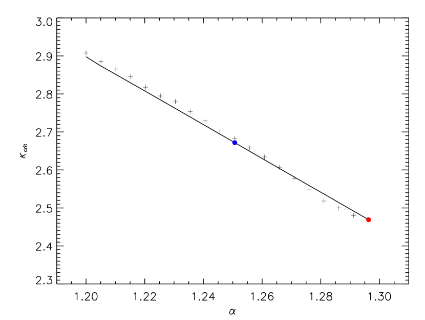
Figure 7.— The $\kappa_{\mathrm{crit}}(\alpha)$ relation, as in Fig. 1 (bottom right panel). Crosses illustrate the goodness of our approximation to $\kappa_{\mathrm{crit}}(\alpha)$ based on a direct energetic argument, see § 4 for details.

Figure 8.— Analytic fits to the density runs (top panels) and residuals (bottom panels) for the $\alpha$-profiles with $\alpha=1.25$ (left panels) and $\alpha=35/27$ (right panels). Solid lines illustrates the exact solutions from numerical integration of the Jeans equation, dashed lines show our analytic fitting formula Eq. (B1), and dotted line (only in left panels) is the fitting formula by Taylor & Navarro (2001, their Eq. [10]); note that Eq. (B1) for $\alpha=35/27$ coincides with the exact solution given by Dehnen & McLaughlin (2005).

5. Discussion and conclusions

The general picture of DM halo formation as it emerges from recent $N-$body simulations envisages a progressive buildup through a two-stage development. At early epochs major mergers associated with fast reshaping of the bulk gravitational potential cause particles’ orbits to dynamically relax and mix into a definite equilibrium disposition. At later epochs the halo outskirts progressively build up through rare if persisting minor mergers and by smooth mass accretion, settling to a quasi-static equilibrium.

The stable equilibria soon after the early stage are effectively described in terms of a phenomenological entropy run $K\propto r^{\alpha}$ with uniform slope $\alpha$ somewhat larger than $1$. Spurred by this powerlaw behavior, one might look for powerlaw solutions of the Jeans equation for the equilibrium density profiles, only to find these just tangent to the actual solutions. From here our analysis goes beyond powerlaw densities, and provides two related blocks of novel results.

First, we have computed and illustrated a wide set of novel solutions to the isotropic Jeans equation, that we name $\alpha$-profiles, including as two particular instances the prototypes investigated by Taylor & Navarro (2001) and Dehnen & McLaughlin (2005). We have stressed that at given $\alpha$ the solutions form a tangent bundle with $\rho(r)$ progressively curved down as the gravitational pull measured by $\kappa=v_{p}^{2}/\sigma_{p}^{2}$ increases above the value corresponding to the pure powerlaw profile $\gamma=6-3\,\alpha$; from such bundles the $\alpha$-profiles stand out for having a shape maximally curved to the point of complying with sensible outer and inner behaviors, i.e., finite total mass and no central hole. This occurs for a maximal value $\kappa_{\mathrm{crit}}(\alpha)$ of the gravitational pull $v_{p}^{2}$ relative to the random component $\sigma_{p}^{2}$, i.e., for a minimal $\sigma_{p}^{2}$ compared to $v_{p}^{2}$; this also corresponds to the maximal slope $\gamma_{p}=3\,\alpha/5+\kappa_{\rm crit}$ at the point $r_{p}$. Such solutions still constitute a large set, being parameterized in terms of a wide overall range $1<\alpha\leq 1.\overline{296}$ for the values of $\alpha$.

Second, we have shown that toward further constraining these values the key step is provided by the halos’ cosmological buildup; in fact, the scaling laws of § 3 narrowly restrict the viable range to $\alpha\approx 1.25-1.29\approx 1.27\pm 0.02$, corresponding to current masses $M\sim 10^{11}-10^{15}\,M_{\odot}$. We have found these bounds to apply at the epochs of transition from fast collapse to slow accretion, when the potential wells settle to their maximal depths along an accretion history (see § 3). In fact, our semianalytic analysis not only recovers the two-stage development observed in many recent $N-$body simulations, but also explains why only such narrowly constrained values of $\alpha$ are actually found in many different numerical works since the year 2000. The values $\kappa_{\mathrm{crit}}$ is correspondingly constrained to the range $2.7\gtrsim\kappa_{\mathrm{crit}}\gtrsim 2.5$; we trace back these values to limited randomization for the infall kinetic energy of DM particles during accretion, which leads to minimal values of $\sigma^{2}$.

The $\alpha-$profiles from the Jeans equilibrium with $\alpha$ and $\kappa_{\mathrm{crit}}$ so constrained imply that galaxies have a generally more compact central structure than groups and clusters, with appreciable deviation from self-similarity; on the other hand, the former have currently developed extensive outskirts, while the very rich clusters do not yet.

To embody in a handy expression the basic features of the density runs for the $\alpha-$profiles, we provide here an analytic fitting formula of the form often advocated on phenomenological grounds (see Zhao 1996; Kravtsov et al. 1998; Widrow 2000; Barnes et al. 2006), that reads

$$\rho(r)\propto{1\over\left({r/r_{0}}\right)^{\gamma_{a}}\,\left[1+w\,\left({r/r_{0}}\right)^{u}\right]^{q}},$$ (14)

with $\gamma_{a}$ governing the inner profile, $q$ the outer one, $w$ and $u$ the position and sharpness of the radial transition. Here for the first time such a profile is substantiated with parameters expressed in terms of the derivatives of the Jeans equation (see § 2.2) and of the values for $\alpha$ as detailed in Appendix B. We stress that the Jeans equlibrium (see Fig. 2) requires that the central slopes are always flatter, and the outer ones always steeper than in the empirical NFW fit. The goodness of the above fitting formula is discussed in Appendix B, and illustrated in Fig. 8.

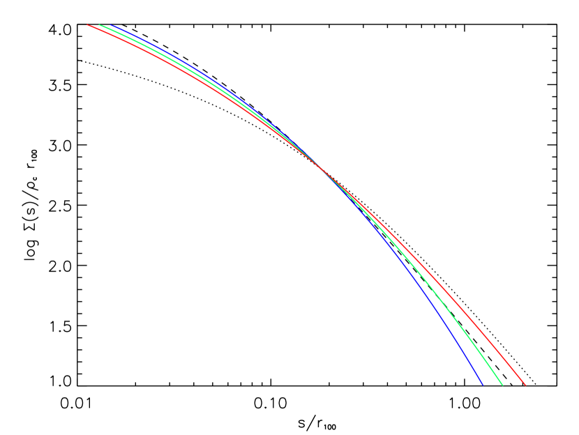
Figure 9.— Surface density runs from the $\alpha$-profiles for $\alpha=1.25$ (blue), $\alpha=1.27$ (green) and $\alpha=1.29$ (red) and from the empirical NFW profile with concentration parameter $c=5$ (black dotted), compared with a fit to the gravitational lensing data by Umetsu & Broadhurst (2008, black dashed) in terms of an NFW profile forced to high concentrations $c\approx 14$, but actually overshooting the central data. Note how our physical profiles do better both in the central and in the outer region while relieving, along with the two-stage development, the problems of high concentrations and short ages that arise from NFW fits as discussed by Broadhurst et al. (2008).

We probe the physical relevance of the $\alpha-$profiles by comparing in Fig. 9 the related projected density runs with the results from recent, exquisite observations of strong and weak gravitational lensing in and around massive galaxy clusters, which just require flat inner, and steep outer behaviors (Broadhurst et al. 2008, Umetsu & Broadhurst 2008, and references therein). It is seen how straightforward are our fits in terms of high-mass $\alpha-$profiles that naturally exhibit just such features, compared to those in terms of the NFW empirical formula that not only has problems of ill-defined mass, but also would require particularly high concentrations and old ages. Our findings substantiate the $\alpha$-profiles, and stress their value as to specific predictions for future simulations aimed at resolving, and for weak gravitational lensing observations aimed at probing the outer cluster densities. A full discussion of these issues deserves a dedicated paper.

Two comments are in order concerning the validity of the Jeans equation in the simple form of Eq. (2). First, reasonable anisotropies in the DM are described by the standard parameter $\beta\equiv 1-\sigma_{\theta}^{2}/\sigma_{r}^{2}$ (Binney 1978), which numerical simulations suggest to increase with $r$ from central values $\beta(0)\approx-0.1\div 0$ meaning near isotropy to outer values close to $0.5$, meaning progressive outward prevalence of radial motions (see Hansen & Moore 2006). Such anisotropies inserted into Jeans produce small variations of the $\alpha-$profiles, to the effect of slightly increasing the limiting value $\alpha=35/27-4\,\beta(0)/27$; thus in the related limiting solutions the inner slope is flattened $\gamma_{a}=3\,\alpha/5+6\,\beta(0)/5=7/9+10\,\beta(0)/9$, the middle slope $\gamma_{0}=6-3\,\alpha=19/9+4\,\beta(0)/9$ is steepened, and the outer slope $\gamma_{b}=3\,(1+\alpha)/2=31/9-2\,\beta(0)/9$ is also steepened with respect to the isotropic case, see Dehnen & McLaughlin (2005). The oppositely extreme case of total radial anisotropy with constant $\beta=\beta(0)\approx 1$ discussed by Austin et al. (2005) would yield a lower limiting $\alpha=31/27\approx 1.148$, while also producing a steep inner slope $\gamma_{a}=17/9\approx 1.88$ (cf. § 2.1). In brief, the distinctive features of the $\alpha-$profiles are somewhat enhanced, if anything, with radially increasing anisotropies.

Second, the static Jeans equation becomes increasingly vulnerable in going into the outermost regions, since static or even dynamic equilibrium is not granted beyond the virial radius. Specifically, in the Concordance Cosmology the Hubble expansion takes over at radii exceeding a few times the virial radius where $\Omega_{\Lambda}\,(H_{0}\,r/v_{c})^{2}\gtrsim 1$ holds. This weakens the case for the formal upper limit $\alpha=35/27$ as derived from Jeans analysis but correspondingly highlights the relevance of the ceiling $\alpha\approx 1.3$ for a few $10^{15}\,M_{\odot}$ halo we have derived from cosmogonic evolution. On the other hand, any halo termination will be uncertain by full factors of $2$; with flat outer density slopes, as the case with $\alpha>35/27$ (see end of § 2.1), the related total masses will be ill-defined by similar factors, corresponding for galaxy clusters to a disturbing uncertainty by $\pm 2$ in Abell richness class (see Yee & López-Cruz 1999).

Finally, we comment on our use of the DM ‘entropy’ $K(r)=\sigma^{2}(r)/\rho^{2/3}(r)$ – actually the analog of the thermodynamic adiabat, related to entropy by $s=3/2\,\log K$ – rather than the equivalent functional ‘phase-space density’ $Q=K^{-3/2}$ – that underlies the ‘information’ $\log Q=-s$ with the obvious minus sign. Matter-of-factly, the pressure gradient $\mathrm{d}\,(\rho\,\sigma^{2})/\mathrm{d}r$ that withstands the self-gravity in Eq. (1) is most directly expressed in terms of the macroscopic quantity $K$, in the form $\mathrm{d}\,(\rho^{5/3}\,K)/\mathrm{d}r$. In the way of interpretations, our lead is provided by the positive-definite gradient $\Delta s=3/2\,\Delta\log K$, and specifically by its adimensional version $\mathrm{d}\log K/\mathrm{d}\log r\equiv\alpha$.

We find $\Delta s$ to be convenient in understanding the empirical evidence as to positive and uniform of $\alpha$ within the halos’ bulk after the transition; then and there, in fact, the particle orbits settle to a definite dynamical regime, relaxed toward a periodic, ordered behavior (Bertschinger 1985), corresponding to lower entropy layers at the center. In the outer regions, on the other hand, the particle orbits stratify but mix poorly during the late, slow buildup (see Bertschinger 1985; Taylor & Navarro 2001) with their apocenters distributed over larger and larger sizes; we understand this dynamical regime in terms of $K$ or $\Delta s$ spread over increasingly stretched radii $R>r_{p}$, resulting in flatter slopes.

It rests with the numerical values of $\alpha$ to translate the fine orbital details into the macroscopic average of Jeans, as clearly indicated by the consistency of the results from the latter with semianalytic cosmogony and with simulations.

We end by stressing that the formulation of DM distribution in terms of ‘entropy’ – despite the standard objections about defining entropy for a collisionless medium out of thermal equilibrium and dominated by long range weak gravity – opens an interesting perspective; this envisages direct comparisons (see Faltenbacher et al. 2007) with the truly thermodynamic entropy of the other major component in galaxy systems, namely, the collisional plasma in local thermal equilibrium constituting the intracluster medium. In fact, in the outer regions these entropies though related as being both originated by conversion of the infall energy under weak gravity, differ owing to their origin from different conversion processes (Lapi et al. 2005; Cavaliere & Lapi 2006); in addition, in the central region of most clusters the hot plasma is heated up by the activity of supermassive black holes originating under strong gravity conditions.

Appendix A A. Merging rate of DM halo under ellipsoidal collapse

To reliably compute the growth rate $\dot{M}$ in Eq. (10), we use the merging rate of DM halos under ellipsoidal collapse as provided by Zhang et al. (2008); this reads

$${\mathrm{d}^{2}P_{M^{\prime}\rightarrow M}\over\mathrm{d}M^{\prime}\mathrm{d}t}={a_{0}\,e^{-a_{1}^{2}\,\Delta\sigma^{2}/2\sigma_{M}^{2}}\over\sqrt{2\pi}\,(\Delta\sigma^{2})^{3/2}}\,\left|{\mathrm{d}\sigma_{M^{\prime}}^{2}\over\mathrm{d}M^{\prime}}\right|\,\left|{\mathrm{d}\delta_{c}\over\mathrm{d}t}\right|\,\left\{1+a_{2}\,\left({\Delta\sigma^{2}\over\sigma_{M}^{2}}\right)^{3/2}\,\left[1+{a_{1}\over\Gamma(3/2)}\,\sqrt{\Delta\sigma^{2}\over\sigma_{M}^{2}}\right]\right\}$$ (A1)

where $\Delta\sigma^{2}=\sigma_{M^{\prime}}^{2}-\sigma_{M}^{2}$ is the difference of the mass variances corresponding to the masses $M^{\prime}$ and $M$, and

$$a_{0}\equiv 0.866\,\left\{1-0.133\,\left[\delta_{c}(z)^{2}/\sigma^{2}_{M}\right]^{-0.615}\right\}~{},$$

$$a_{1}\equiv 0.308\,\left[\delta_{c}(z)^{2}/\sigma_{M}^{2}\right]^{-0.115}~{},$$ (A2)

$$a_{2}\equiv 0.0373\,\left[\delta_{c}(z)^{2}/\sigma^{2}_{M}\right]^{-0.115}~{}.$$

Note that the standard EPS expression for the spherical collapse model (Lacey & Cole 1993; Kitayama & Suto 1996) is recovered on setting $a_{0}=1$ and $a_{1}=a_{2}=0$.

Eqs. (A1) and (A2) involve the critical threshold $\delta_{c}(z)$ for collapse, which is computed according to

$$\delta_{c}(z)=\delta_{c}\,{D(0)\over D(z)}$$ (A3)

in terms of the normalization value $\delta_{c}\approx 1.686\,[1+0.0123\,\log\Omega_{M}(z)]$ and of the growth factor

$$D(z)={5\over 2}\,{\Omega_{M}(z)\over 1+z}\,\left[{1\over 70}+{209\over 140}\,\Omega_{M}(z)-{1\over 140}\,\Omega_{M}^{2}(z)+\Omega_{M}^{4/7}(z)\right]^{-1}~{};$$ (A4)

in the above the quantity $\Omega_{M}(z)=\Omega_{M}\,(1+z)^{3}/[1-\Omega_{M}+\Omega_{M}\,(1+z)^{3}]$ represents the evolved matter density parameter of the Universe in the Concordance Cosmology.

Eqs. (A1) and (A2) also involve the mass variance of the primordial perturbation spectrum, that writes

$$\sigma_{M}^{2}=4\pi\,\int_{0}^{k_{s}}{\mathrm{d}k}\,k^{2}\,P(k)~{},$$ (A5)

where $k_{s}=(6\pi^{2}\bar{\rho}_{M}/M)^{1/3}$ is the wavenumber corresponding to the mass $M$, and $\bar{\rho}_{M}\approx 2.8\times 10^{11}\,\Omega_{M}h^{2}\,M_{\odot}$ Mpc^-3 is the mean background matter density of the Universe. The mass variance is then normalized to the value $\sigma_{8}=0.8$ for the mass corresponding to a scale of $8\,h^{-1}$ Mpc. As for the power spectrum, we adopt the shape

$$P(k)\propto k\,T^{2}(k)$$ (A6)

in terms of the transfer function

$$T(k)\equiv{\log(1+2.34\,q)\over 2.34\,q}\,\left[1+3.89\,q+(16.1\,q)^{2}+(5.46\,q)^{3}+(6.71\,q)^{4}\right]^{-1/4}$$ (A7)

given by Bardeen et al. (1986). Here $q\equiv k/(h\,\Gamma)$ includes the shape correction factor $\Gamma=\Omega_{M}h\,e^{-\Omega_{b}-\sqrt{2h}\,(\Omega_{b}/\Omega_{M})}$ due to baryons, after Sugiyama (1995); we recall that the values $h=0.72$, $\Omega_{M}=0.27$, and $\Omega_{b}=0.044$ are adopted throughout the paper.

Appendix B B. Fitting the density runs of the $\alpha$-profiles

Here we provide an explicit analytic fit to the $\alpha$-profiles, whose numerical computation is sensitive to precise initialization. We use the expression

$$\rho(r)\propto x^{-\gamma_{a}}\,(1+w\,x^{u})^{-q}$$ (B1)

inspired by the exact solution for $\alpha=35/27$ given by Dehnen & McLaughlin (2005), and representing an extension of the NFW (Navarro et al. 1997) formula; in the above $x\equiv r/r_{0}$ is the adimensional radius, the inner slope has been fixed to $\gamma_{a}=3\,\alpha/5$, while $u$, $q$, and $w$ are parameters dependent on $\alpha$ to be determined.

To this purpose, we impose that at $r=r_{0}$ the density slope from Eq. (B1) and its first and second logarithmic derivatives equal those of the $\alpha$-profiles. Thus we find

$$\gamma_{a}+uq\,{\,w\over w+1}=\gamma_{0}~{}~{}~{}~{}~{}~{}~{}~{}~{}~{}~{}~{}{u^{2}\,q\,w\over(1+w)^{2}}=\gamma_{0}^{\prime}~{}~{}~{}~{}~{}~{}~{}~{}~{}~{}~{}~{}{u^{3}\,q\,w\,(1-w)\over(1+w)^{3}}=\gamma_{0}^{\prime\prime}~{}.$$ (B2)

Then we solve the above expressions for $w$, $u$, and $q$, to obtain

$$w=1-{\gamma_{0}^{\prime\prime}\,(\gamma_{0}-\gamma_{a})\over\gamma_{0}^{\prime 2}}~{}~{}~{}~{}~{}~{}~{}~{}q={(\gamma_{0}-\gamma_{a})^{2}\over w\,\gamma_{0}^{\prime}}~{}~{}~{}~{}~{}~{}~{}~{}u={(\gamma_{0}-\gamma_{a})\,(w+1)\over q\,w}~{}.$$ (B3)

The values of $\gamma_{0}^{\prime}$ and $\gamma_{0}^{\prime\prime}$ are easily computed as a function of $\alpha$. First, Eqs. (6) evaluated at $r=r_{0}$ give

$$\gamma_{0}^{\prime}={3\over 5}\,\kappa_{\mathrm{crit}}(\alpha)+{2\over 3}\,(\gamma_{0}-\gamma_{a})\,(\gamma_{0}-\gamma_{b})$$

(B4)

$$\gamma_{0}^{\prime\prime}={2\over 3}\,\gamma_{0}^{\prime}\,(2\gamma_{0}-\gamma_{a}-\gamma_{b})~{};$$

then these quantities are easily recast in terms of $\alpha$ on recalling from the main text (§ 2.2) that $\gamma_{a}=3\,\alpha/5$, $\gamma_{0}=6-3\,\alpha$, $\gamma_{b}=3\,(1+\alpha)/2$, and $\kappa_{\mathrm{crit}}(\alpha)\simeq 8.228-4.443\,\alpha$.

To sum up, Eqs. (B3) and (B4) provide the parameters $w(\alpha)$, $u(\alpha)$, and $q(\alpha)$ as a function of $\alpha$. E.g., for $\alpha=35/27$ we obtain $w=1.00$, $u=0.44$, and $q=6.00$; thus our fitting formula recovers the exact solution by Dehnen & McLaughlin (2005). At the other extreme, for $\alpha=1.25$ we obtain $w=0.23$, $u=0.39$, and $q=20.77$; here our fitting formula approximates well (see Fig. 8) the exact solution, improving upon the fit by Taylor & Navarro (2001, their Eq. [10]). In fact, we find that for any $\alpha$ between $1.25$ and $35/27$ our fit works to better than a few $\%$ throughout the significant radial range from $10^{-1}$ to several $r_{0}$; note that both the radial range and the quality of the fit increase for increasing $\alpha$, up to the point of pinning down the exact solution for $\alpha=35/27$.

References

- (1)
- (2) Arad, I., & Lynden-Bell, D. 2005, MNRAS, 361, 385
- (3)
- (4) Ascasibar, Y. & Gottlöber, S. 2008, ApJ, 386, 2022
- (5)
- (6) Ascasibar, Y., Yepes, G., Gottlöber, S., & Müller, V. 2004, MNRAS, 352, 1109
- (7)
- (8) Austin, C.G., Williams, L.L.R., Barnes, E.I., Babul, A., & Dalcanton, J.J. 2005, ApJ, 634, 756
- (9)
- (10) Bardeen, J., Bond, J., Kaiser, N., & Szalay, A. 1986, ApJ, 304, 15
- (11)
- (12) Barnes, E.I., et al. 2007, ApJ, 654, 814
- (13)
- (14) Barnes, E.I., et al. 2006, ApJ, 643, 797
- (15)
- (16) Bertschinger, E. 1985, ApJS, 58, 39
- (17)
- (18) Binney J. & Tremaine, S. 1987, Galactic Dynamics (Princeton: Princeton Univ. Press)
- (19)
- (20) Binney J. 1978, MNRAS, 183, 779
- (21)
- (22) Broadhurst, T., et al. 2008, ApJ, 685, L9
- (23)
- (24) Cavaliere, A., & Lapi, A. 2006, in Joint Evolution of Black Holes and Galaxies, eds. M. Colpi, V. Gorini, F. Haardt, and U. Moschella (Institute of Physics Publishing: Bristol and Philadelphia).
- (25)
- (26) Cavaliere, A., Menci, N., & Tozzi, P. 1999, MNRAS, 308, 599
- (27)
- (28) Cavaliere, A., Colafrancesco, S., & Menci, N. 1992, ApJ, 392, 41
- (29)
- (30) Dehnen, W., & McLaughlin, D.E. 2005, MNRAS, 363, 1057
- (31)
- (32) Diemand, J., Kuhlen, M., & Madau, P. 2007, ApJ, 667, 859
- (33)
- (34) Faltenbacher, A., Hoffman, Y., Gottlöber, S., & Yepes, G. 2007, MNRAS, 376, 1327
- (35)
- (36) Fillmore, J.A., & Goldreich, P. 1984, ApJ, 281, 1
- (37)
- (38) Hansen, S.H., & Moore, B. 2006, NewA, 11, 333
- (39)
- (40) Hansen, S.H. 2004, MNRAS, 352, L41
- (41)
- (42) Hoffman, Y., Romano-Díaz, E., Shlosman, I., & Heller, C. 2007, ApJ, 671, 1108
- (43)
- (44) Kitayama, T., & Suto, Y. 1996, MNRAS, 280, 638
- (45)
- (46) Kravtsov, A.V., Klypin, A.A., Bullock, J.S., & Primack, J.R. 1998, ApJ, 502, 48
- (47)
- (48) Lacey, C., & Cole, S. 1993, MNRAS, 262, 627
- (49)
- (50) Lapi, A., Cavaliere, A., & Menci, N. 2005, ApJ, 619, 60
- (51)
- (52) Li, Y., Mo, H.J., van den Bosch, F.C., & Lin, W.P. 2007, MNRAS, 379, 689
- (53)
- (54) Łokas, E.L., & Mamon, G.A. 2001, MNRAS, 321, 155
- (55)
- (56) Lu, Y., Mo, H.J., Katz, N., & Weinberg, M.D. 2006, MNRAS, 368, 1931
- (57)
- (58) Lynden-Bell, D. 1967, MNRAS, 136, 101
- (59)
- (60) Miller, L., Percival, W.J., Croom, S.M., & Babic, A. 2006, A&A, 459, 43
- (61)
- (62) Navarro, J.F., Frenk, C.S., & White, S.D.M. 1997, ApJ, 490, 493
- (63)
- (64) Neistein, E., van den Bosch, F.C., & Dekel, A. 2006, MNRAS, 372, 933
- (65)
- (66) Peebles, P.J.E. 1993, Principles of Physical Cosmology, (Princeton, NJ: Princeton Univ. Press)
- (67)
- (68) Peirani, S., Durier, F., & de Freitas Pacheco, J.A. 2006, MNRAS, 367, 1011
- (69)
- (70) Rasia, E., Tormen, G., & Moscardini, L. 2004, MNRAS, 351, 237
- (71)
- (72) Salvador-Solé, E., Manrique, A., González-Casado, G., & Hansen, S.H. 2007, ApJ, 666, 181
- (73)
- (74) Saslaw, W.C. 1985, Gravitational Physics of Stellar and Galactic Systems (Cambridge: Cambridge Univ. Press)
- (75)
- (76) Sheth, R. K., & Tormen, G. 2002, MNRAS, 329, 61
- (77)
- (78) Springel, V., Frenk, C.S., & White, S.D.M. 2006, Nature, 440, 1137
- (79)
- (80) Sugiyama, N. 1995, ApJS, 100, 281
- (81)
- (82) Taylor, J.E., & Navarro, J.F. 2001, ApJ, 563, 483
- (83)
- (84) Trenti, M., & Bertin, G. 2005, A&A, 429, 161
- (85)
- (86) Trenti, M., Bertin, G., & van Albada, T.S. 2005, A&A, 433, 57
- (87)
- (88) Umetsu, K., & Broadhurst, T. 2008, ApJ, 684, 177
- (89)
- (90) White, S.D.M. 1986, in Inner Space/Outer Space: the Interface between Cosmology and Particle Physics (Chicago: Chicago Univ. Press), p. 228-245
- (91)
- (92) Widrow, L.M. 2000, ApJS, 131, 39
- (93)
- (94) Williams, L.L.R., Austin, C., Barnes, E., Babul, A., & Dalcanton, J.J. 2004, in Baryons in Dark Matter Halos, eds. R. Dettmar, U. Klein, and P. Salucci (Trieste, Italy: SISSA), see http://pos.sissa.it, p.20.1
- (95)
- (96) Yee, H.K.C., & López-Cruz, O. 1999, AJ, 117, 1985
- (97)
- (98) Zhang, J., Ma, C.-P., & Fakhouri, O. 2008, MNRAS, 387, L13
- (99)
- (100) Zhao, D.H., Mo, H.J., Jing, Y.P., & Börner, G. 2003, MNRAS, 339, 12
- (101)
- (102) Zhao H. 1996, MNRAS, 278, 488
- (103)