Fulton-MacPherson compactification,
cyclohedra, and the polygonal pegs problem

Abstract

The cyclohedron $W_{n}$, known also as the Bott-Taubes polytope, arises both as the polyhedral realization of the poset of all cyclic bracketings of the word $x_{1}x_{2}\ldots x_{n}$ and as an essential part of the Fulton-MacPherson compactification of the configuration space of $n$ distinct, labelled points on the circle $S^{1}$. The “polygonal pegs problem” asks whether every simple, closed curve in the plane or in the higher dimensional space admits an inscribed polygon of a given shape. We develop a new approach to the polygonal pegs problem based on the Fulton-MacPherson (Axelrod-Singer, Kontsevich) compactification of the configuration space of (cyclically) ordered $n$-element subsets in $S^{1}$. Among the results obtained by this method are proofs of Grünbaum’s conjecture about affine regular hexagons inscribed in smooth Jordan curves and a new proof of the conjecture of Hadwiger about inscribed parallelograms in smooth, simple, closed curves in the $3$-space (originally established by Makeev in [Mak]).

1 Introduction

The classical “square peg problem”, going back to Toeplitz (1911) and Emch (1913), asks whether every Jordan curve in the plane has four points forming a square. In the first published account of the problem [Em] the result was established for the case of closed convex curves. Over the span of almost one hundred years many interesting cases of the problem were resolved, occasionally after initial partial refutations and subsequent improvements over the original proofs. The reader is referred to [Grü], [KlWa], and [Pak] for a more complete overview of the history of the problem and a brief discussion of the leading contributions by Emch (1911, 1913), Shnirelman (1929, 1944), Jerrard (1961), Stromquist (1989), Griffiths (1991), and others.

In spite of its simple and mathematically attractive formulation the square peg problem has not been solved so far in full generality. Other problems of similar nature were formulated in the meantime and some of them have remained unsolved even in the case of smooth curves, see [Grü] and [Ha] for examples and [Gri], [Pak] for a broader outlook on the whole area.

In this paper we emphasize the role of cyclohedra $W_{n}$ in the “square peg problem” and other related problems of discrete geometry where polygons are inscribed in curves, surfaces etc. We start in Section 5 with a complete, reasonably short and conceptually transparent (if not entirely elementary) solution of the “square peg problem” in the case of smooth curves. More importantly, this section serves as a model example of how the “cyclohedron approach” (or the method of canonical compactifications) can be applied to other problems of this nature. In Section 6, using this method, we prove the Grünbaum’s conjecture about inscribed affine regular hexagons in smooth, simple closed curves in the plane. By the same technique we prove a result in Section 7 (established earlier in [Mak] by different methods) which confirms a conjecture of Hadwiger about inscribed parallelograms in smooth, simple, closed curves in the $3$-space. These results should not be seen as isolated examples. Rather they are an indication of the potential of the method for applications to many other classes of problems where the degeneration of point configurations and the appearance of the associated pseudo-solutions has been one of the main obstacles for applying standard topological methods. In Section 8 we briefly discuss possibilities for extending results from Sections 5, 6 and 7 to larger classes of curves and offer a broader outlook to the method of canonical compactifications (FMASK-compactifications).

2 Outline of the main idea

Given a Jordan curve $\Gamma\subset\mathbb{R}^{2}$ and its parametrization $f:S^{1}\rightarrow\Gamma$, the configuration space of all (labelled) quadrangles inscribed in $\Gamma$ is parameterized by the torus $T^{4}\cong(S^{1})^{4}$. In order to determine which of these quadrangles are squares one introduces an associated test map $\Phi:T^{4}\rightarrow U$ where $U\cong\mathbb{R}^{4}$ is the associated test vector space. The test map is well chosen if $q\in T^{4}$ is associated to a square inscribed in $\Gamma$ if and only if $\Phi(q)=0\in U$.

• Recall that the configuration space, the test map, and the test space are the basic ingredients of the well known “configuration space/test map scheme” [Ž04] ($CS/TM$-scheme for short) for applying (equivariant) topological methods in combinatorial geometry. This proof scheme has been applied for decades before it was codified and named in [Ž96], [Ž98] and remains one of the main tools for applying topological methods in geometric combinatorics.

One of the main difficulties with the application of the $CS/TM$-scheme in the “square peg problem” and its relatives is the appearance of pseudo-solutions, i.e. degenerate configurations which pass the test $\Phi(q)=0$ but are not genuine solutions. Indeed, the test map $\Phi$ often takes into account only the mutual distances of elements of the configuration $q$, so for example in the square peg problem $F$ does not distinguish degenerate squares $q=(v,v,v,v)$ from actual squares.

A natural way to get around this difficulty is to remove from the configuration space $T^{4}$ the diagonal $\Delta=\{q\mid q=(v,v,v,v)\mbox{ {\rm for some} }v\in S^{1}\}$ or perhaps more consistently the “fat diagonal” $\Delta_{f}:=\{q=(q_{1},q_{2},q_{3},q_{4})\mid q_{i}=q_{j}\mbox{ {\rm for some} }i\neq j\}$. The resulting truncated configuration spaces $T^{4}\setminus\Delta$ and $F(S^{1},4):=T^{4}\setminus\Delta_{f}$ are no longer compact and this is often a source of other difficulties of topological nature.

Our main new idea is to “blow up” the degenerate configurations in $\Delta$ ($\Delta_{f}$) and to modify accordingly (regularize) the test map $\Phi$. This means that we replace the original configuration space by the Fulton-MacPherson compactification [F-M] of the truncated configurations space. Actually we use its spherical version and a close relative due to Axelrod-Singer and Kontsevich [A-S] [Ko], here referred to as the canonical or FMASK-compactification of the configuration space.

In the context of the square peg problem, the configuration space $F(S^{1},4):=(S^{1})^{4}\setminus\Delta_{f}$ is compactified to the associated FMASK compactification $F[S^{1},4]$. The new test map $\Psi:F[S^{1},4]\rightarrow U$ is defined as the extension of the map $\Phi^{\prime}:F(S^{1},4)\rightarrow U$ for a suitable modification $\Phi^{\prime}$ of the original test map which essentially takes into account the rescaling of the degenerate configurations.

Throughout the paper we mainly work with the subspace $S^{1}(n)\subset F(S^{1},n):=(S^{1})^{n}\setminus\Delta_{f}$ of all cyclically ordered $n$-tuples of points in $S^{1}$ and the corresponding compactification $S^{1}[n]\subset F[S^{1},n]$. As it was shown in [B-T], $S^{1}[n]\cong S^{1}\times W_{n}$, where $W_{n}$ is a close relative of Stasheff polytope (associahedron) called cyclohedron. This allows us to give a direct and elementary exposition of $F[S^{1},n]$ and $S^{1}[n]$ which is sufficient for all our applications and which is fairly independent of the general theory of FMASK compactifications (see however [Si] for a more complete treatment of $F[M,n]$ and other related compactifications).

3 FMASK-compactification of configuration spaces

Let us recall some elementary facts about the partially ordered set $(\mathcal{C}(Y),\leqslant)$ of all compactifications of a (locally compact, Hausdorff) space $Y$.

1. A compactification of $Y$ is a pair $cY=(X,c)$ where $c:Y\rightarrow X$ is a homeomorphic embedding and $Cl_{X}(c(Y))=X$. By definition $c_{1}Y\leqslant c_{2}Y$ if there exists a continuous map $f:c_{2}Y\rightarrow c_{1}Y$ such that $c_{1}=f\circ c_{2}$. Two compactifications $c_{1}Y$ and $c_{2}Y$ are considered equivalent (and often identified) if both $c_{1}Y\leqslant c_{2}Y$ and $c_{2}Y\leqslant c_{1}Y$, which turns “$\leqslant$” into an order relation on the set $\mathcal{C}(Y)$ of (equivalence classes) of compactifications of $Y$. A simple but important fact is that each non-empty set $\mathcal{C}_{0}\subset\mathcal{C}(Y)$ has the least upper bound with respect to the order “$\leqslant$”, see e.g. [E], Theorem 3.5.9. Indeed, if $\mathcal{C}_{0}=\{c_{j}Y\}_{j\in J}$ then the smallest compactification $\tau Y$ such that $c_{j}Y\leqslant\tau Y$ for all $j\in J$ can be described as the closure of the image of the diagonal embedding $\Delta:Y\rightarrow\prod_{j\in J}c_{j}Y$.

2. A map $g:Y\rightarrow Z$ from $Y$ to a compact $Z$ is not necessarily extendable to a compactification $cY$ prescribed in advance. However, there exists the smallest compactification $\tau Y$ such that $cY\leqslant\tau Y$ and a map $g^{\prime}:\tau Y\rightarrow Z$ such that $g=g^{\prime}\circ\tau$. Indeed, it is easy to show that the closure $Cl_{cY\times Z}(\Gamma(g))$ of the graph $\Gamma(g)\subset Y\times Z\subset cY\times Z$, in the compact space $cY\times Z$, has all the required properties. More generally, given a family $\mathcal{F}=\{g_{j}\}_{j\in J}$ of maps $g_{j}:Y\rightarrow Z_{j}$, from $Y$ to compact spaces $Z_{j}$, there is the smallest compactification $\tau Y=\tau_{\mathcal{F}}Y$ greater than $cY$ where all functions $g_{j}$ can be extended.

Example 1.

Suppose that $Y=(S^{1})^{2}\setminus\Delta$ is the space of all ordered pairs of distinct points in $S^{1}$. Let $cY=T^{2}=(S^{1})^{2}$ be its “naive compactification” and let $g:Y\rightarrow S^{1}$ be the map defined by $g(x,y):=(x-y)/\|x-y\|$. Then the compactification $\tau Y$, described as the closure of the graph $\Gamma(g)=\{(p,g(p))\mid p=(x,y)\in(S^{1})^{2}\setminus\Delta\}\subset(S^{1})^{2}\times S^{1}$, is the “oriented blow up” of $(S^{1})^{2}$ along the diagonal $\Delta$. For the future reference (Section 7) we denote this compactification by $\tilde{F}[S^{1},2]$ and observe that it is homeomorphic to the annulus $S^{1}\times[0,1]$.

Our main example of the construction of $\tau_{\mathcal{F}}Y$ is the canonical compactification (or the FMASK compactification) $S^{1}[n]$ of the configurations space $Y:=S^{1}(n)\subset(S^{1})^{n}$ of all $n$-element subsets $q=\{q_{1}\prec q_{2}\prec\ldots\prec q_{n}\prec q_{1}\}\subset S^{1}$ of cyclically ordered points in $S^{1}$.

Given consecutive indices $i-1,i,i+1$ (where $n+1:=1$), let $\mathcal{F}=\{\theta_{i}\}_{i=1}^{n}$ be the collection of functions $\theta_{i}:S^{1}(n)\rightarrow[0,1]$ defined by $\theta_{i}(q):=\measuredangle(q_{i-1}q_{i})/\measuredangle(q_{i-1}q_{i+1})$. The functions $\theta_{i}$ alow us to reconstruct $q\in S^{1}(n)$, up to a rotation. However these functions cannot be extended to the closure $cY:=Cl(S^{1}(n))$ of $S^{1}(n)$ in $(S^{1})^{n}$, since for example $\theta_{i}(q)$ is meaningless if $q_{i}=q_{i+1}$. For this reason it is quite natural to pass to the compactification $\tau_{\mathcal{F}}Y$ where all these functions are well defined.

Definition 2.

The canonical or FMASK compactification $S^{1}[n]$ of the space $Y:=S^{1}(n)$ of all cyclically ordered $n$-element configurations in $S^{1}$ is the compactification $\tau Y=\tau_{\mathcal{F}}Y$ associated to $cY:=Cl(S^{1}(n))\subset(S^{1})^{n}$ and the family $\mathcal{F}=\{\theta_{j}\}_{j=1}^{n}$. More explicitly, $\tau Y$ is the closure of the image of the embedding

$$\Lambda:Y\hookrightarrow cY\times\prod_{j=1}^{n}[0,1]_{(j)}$$

where $\Lambda=c\times\prod_{j}\theta_{j}$ is the associated diagonal map. Similarly, by starting with the configuration space $F(S^{1},n)$ of all (not necessarily cyclically ordered) $n$-tuples of distinct points in $S^{1}$, one obtains the associated FMASK compactification $F[S^{1},n]$.

1. The construction of the compactification $\tau_{\mathcal{F}}Y$ depends functorially on the family $\mathcal{F}$. This means that $\tau_{\mathcal{F}}\leqslant\tau_{\mathcal{F^{\prime}}}$ if all functions from $\mathcal{F}$ are (informally speaking) expressible by functions from $\mathcal{F^{\prime}}$. In particular it is not difficult to formulate a criterion when two compactifications $\tau_{\mathcal{F}}$ and $\tau_{\mathcal{F^{\prime}}}$ are equivalent. This can be used to show the equivalence of $S^{1}[n]$ and $F[S^{1},n]$ with the more general constructions of $F[M,n]$ developed in [A-S], [Ko], [Si], see also Definition 3.

For completeness and as an additional illustration of the main construction described in $\bullet_{2}$ we finish this section with the definition of the FMASK-compactification $F[\mathbb{R}^{d},n]$. Note that the word “compactification” is not quite appropriate here, however the construction of the (partial) compactification $\tau_{\mathcal{F}}Y$ is still meaningful and natural from the geometric point of view.

Definition 3.

The canonical or FMASK-compactification $F[\mathbb{R}^{d},n]$ of the space $Y=F(\mathbb{R}^{d},n):=(\mathbb{R}^{d})^{n}\setminus\Delta_{f}$ of all collections of $n$, distinct, labelled points in $\mathbb{R}^{d}$ is the (partial) compactification $\tau Y=\tau_{\mathcal{F}}Y$ associated to the naive “compactification” $cY:=(\mathbb{R}^{d})^{n}$ and the family $\mathcal{F}=\{\alpha_{ij}\}_{1\leq i<\leq n}\cup\{\beta_{ijk}\}_{i<j<k}$ where $\alpha_{ij}:Y\rightarrow S^{d-1}$ is defined by $\alpha_{ij}(q):=(q_{j}-q_{i})/\parallel q_{j}-q_{i}\parallel$ while $\beta_{ijk}:Y\rightarrow[0,+\infty]$ is the function that records the ratio $\beta_{ijk}(q):=\parallel q_{i}-q_{j}\parallel/\parallel q_{i}-q_{k}\parallel$.

4 Cyclohedron $W_{n}$

The following proposition reveals the stratified manifold structure of the space $S^{1}[n]$.

Theorem 4.

([B-T]) For $n\geq 3$,

$$S^{1}[n]\cong S^{1}\times W_{n}$$ (1)

where $W_{n}$ is a $(n-1)$-dimensional, convex polytope, called cyclohedron or the Bott-Taubes polytope. $W_{n}$ is combinatorially described as the convex polytope whose face lattice is isomorphic to the poset of all partial, cyclic bracketings of the word $x_{1}x_{2}\ldots x_{n}$.

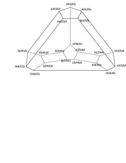
Figure 1: Cyclohedron $W_{4}$.

Proof: (outline) The reader is referred to [B-T], [Mar], [MSS], and [Si] for more detailed presentation and related background facts. We restrict ourselves to a brief explanation of the isomorphism (1), sufficient for intended applications.

The functions $\theta_{i}:S^{1}(n)\rightarrow[0,1]$ and their extensions $\bar{\theta}_{i}:S^{1}[n]\rightarrow[0,1]$ can be used as “coordinate functions” on spaces $S^{1}(n)$ and $S^{1}[n]$ respectively. They can be combined to create $2$-dimensional, $3$-dimensional, or higher dimensional “navigation instruments”, with the corresponding screens being one, two, or higher dimensional simplices $\Delta^{2},\Delta^{3}$ etc. For example, given a $4$-element subconfiguration $q_{i}\prec q_{j}\prec q_{k}\prec q_{l}$ of $q=\{q_{1}\prec\ldots\prec q_{n}\}$, one can extend the function $\lambda:S^{1}(n)\rightarrow\Delta^{2}$ defined by

$$\lambda(q):=\frac{1}{\measuredangle(q_{i},q_{l})}(\measuredangle(q_{i},q_{j}),\measuredangle(q_{j},q_{k}),\measuredangle(q_{k},q_{l}))$$ (2)

to a function $\bar{\lambda}:S^{1}[n]\rightarrow\Delta^{2}$, where $\measuredangle(p,q)=\widehat{p\,q}$ is the arc length of the (counterclockwise) arc with endpoints $p$ and $q$. Indeed, the function $\lambda$ can be expressed in terms of functions $\theta_{i}$, consequently it can be extended to $S^{1}[n]$ and its extension similarly expressed in terms of functions $\bar{\theta}_{i}$.

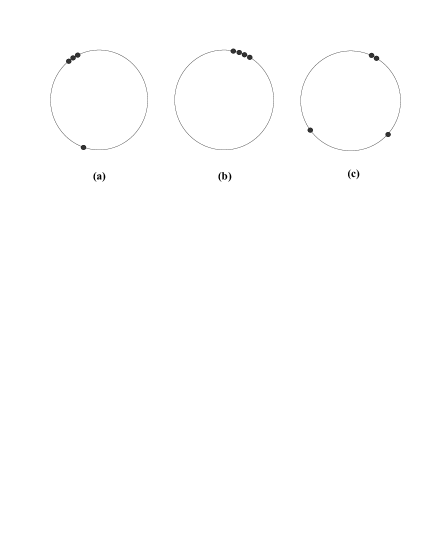
Figure 2: Generic configurations in $\partial W_{4}$.

The configuration space $S^{1}(n)$ is clearly isomorphic to $S^{1}\times{\rm Int}(\Delta)^{n-1}$. The reader can use the “navigation screens” to convince herself that the compactification of this space is indeed described by equation (1). For example one can check that the generic configurations depicted in Figure 2 (a), (b), and (c), respectively correspond to parallelograms, pentagonal, and hexagonal facets of the cyclohedron $W_{4}$. $\square$

Figure 3: Cyclohedron as a compactification/truncation of a simplex.

5 Square pegs in round holes

We begin with a version of the “square pegs in round holes” theorem for $C^{1}$-smooth curves embedded in the $2$-space. This result was in this generality proved by Stromquist [St], see also Schnirelmann [Shn] and Guggenheimer [Gug] for earlier results established with some extra hypotheses on the smoothness or curvature of the curve. The reader is referred to [Grü] (p. 84) for a list of references addressing the case of a convex curve and to [Pa08] for what appears to be the only elementary presentation of the case of simple closed polygons.

Theorem 5.

Every simple closed curve $\Gamma\subset\mathbb{R}^{2}$, which is $C^{1}$-smooth, i.e. has a non-vanishing and continuously moving tangent vector at each point, admits an inscribed square.

Our proof of Theorem 5 serves as a model for other proofs of similar nature. For this reason it is broken into relevant individual steps illustrating FMASK-compactification modification of the usual $CS/TM$-scheme [Ž04]. The scheme of the proof is summarized in Section 5.5.

Theorem 5 is a not the most general result about inscribed squares in Jordan curves, see [St], and Section 8 for a related discussion from the FMASK-compactification point of view.

5.1 Configuration space $S^{1}(4)$ and the test maps

Suppose that $f:S^{1}\rightarrow\mathbb{R}^{2}$ is a smooth embedding satisfying the conditions of Theorem 5. Moreover we silently assume, here and elsewhere in the paper, that the embedding is “counterclockwise” in the sense that the degree of the associated map $s\mapsto df/ds$ is $+1$.

Let $\Gamma={\rm Image}(f)\subset\mathbb{R}^{2}$ be the associated smooth curve. Suppose that $U:=U_{1}\oplus U_{2}\oplus U_{3}$ is a vector space such that $U_{1}\cong\mathbb{R}^{2},U_{2}\cong U_{3}\cong\mathbb{R}$ and let $\Phi:(S^{1})^{4}\rightarrow U$ be the map defined by

$$\Phi(t)=(\phi_{1}(F(t)),\phi_{2}(F(t)),\phi_{3}(F(t)))$$ (3)

where $F:=f^{\times 4}:(S^{1})^{4}\rightarrow\mathbb{R}^{2}\oplus\mathbb{R}\oplus\mathbb{R}$ is the map induced by $f$ and

$$\begin{array}[]{l}\phi_{1}(y)=\frac{y_{1}+y_{3}}{2}-\frac{y_{2}+y_{4}}{2},\\ \phi_{2}(y)=\|y_{1}-y_{3}\|-\|y_{2}-y_{4}\|,\\ \phi_{3}(y)=\|y_{1}-y_{2}\|-\|y_{2}-y_{3}\|+\|y_{3}-y_{4}\|-\|y_{4}-y_{1}\|.\end{array}$$

It is clear that $f(t_{1}),f(t_{2}),f(t_{3}),f(t_{4})$ are consecutive vertices of a square inscribed in the curve $\Gamma$ if and only if $\Phi(t)=0$.

Let $\Phi_{0}:S^{1}(4)\rightarrow U$ be the restriction of $\Phi$ on the configuration space $S^{1}(4)$ of all labelled $4$-element subsets of $S^{1}$ such that the labelling agrees with the counterclockwise (cyclic) order of points on the circle $S^{1}$.

The symmetric group $S_{4}$ acts on $(S^{1})^{4}$ by permuting coordinates. However, it is its subgroup $\mathbb{Z}/4$ of cyclic permutations that naturally acts on $U$ and its subspaces $U_{i}$, and turns $\Phi$ into a $\mathbb{Z}/4$-equivariant map. In turn $\Phi_{0}$ is also a $\mathbb{Z}/4$-equivariant map and for the proof of Theorem 5 it would be sufficient to show that such an equivariant map must have a zero.

Finally, let us record for the further reference that the generator $\omega\in\mathbb{Z}/2$ acts on $S^{1}[4]=S^{1}\times W_{4}$ by reversing the orientation while the action on $U$ is the antipodal action $\omega(v)=-v$, hence it preserves the orientation of $U\cong\mathbb{R}^{4}$.

5.2 Compactified configuration space $S^{1}[4]$

Let $S^{1}[4]$ be the canonical or FMASK-compactification of the configuration space $S^{1}(4)$. We use the basic properties of this compactification, as outlined in Section 3, to define a modified test map ${\Psi}_{0}:S^{1}[4]\rightarrow U$.

Let $\eta:(S^{1})^{4}\rightarrow\mathbb{R}$ be the map defined on the configuration $t=(t_{1},t_{2},t_{3},t_{4})\in(S^{1})^{4}$ as the arc-length diameter of the set $\{t_{1},t_{2},t_{3},t_{4}\}$, i.e. the minimum arc-length of a closed arc $L\subset S^{1}$ such that $t_{i}\in L$ for each $i$. Let $\xi:=\eta^{-1}$ and let $\Phi^{\prime}$ be the modification of the test map $\Phi$ (equation (3)) defined by

$$\Phi^{\prime}(t):=\xi(t)\cdot\Phi(t)=(\xi(t)\phi_{1}(F(t)),\xi(t)\phi_{2}(F(t)),\xi(t)\phi_{3}(F(t))).$$ (4)

Finally, let $\Phi_{0}^{\prime}$ be the restriction of $\Phi_{0}$ on $S^{1}(4)$.

Proposition 6.

The $\mathbb{Z}/4$-equivariant map $\Phi_{0}^{\prime}:S^{1}(4)\rightarrow U$ can be extended to a $\mathbb{Z}/4$-equivariant map $\Psi:S^{1}[4]\rightarrow U$ such that $\Psi(x)\neq 0$ for each $x\in S^{1}[4]\setminus S^{1}(4)\cong S^{1}\times\partial W_{4}$. Moreover, the $\mathbb{Z}/4$-equivariant homotopy class of the restriction $\Psi^{\partial}:S^{1}\times\partial W_{4}\rightarrow U\setminus\{0\}$ does not depend on the embedding $f:S^{1}\rightarrow\mathbb{R}^{2}$.

Proof: The extension $\Psi$ is clearly unique (if it exists). It is also clear that the only case to be discussed is the case of points $q\in S^{1}[4]\setminus S^{1}(4)$ such that $\eta(q)=0$, or equivalently $\xi(q)=+\infty$. These are the points which corresponds to pentagons in Figure 1 and can be characterized as limits in $S^{1}[4]$ of sequences $q_{n}=\{t_{i}^{n}\prec t_{j}^{n}\prec t_{k}^{n}\prec t_{l}^{n}\}$, where $(i,j,k,l)$ is a cyclic permutation of elements $\{1,2,3,4\}$ and $\measuredangle(t_{i}^{n},t_{l}^{n})\mapsto 0$ as $n\mapsto+\infty$. The last condition implies that all sequences $(t_{i}^{n})_{n=1}^{+\infty}$ converge to the same point $s\in S^{1}$.

The point $q\in S^{1}[4]$, which is the limit (in $S^{1}[4]$) of the sequence $q_{n}\in S^{1}(4)$, is (in the language of Section 4) best visualized in the $2$-dimensional screens described by equation (2). Since the associated barycentric coordinates $\frac{\measuredangle(t_{i}^{n},t_{j}^{n})}{\measuredangle(t_{i}^{n},t_{l}^{n})}$ etc. are all well defined as functions on $S^{1}[4]$, it remains to be checked that the same applies to the functions $\frac{\phi_{i}(F(t))}{\eta(t)}$ that appear in the test map (4), i.e. that these quotient can be meaningfully (and continuously) extended to points $q\in S^{1}[4]$. Since in the small neighborhood of $s\in S^{1}$ the function $f:S^{1}\rightarrow\mathbb{R}^{2}$ is approximated by a linear function, i.e. the curve $\Gamma$ is in the vicinity of $z=f(s)$ (up to a higher order infinitesimal) approximated by its tangent line at $z\in\Gamma$, we make the following useful observation.

1. The value of the test function $\Psi=(\Psi_{1},\Psi_{2},\Psi_{3})$ at a point $q\in S^{1}[4]$ is equal to the value of the original test function $\Phi_{0}$ at an “infinitesimal” quadruple $q_{n}=\{t_{i}^{n}\prec t_{j}^{n}\prec t_{k}^{n}\prec t_{l}^{n}\}$ approximating $q$, divided by the associated “infinitesimal” arc-length $\eta(q_{n})$.

It follows that $\Psi_{1}(q)$ is always a non-zero vector collinear to the tangent vector of $\Gamma$ at $z=f(s)$ with the only exception being the case of the point $q$ represented by an “infinitesimal parallelogram” i.e. if

$$\lim_{n\mapsto\infty}\frac{\measuredangle(t_{i}^{n},t_{j}^{n})}{\measuredangle(t_{i}^{n},t_{k}^{n})}=\lim_{n\mapsto\infty}\frac{\measuredangle(t_{k}^{n},t_{l}^{n})}{\measuredangle(t_{j}^{n},t_{l}^{n})}=0.$$

In this case it is not difficult to check that $\Psi_{3}(q)\neq 0$ which comletes the proof of the first part of the proposition.

For the second part, let us suppose that $f_{0},f_{1}:S^{1}\rightarrow\mathbb{R}^{2}$ are two smooth embeddings such that both maps $s\mapsto df_{i}/ds,\,i=0,1$ have degree $+1$. Then the independence of the $\mathbb{Z}/4$-homotopy class of the map $\Psi^{\partial}$ from the embedding $f:S^{1}\rightarrow\mathbb{R}^{2}$ follows from the fact that any two such embeddings can be connected by a regular homotopy i.e. by a family $f_{t},\,t\in[0,1]$ of smooth embeddings such $df_{t}(s)/ds\neq 0$ for each $s\in S^{1}$. $\square$

5.3 The obstruction $\ldots$

It remains to be shown that no map in the $\mathbb{Z}/4$-equivariant homotopy class of the map $\Psi^{\partial}$ can be extended to $S^{1}\times W_{4}$, i.e. that there does not exist a $\mathbb{Z}/4$-equivariant map “?” that completes the square

$$\begin{CD}S^{1}\times\partial(W_{4}))@>{\Psi^{\partial}}>{}>S^{3}\\ @V{}V{}V@V{}V{\cong}V\\ S^{1}\times W_{4}@>{?}>{}>S^{3}\end{CD}$$ (5)

The obstruction to the extension problem (5) lives in the equivariant cohomology group

$$H^{4}_{\mathbb{Z}/4}((S^{1}\times W_{4}),S^{1}\times\partial(W_{4}));\mathcal{Z}))$$

where $\mathcal{Z}=\pi_{3}(U\setminus\{0\})\cong H_{3}(U\setminus\{0\})\cong H_{3}(S^{3})\cong\mathbb{Z}$ inherits the $\mathbb{Z}/4$-module structure from the $\mathbb{Z}/4$-action on $U$. By equivariant Poincaré duality this group is isomorphic to the group

$$H_{0}^{\mathbb{Z}/4}((S^{1}\times W_{4})\setminus S^{1}\times\partial(W_{4}));\mathcal{Z}\otimes\varepsilon))\cong\mathcal{Z}_{\mathbb{Z}/4}\cong\mathbb{Z}/2$$

where $\varepsilon$ is associated orientation character, i.e. the $\mathbb{Z}/4$-module $H_{4}(S^{1}[4],\partial S^{1}[4];\mathbb{Z})$.

5.4 $\ldots$ and its evaluation

We evaluate the obstruction in $\mathcal{Z}_{\mathbb{Z}/4}\cong\mathbb{Z}/2$ by counting the zeros of a “generic” (transverse to zero) map $?:S^{1}\times W_{4}\rightarrow U$ (diagram (5)) which extends a map in the $\mathbb{Z}/4$-equivariant homotopy class of $\Psi^{\partial}$.

Suppose that $\Gamma$ is a smooth oval in the plane which admits a $\mathbb{Z}/2\times\mathbb{Z}/2$ symmetry. For example we can choose for $\Gamma$ the ellipse centered at the origin, symmetric with respect to the coordinate axes (Figure 4). Such an oval (ellipse) has a unique inscribed square. Suppose that the vertices of this square (in counterclockwise order) are $b_{1},b_{2},b_{3},b_{4}$ and that $b_{1}$ is in the first quadrant. Moreover we assume that $b_{j}=f(a_{j})$ for some parameters $a_{j}\in S^{1}$.

There is an obvious isomorphism $T_{a}(S^{1}(4))\cong\oplus_{i=1}^{4}~{}T_{a_{i}}(S^{1})$ of tangent spaces. Let $x_{i}$ be a local coordinate on $S^{1}$ defined in the neighborhood of $a_{i}$. For example let $x_{i}(c)$ be the (oriented) angle $\measuredangle(a_{i},c)$ swept by the radius vector moving from $a_{i}$ to $c$. Let $[\frac{\partial}{\partial x_{j}}]_{j=1}^{4}=[\frac{\partial}{\partial x_{1}},\frac{\partial}{\partial x_{2}},\frac{\partial}{\partial x_{3}},\frac{\partial}{\partial x_{4}}]$ be the associated basis (frame) of tangent vectors in $T_{a}(S^{1}(4))$.

We want to show that the differential $d\Psi_{a}:T_{a}(S^{1}(4))\rightarrow T_{0}(\mathbb{R}^{4})\cong\mathbb{R}^{4}$ of $\Psi$, evaluated at $a=(a_{1},a_{2},a_{3},a_{4})$, is non-degenerate. Let $y_{i}:=x_{i}\circ f^{-1}$ be the local coordinate on $\Gamma$ defined in the neighborhood of $b_{i}$, induced by $x_{i}$. It follows that the differential $dF_{a}:T_{a}((S^{1})^{4})\rightarrow T_{b}(\Gamma^{4})$ maps the frame $[\frac{\partial}{\partial x_{j}}]_{j=1}^{4}$ to $[\lambda_{j}\frac{\partial}{\partial y_{j}}]_{j=1}^{4}$, for appropriate non-zero scalars $\lambda_{j}$.

Let $\alpha:(\mathbb{R}^{2})^{4}\rightarrow\mathbb{R}^{2}\times\mathbb{R}\times\mathbb{R}$ be the map defined by $\alpha(y)=(\phi_{1}(y),\phi_{2}(y),\phi_{3}(y))$, so in particular $\Phi(x)=\alpha(F(x))$.

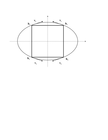
Figure 4:

The frame $[\frac{\partial\Psi}{\partial x_{j}}]_{j=1}^{n}=[d\Psi(\frac{\partial}{\partial x_{j}})]_{j=1}^{4}$ is equal, up to rescaling and possibly up to some changes of signs, to the frame $[d\alpha(v_{i})]_{i=1}^{4}$ where $v_{i}$ is an arbitrary (non-zero) vector in $T_{b_{i}}(\Gamma)$ prescribed in advance. For convenience (Figure 4) we assume that the collection $\{v_{i}\}_{i=1}^{4}$ is also $(\mathbb{Z}/2\times\mathbb{Z}/2)$-invariant.

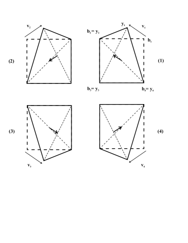
Figure 5:

Let us suppose that the rate of change of $\alpha$ in the direction of vector $v_{1}$, evaluated at the point $(b_{1},b_{2},b_{3},b_{4})$, is

$$d\alpha(v_{1})=d\alpha_{b}(v_{1})=(u;s,t)=(u_{1},u_{2};s,t)\in\mathbb{R}^{2}\oplus\mathbb{R}\oplus\mathbb{R}.$$

By taking into account the $(\mathbb{Z}/2\times\mathbb{Z}/2)$-symmetry of the curve $\Gamma$, one easily deduces that

$$\begin{array}[]{cccccccc}d\alpha(v_{2})&=&(u_{1},-u_{2};-s,t)&&&d\alpha(v_{1})&=&(u_{1},u_{2};s,t)\\ d\alpha(v_{3})&=&(-u_{1},-u_{2};s,t)&&&d\alpha(v_{4})&=&(-u_{1},u_{2};-s,t).\end{array}$$

It follows that the determinant $Det$ of the frame $[d\alpha(v_{j})]_{j=1}^{4}$ is

$$Det=\left|\begin{array}[]{lrrr}u_{1}&u_{1}&-u_{1}&-u_{1}\\ u_{2}&-u_{2}&-u_{2}&u_{2}\\ s&-s&s&\!-s\\ t&t&t&\!t\end{array}\right|=-16stu_{1}u_{2}\neq 0$$

which in turn implies that the frame $[\frac{\partial\Psi}{\partial x_{j}}]_{j=1}^{4}$ is also non-degenerate.

5.5 The proof of Theorem 5

Proof of Theorem 5: Assume that $f:S^{1}\rightarrow\mathbb{R}^{2}$ is a (counterclockwise) smooth parametrization of the curve $\Gamma$. The zeros of the associated ($\mathbb{Z}/4$-equivariant) “test map” $\Phi_{0}:S^{1}(4)\rightarrow U$ (Section 5.1) are in one-to-one correspondence with the squares inscribed in $\Gamma$. After rescaling by a suitable positive, real function $\xi$, the modified test map $\Phi_{0}^{\prime}:=\xi\Phi_{0}$ is $\mathbb{Z}/4$-equivariantly extended (Section 5.2) to a map $\Psi:S^{1}[4]\rightarrow U$, where $S^{1}[4]$ is the Fulton-MacPherson compactification of $S^{1}(4)$. The restriction $\Psi^{\partial}$ of $\Psi$ on the boundary $\partial S^{1}[4]$ of $S^{1}[4]$ has no zeros (Proposition 6). Moreover, its $\mathbb{Z}/4$-equivariant homotopy class is independent of the original curve $\Gamma$. The obstruction for extending $\mathbb{Z}/4$-equivariantly the map $\Psi^{\partial}:\partial S^{1}[4]\rightarrow U\setminus\{0\}$ to $S^{1}[4]$ is found to be non-trivial (Sections 5.3 and 5.4) which finally implies that $\Phi_{0}$ must have a zero in $S^{1}(4)$. $\square$

6 Grünbaum’s conjecture

B. Grünbaum, see [Grü] page 85, conjectured that every Jordan curve in the plane contains the vertices of an affine-regular hexagon. By definition a hexagon in the plane is affine-regular if it is the image of a regular hexagon by an affine automorphism of the plane. In contrast to the square peg problem, as emphasized in [Grü], the Grünbaum’s conjecture has been opened even for the case of smooth curves. In this section we establish this case of the conjecture and refer the reader to Section 8 for a brief discussion how the smoothness condition can be relaxed.

Theorem 7.

Every $C^{1}$-smooth, simple, closed curve in the plane contains either the vertices of an affine-regular hexagon or six collinear points which are the limit configuration of a convergent sequence of affine-regular hexagons.

The proof of Theorem 7 follows the same scheme used in Section 5 so we focus our attention on differences and relevant calculations. By assumption $\Gamma\subset\mathbb{R}^{2}$ is a simple, closed, $C^{1}$-smooth curve in the plane, the last condition saying that a parametrization can be chosen so that the curve has a non-zero, continuously moving tangent vector.

In analogy with the square peg problem we choose for the configuration space the Fulton-MacPherson compactification $S^{1}[6]$ of the space $S^{1}(6)$ of all labelled, cyclically ordered $6$-element subsets $\{t_{1}\prec t_{2}\prec\ldots\prec t_{6}\prec t_{1}\}$ in $S^{1}$. Next we introduce the maps $\alpha,\beta,\gamma,\delta$ which serve for testing if the points $x_{1},x_{2},\ldots,x_{6}$ are consecutive vertices of an affine-regular hexagon in the plane,

$$\begin{array}[]{l}\alpha(x)=x_{1}+x_{4}-x_{2}-x_{5}\\ \beta(x)=x_{2}+x_{5}-x_{3}-x_{6}\\ \gamma(x)=x_{3}+x_{6}-x_{1}-x_{4}\\ \delta(x)=x_{1}-x_{2}+x_{3}-x_{4}+x_{5}-x_{6}.\end{array}$$ (6)

Note that the condition $\alpha(x)=0$ says that the midpoints of the large diagonals $[x_{1},x_{4}]$ and $[x_{2},x_{5}]$ coincide while $\delta(x)=0$, in addition to $\alpha(x)=\beta(x)=\gamma(x)=0$, guarantees that the pairs of opposite sides are parallel to and half the length of the large diagonal separating them.

As in the “square peg problem”, the system of equations

$$\alpha(x)=\beta(x)=\gamma(x)=\delta(x)=0,$$ (7)

admits, aside from genuine affine-regular hexagons, also some degenerate solutions, for example the hexagons where all vertices collapse to the same point. More generally there exist solutions where points coincide in pairs, e.g. the solution $x_{1}=x_{2}=a,x_{4}=x_{5}=-a,x_{3}=x_{6}$ and the solutions obtained from this one by a cyclic permutation of indices. These two types of degenerate solutions will be referred to as $1$-point and $3$-point degenerate solutions. The system (7) has also collinear $6$-point solutions and together these are the only degenerate solutions that can occur. In order to understand better these $6$-point “pseudo-solutions”, let us assume that $x_{1}+x_{3}+x_{5}=x_{2}+x_{4}+x_{6}=0$ and that all these points belong to the real axes. In light of the fact that $x_{1}+x_{3}=x_{2},x_{2}+x_{4}=x_{3}$, etc. we see that if $0<x_{2}<x_{1}$ then $x_{3}<0$ (Figure 6) which leads to the following simple but important observation.

Observation 8.

Suppose that $x_{1},x_{2},\ldots,x_{6}$ are collinear points which are also vertices of a degenerate, affine-regular hexagon, i.e. a configuration obtained as a limit of a convergent sequence of affine-regular hexagons. Suppose that these points appear in this order on a smooth, Jordan curve $\Gamma$, i.e. $x_{j}=f(t_{j})$ where $t_{1}\prec t_{2}\prec\ldots\prec t_{6}\prec t_{1}$. Then the order of the appearance of these points on the line (in any direction) is a non-trivial permutation of indices $1,2,\ldots,6$ different from a cyclic permutation.

Figure 6: A degenerate, affine-regular hexagon.

6.1 Compactified configuration space and the test maps

Let $U^{\prime}\cong U_{1}^{3}\oplus U_{2}$, where $U_{1}\cong U_{2}\cong\mathbb{R}^{2}$, be the preliminary test space defined as the total target space for the test maps $\alpha,\beta,\gamma$ and $\delta$, described in (6). Since the first three maps are not independent $\alpha+\beta+\gamma=0$, let $V:=\{(u,v,w)\in U_{1}^{3}\mid u+v+w=0\}$ and let the actual “test space” be the direct sum $U=V\oplus U_{2}\subset U^{\prime}$. Let $F:(S^{1})^{6}\rightarrow(\mathbb{R}^{2})^{6}$ be the map induced by the embedding $f:S^{1}\rightarrow\mathbb{R}^{2}$ and $\Phi:(S^{1})^{6}\rightarrow U$ the “test map” where $\Phi(t):=(\alpha(F(t)),\beta(F(t)),\gamma(F(t)))\oplus(\delta(F(t)))$. Finally, let $\Phi_{0}:S^{1}(6)\rightarrow U$ be the restriction of $\Phi$ on the configuration space $S^{1}(6)$.

The next step, as in Section 5.2, is a rescaling of the map $\Phi_{0}$ in order to make it suitable for an extension on the compactified configuration space $S^{1}[6]$. As before (Section 5.2) let $\eta:S^{1}(6)\rightarrow\mathbb{R}^{+}$ be the map evaluating the “circular diameter” of a configuration $t_{1}\prec t_{2}\prec\ldots\prec t_{6}\in S^{1}(6)$ and $\xi:=\eta^{-1}$. Let $\Phi^{\prime}:=\xi\cdot\Phi$ be the rescaled version of the map $\Phi$ and $\Phi_{0}^{\prime}$ its restriction on $S^{1}(6)$.

The proof of the following proposition is similar to the proof of Proposition 6 so we omit most of the details.

Proposition 9.

The $\mathbb{Z}/6$-equivariant map $\Phi_{0}^{\prime}:S^{1}(6)\rightarrow U$ can be extended to a $\mathbb{Z}/6$-equivariant map $\Psi:S^{1}[6]\rightarrow U$ such that $\Psi(x)\neq 0$ for each $x\in S^{1}[6]\setminus S^{1}(6)\cong S^{1}\times\partial W_{6}$. Moreover, the $\mathbb{Z}/6$-equivariant homotopy class of the restriction $\Psi^{\partial}:S^{1}\times\partial W_{6}\rightarrow U\setminus\{0\}$ does not depend on the (counterclockwise) embedding $f:S^{1}\rightarrow\mathbb{R}^{2}$.

Proof: (outline) In order to show that $\Psi$ has no zeros on the boundary $S^{1}\times\partial W_{6}$ we have to show that “infinitesimal degenerate hexagons” cannot appear as zeros of the map $\Psi:S^{1}[6]\rightarrow U$. Indeed, this is ruled out by the Observation 8. The rest of Proposition 9 is established by the arguments already used in the proof of Proposition 6 so we omit the details. $\square$

6.2 The obstruction and its evaluation

As in Section 5.3, there arises an extension problem

$$\begin{CD}S^{1}\times\partial(W_{6}))@>{\Psi^{\partial}}>{}>S^{5}\\ @V{}V{}V@V{}V{\cong}V\\ S^{1}\times W_{6}@>{?}>{}>S^{5}\end{CD}$$ (8)

with the corresponding obstruction living in the group

$$H^{6}_{\mathbb{Z}/6}((S^{1}\times W_{6}),S^{1}\times\partial(W_{6}));\mathcal{Z}))\cong H_{0}^{\mathbb{Z}/6}((S^{1}\times W_{6})\setminus S^{1}\times\partial(W_{6}));\mathcal{Z}))\cong\mathcal{Z}_{\mathbb{Z}/6}\cong\mathbb{Z}/2.$$

As in Section 5.3 we evaluate the obstruction by choosing a conveniently “generic” curve $\Gamma\subset\mathbb{R}^{2}$ and counting the number of affine-regular hexagons inscribed in this curve.

Figure 7:

Let $\Gamma$ be the boundary of a triangle (Figure 7). In order to make it a smooth curve one is allowed to round its corners, however this will not affect the calculations.

As it is clear from the picture there is only one affine-regular hexagon inscribed in this curve. It remains to be shown, as in Section 5.4, that a neighborhood of this hexagon is mapped by the test map to a neighborhood of $0$, i.e. that $0$ is a regular point of the test map $\Psi$.

Assume that $x_{1},x_{2},\ldots,x_{6}$ are local coordinates (on the configuration space $\Gamma(6)\cong S^{1}(6)$), in the neighborhood of the hexagon depicted in Figure 7. More precisely $x_{1}$ is a point in the neighborhood of $x_{1}^{0}$, constrained to move only on the $BC$ side of the triangle, similarly $x_{2},\ldots,x_{6}$ are perturbations of respective points $x_{2}^{0},\ldots,x_{6}^{0}$ allowed to move only on the boundary of the triangle.

It follows, since the function $\gamma$ can be expressed in terms of $\alpha$ and $\beta$, that we have to compute and establish the non-triviality of the Jacobian $J$ of the map $x=(x_{1},x_{2},\ldots,x_{6})\mapsto(\alpha(x),\beta(x),\delta(x))$, evaluated at the point $(x_{1}^{0},\ldots,x_{6}^{0})$.

By inspection, and up to some rescaling of vectors $\overrightarrow{AB},\overrightarrow{BC},\overrightarrow{CA}$, the Jacobian matrix is found to have the following form:

$$J=\begin{array}[]{r|cccccc}&x_{1}&x_{2}&x_{3}&x_{4}&x_{5}&x_{6}\\ \hline\cr\vspace{-3mm}\hfil&&&&&&\\ \alpha&{\small\overrightarrow{BC}}&-{\small\overrightarrow{BC}}&0&{\small\overrightarrow{CA}}&-{\small\overrightarrow{AB}}&0\vspace{1mm}\\ \beta&0&{\small\overrightarrow{BC}}&-{\small\overrightarrow{CA}}&0&{\small\overrightarrow{AB}}&{\small\overrightarrow{-AB}\vspace{1mm}}\\ \delta&{\small\overrightarrow{BC}}&-{\small\overrightarrow{BC}}&{\small\overrightarrow{CA}}&-{\small\overrightarrow{CA}}&{\small\overrightarrow{AB}}&-{\small\overrightarrow{AB}}\end{array}$$ (9)

Finally, by choosing $\overrightarrow{BC},\overrightarrow{CA}$ and $\overrightarrow{AB}$ to be respectively the column vectors of the matrix

$$\left[\begin{array}[]{crr}1&-1&0\\ 0&1&-1\end{array}\right]$$

we obtain a matrix with the determinant equal to $3$. This calculation confirms that the hexagon depicted in Figure 7 is indeed a non-degenerate solution of the system of equations (7) which in turn implies that the obstruction to the extension problem (8) is a non-trivial element of the group $\mathcal{Z}_{\mathbb{Z}/6}\cong\mathbb{Z}/2$. $\square$

7 Hadwiger’s conjecture

Conjecture 10.

([Ha]) Every simple closed curve in the Euclidean $3$-space contains four distinct points which are the vertices of a parallelogram.

Relying on the same method as in the previous sections we establish a stronger statement (at least for $C^{1}$-smooth curves) that this parallelogram can be claimed to have all sides pairwise equal i.e. to be a rhombus. As it turned out this theorem was already established by Makeev in [Mak] whose initial motivation was the question of inscribing equilateral polygonal lines in space curves.

Theorem 11.

([Mak]) Every $C^{1}$-smooth simple closed curve $\Gamma$ immersed in the Euclidean $3$-space contains the vertices of a rhombus.

Proof: By assumption the curve $\Gamma\subset\mathbb{R}^{3}$ admits a $C^{1}$-parametrization. In other words it can be parameterized by an injective $C^{1}$-mapping $\varphi:S^{1}\to\mathbb{R}^{3}$ such that the tangent vector $d\varphi/dt$ is nowhere zero, continuous function of $t$.

As before $S^{1}(4)$ is the configuration space of cyclically ordered four-tuples of distinct points on the circle. Given a point $(t_{1}\prec t_{2}\prec t_{3}\prec t_{4})\in S^{1}(4)$, let $x_{i}=\varphi(t_{i})$ for $i=1,2,3,4$. Let $\Gamma(4):={\rm Image}(\Phi)$ where $\Phi:S^{1}(4)\rightarrow(\mathbb{R}^{3})^{4}$ is the map induced by $\varphi$.

Define a test map $F=F_{\varphi}:S^{1}(4)\to\mathbb{R}^{4}$ as the composition $F:=\Psi\circ\Phi$ where $\Psi=(\Psi_{1},\Psi_{2}):(\mathbb{R}^{3})^{4}\rightarrow\mathbb{R}^{3}\oplus\mathbb{R}$ is described by equations:

$$\begin{array}[]{lcl}\Psi_{1}(x)&=&x_{1}-x_{2}+x_{3}-x_{4}\\ \Psi_{2}(x)&=&\|x_{1}-x_{2}\|-\|x_{2}-x_{3}\|+\|x_{3}-x_{4}\|-\|x_{4}-x_{1}\|.\end{array}$$ (10)

For a given input $x=(x_{1},x_{2},x_{3},x_{4})\in\mathbb{R}^{4}$, the first function $\Psi_{1}(x)$ describes a point in $\mathbb{R}^{3}$ which is equal to $0$ if and only if the mid-points of the diagonals of the quadrilateral with the vertices $x_{1},x_{2},x_{3},x_{4}$ coincide (i.e. if it is a parallelogram). If in addition the second function $\Psi_{2}$ is equal to $0$, then such a parallelogram have all sides equal (i.e. it is a rhombus). This shows that the rhombuses inscribed in the curve $\Gamma$ correspond to zeros of the test map $F=F_{\varphi}$.

Let $S^{1}[4]\cong S^{1}\times W_{4}$ be the Fulton-MacPherson compactification of the configuration space $S^{1}(4)$. As in the previous sections one can extend, after some rescaling, the function $F$ to a function $\tilde{F}=\tilde{F}_{\varphi}:S^{1}[4]\to\mathbb{R}^{4}$. More explicitly, if $\eta(t)$ is the arc-length diameter of the set $t=\{t_{1},t_{2},t_{3},t_{4}\}\subset S^{1}$ and $\xi(t):=\eta(t)^{-1}$ then $\tilde{F}$ is the extension of the map $\xi\cdot F:S^{1}(4)\rightarrow\mathbb{R}^{4}$.

The group $\mathbb{Z}/4$ acts on the configuration space $S^{1}(4)$ by cyclic permutations and this action could be extended to its compactification $S^{1}[4]$. Moreover, both the test map $F_{\varphi}$ and its extension $\tilde{F}_{\varphi}$ are $\mathbb{Z}/4$-equivariant. The target space $\mathbb{R}^{4}\cong U_{1}\oplus U_{2}$ naturally splits as the sum of a $3$-dimensional and a $1$-dimensional, real $\mathbb{Z}/4$-representation.

Proposition 12.

The restriction $\tilde{F}_{\varphi}^{\partial}$ of the map $\tilde{F}_{\varphi}$ on the boundary $S^{1}\times\partial(W_{4})$ of $S^{1}[4]=S^{1}\times W_{4}$ has no zeros. Moreover, the $\mathbb{Z}/4$-equivariant homotopy class of the restriction $\tilde{F}_{\varphi}^{\partial}:S^{1}\times\partial(W_{4})\rightarrow\mathbb{R}^{4}\setminus\{0\}$ depends neither on the curve $\Gamma$ nor on its $C^{1}$-parametrization $\varphi$.

Proof: Let $\tilde{F}_{\varphi}^{1}:S^{1}\times\partial(W_{4})\rightarrow U_{1}$ and $\tilde{F}_{\varphi}^{2}:S^{1}\times\partial(W_{4})\rightarrow U_{2}$ be the components of the map $\tilde{F}_{\varphi}^{\partial}=(\tilde{F}_{\varphi}^{1},\tilde{F}_{\varphi}^{2}):S^{1}\times\partial(W_{4})\rightarrow U_{1}\oplus U_{2}\cong\mathbb{R}^{4}$. By definition (equation (10)) $\tilde{F}_{\varphi}^{j},\,j=1,2$, is the extension of the map $\xi\cdot(\Psi_{j}\circ\Phi)$.

For the majority of the points $q\in S^{1}\times\partial(W_{4})$ already the function $\tilde{F}_{\varphi}^{1}$ is non-zero. More precisely $\tilde{F}_{\varphi}^{1}(q)$ is zero only if $q$ is a degenerate parallelogram i.e. if $q\in S^{1}\times(I_{1}\cup I_{2})$ where $I_{1}=[(23)(41),(41)(23)]$ and $I_{2}=[(12)(34),(34)(12)]$ are the corresponding edges of the cyclohedron $W_{4}$ depicted in Figure 1. If $q\in I_{1}\cup I_{2}$ then $\tilde{F}_{\varphi}^{2}(q)\neq 0$, which completes the proof of the first part of the proposition.

For the proof of the second part of the proposition let us begin with a simple observation that the $\mathbb{Z}/4$-equivariant homotopy class of $\tilde{F}_{\varphi}^{\partial}$ does not depend on the smooth reparameterization of the curve $\Gamma$. Indeed, such a reparametrization $\alpha:S^{1}\rightarrow S^{1}$ defines a nowhere zero vector field on $S^{1}$, which can be linearly contracted to the zero vector field. Hence, there is a smooth homotopy between $\varphi$ and $\varphi^{\prime}:=\varphi\circ\alpha$ which induces a $\mathbb{Z}/4$-equivariant homotopy between $\tilde{F}_{\varphi}^{\partial}$ and $\tilde{F}_{\varphi^{\prime}}^{\partial}$. Similar argument can be used in the case when two curves (knots) $\Gamma_{\varphi}$ and $\Gamma_{\psi}$ are in the same isotopy class, i.e. if they represent the same knot.

For the general case let us suppose that $\varphi$ and $\psi$ are two $C^{1}$-smooth embeddings (knots) of $S^{1}$ in $\mathbb{R}^{3}$ which are not necessarily $C^{1}$-isotopic. A naive candidate for a $\mathbb{Z}/4$-equivariant homotopy between $\tilde{F}_{\varphi}^{\partial}$ and $\tilde{F}_{\psi}^{\partial}$ is the linear homotopy

$$G:S^{1}[4]\times[0,1]\rightarrow\mathbb{R}^{4}$$ (11)

defined by $G(q,t)=(G^{1}(q,t),G^{2}(q,t)):=(1-t)\tilde{F}_{\varphi}^{\partial}+(1-t)\tilde{F}_{\psi}^{\partial}$.

1. Observation 1: The second component $G^{2}$ of the linear homotopy is non-zero on $A=S^{1}\times(I_{1}\cup I_{2})$. Indeed, the signs of both $\tilde{F}_{\varphi}^{1}(q)$ and $\tilde{F}_{\psi}^{1}(q)$ (for $q\in A$) are the same, since they depend solely on the labelling of the vertices of the degenerate parallelogram $q$.

It follows from Observation 1 that it is sufficient to define a (nowhere zero) homotopy $G^{1}(q,t)$ for $q\in D:=\partial S^{1}[4]\setminus(S^{1}\times(I_{1}\cup I_{2}))$. If $\bar{F}_{\varphi}^{1},\bar{F}_{\psi}^{1}:D\rightarrow S^{2}$ are the normalized maps associated to $\tilde{F}_{\varphi}^{1}$ and $\tilde{F}_{\psi}^{1}$, where by definition $\bar{F}_{\varphi}^{1}(q):=\tilde{F}_{\varphi}^{1}(q)/\|\tilde{F}_{\varphi}^{1}(q)\|$ and $\bar{F}_{\psi}^{1}(q):=\tilde{F}_{\psi}^{1}(q)/\|\tilde{F}_{\psi}^{1}(q)\|$, then it is sufficient to define a $\mathbb{Z}/4$-equivariant homotopy $\bar{G}^{1}:D\times I\rightarrow S^{2}$ between these two maps.

1. Observation 2: Both maps $\bar{F}_{\varphi}^{1},\bar{F}_{\psi}^{1}$ can be canonically and $\mathbb{Z}/4$-equivariantly factored through the space $\tilde{F}(S^{1},2)$ defined in Example 1 (Section 3). More precisely there exist a “universal” $(\mathbb{Z}/4\mapsto\mathbb{Z}/2)$-equivariant map $\chi:D\rightarrow\tilde{F}(S^{1},2)$ and $\mathbb{Z}/2$-equivariant maps $\alpha,\beta:\tilde{F}(S^{1},2)\rightarrow S^{2}$ such that $\bar{F}_{\varphi}^{1}=\alpha\circ\chi$ and $\bar{F}_{\psi}^{1}=\beta\circ\chi$.

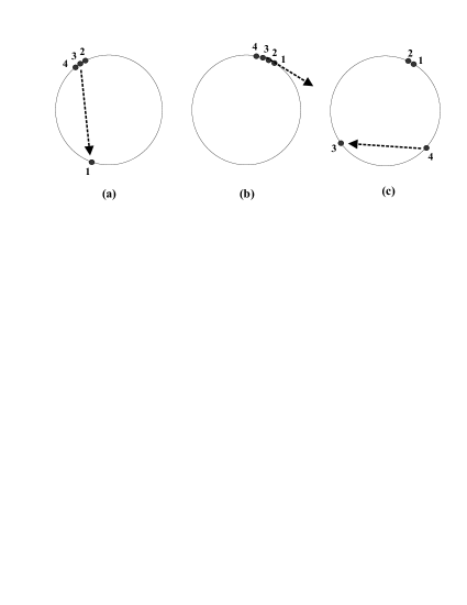
Figure 8: The definition of the map $\chi$.

The definition of the map $\chi$ is quite natural and motivated by the definition of the map $\bar{F}_{\varphi}^{1}$ in the case when $\varphi:S^{1}\hookrightarrow\mathbb{R}^{2}\subset\mathbb{R}^{3}$ is essentially the identity map. Pictorially it is described in Figure 8. Let $q_{1}=(x_{1},x_{2},x_{3},x_{4})$ be a point in $\partial S^{1}[4]$. Generic examples are depicted in Figure 8 (where for simplicity $x_{j}$ is labelled by $j$).

Recall that a point $\tilde{F}(S^{1},2)$ is either an ordered pair $(x,y)$ of points in $S^{1}$ or a pair $(z,u)$ where $z\in S^{1}$ and $u$ is a unit tangent vector in $T_{z}(S^{1})$. If $q=(x_{1},x_{2},x_{3},x_{4})$ is the configuration depicted in Figure 8 (c), then $\chi(q):=(x_{3},x_{4})$. If $q$ is a point depicted in Figure 8 (a), then $\chi(q):=(x_{1},x_{3})$. Finally if $q$ is a point depicted in Figure 8 (b), then $\chi(q)=(z,u)$ where $z=x_{1}=x_{2}=x_{3}=x_{4}$ and $u$ is the unit tangent vector pointing in he same direction as the vector $x_{1}-x_{2}+x_{3}-x_{4}$.

It is not difficult to show that $\tilde{F}(S^{1},2)$ is, as a $\mathbb{Z}/2$-space, $\mathbb{Z}/2$-homotopy equivalent to the circle $S^{1}$ with the antipodal action. The existence of the $\mathbb{Z}/4$-homotopy $\bar{G}^{1}:D\times I\rightarrow S^{2}$ follows from Observation 2 and the fact that any two $\mathbb{Z}/2$-maps $\alpha,\beta:\tilde{F}(S^{1},2)\rightarrow S^{2}$ are $\mathbb{Z}/2$-homotopic. $\square$

Remark 13.

The fact that the $\mathbb{Z}/4$-equivariant homotopy class of the map $\tilde{F}_{\varphi}^{\partial}$ is the same, whether the curve $\Gamma\subset\mathbb{R}^{3}$ is knotted or not, illustrates the versatility of the “cyclohedron approach” to the problem of finding polygonal pegs inscribed in space curves. This should be compared to the planar case where any two (equally oriented) embeddings are isotopic, hence the required homotopies can be constructed by more direct methods.

7.1 Obstruction and its evaluation

Proof of Theorem 11 (cont.): Equipped with Proposition 12, we proceed as in the earlier sections. The obstruction $O$ for a $\mathbb{Z}/4$-equivariant extension of the (homotopically unique) map $\tilde{F}^{\partial}_{\varphi}:S^{1}\times\partial W_{4}\rightarrow\mathbb{R}^{4}\setminus\{0\}$ to $S^{1}\times W_{4}$ lives in $H_{\mathbb{Z}/4}^{4}(S^{1}[4],\partial S^{1}[4];\mathcal{Z})$, cf. Section 5.3. The Poincaré dual of this class belongs to the dual homology group $H_{0}^{\mathbb{Z}/4}(S^{1}[4];\mathcal{Z}\otimes\epsilon)$ and can be evaluated by a careful choice of the curve $\Gamma$.

Let us consider the curve $\Gamma=\Gamma_{1}\cup J$ obtained as the union of the non-closed curve $\Gamma_{1}={\rm Im}(\psi)$, where $\psi:[0,2\pi]\to\mathbb{R}^{3}$ is defined by $\psi(t)=(\cos t,\sin t,t)$, and the interval $J$ joining the endpoints $(1,0,2\pi)$ and $(1,0,0)$ of the curve $\Gamma_{1}$. $\Gamma$ is not a smooth curve however, by smoothing the corners, we obtain a smooth curve $\Gamma^{\prime}$ such that a rhombus $(x_{1},x_{2},x_{3},x_{3})$ is inscribed in $\Gamma$ if and only if it is inscribed in $\Gamma^{\prime}$. For this reason we are allowed to use the test map associated to the curve $\Gamma$.

Let $\varphi:[0,4\pi]\rightarrow\mathbb{R}^{3}$ be the parametrization of $\Gamma$ defined by $\varphi(t)=\psi(t)$ for $t\in[0,2\pi]$ and $\varphi(t):=(1,0,4\pi-t)$ for $t\in[2\pi,4\pi]$.

We will show that there is a precisely one rhombus inscribed in the curve $\Gamma$, i.e. a point $x=(x_{1},x_{2},x_{3},x_{4})\in\Gamma(4)$ such that $F_{\varphi}(x)=0$. Moreover, it will be shown that the test map $F=F_{\varphi}$ is transverse to $0\in\mathbb{R}^{4}$, i.e. that $0$ is a regular value of $F$.

The only way to have two chords with coinciding mid-points are if one chord has the end-points $(\cos t,\sin t,t)$ and $(\cos(t+\pi),\sin(t+\pi),t+\pi)$ (and consequently the mid-point $(0,0,t+\pi/2)$, where $0\leq t\leq\pi$), and the other chord has the end-points $(\cos\pi,\sin\pi,\pi)=(-1,0,\pi)$ and $(1,0,2t)$. Among the obtained parallelograms the only rhombus is obtained when $t=\pi/2$.

Let us show that $0$ is indeed a regular value of the test map $F=F_{\varphi}$. The vertices of the rhombus $q=(x_{1},x_{2},x_{3},x_{4})$ inscribed in the curve $\Gamma$ are:

$$\begin{array}[]{lll}x_{1}=(0,1,\frac{\pi}{2})&&x_{2}=(-1,0,\pi)\\ x_{3}=(0,-1,\frac{3\pi}{2})&&x_{4}=(1,0,\pi)\end{array}$$ (12)

The corresponding tangent vectors to the curve $\Gamma$ at these points are:

$$\begin{array}[]{lll}\dot{x}_{1}=(-1,0,1)&&\dot{x}_{2}=(0,-1,1)\\ \dot{x}_{3}=(1,0,1)&&\dot{x}_{4}=(0,0,-1)\end{array}$$ (13)

By a slight abuse of language we can interpret $\{\dot{x}_{i}\}_{i=1}^{4}$ also as a frame of tangent vectors at $q=(x_{1},x_{2},x_{3},x_{4})\in\Gamma(4)$, i.e. as a basis of the tangent space $T_{q}(\Gamma(4))$. Let us evaluate the rate of change of functions $\Psi_{1}$ and $\Psi_{2}$ at $q\in\Gamma(4)\subset\mathbb{R}^{4}$ in the directions of vectors $\dot{x}_{i}$, for $i=1,2,3,4$. By definition (equation (10)) $\Psi_{1}(x)=x_{1}-x_{2}+x_{3}-x_{4}$, hence

$$\begin{array}[]{lll}d\Psi_{1}(\dot{x}_{1})=\dot{x}_{1}=(-1,0,1)&&d\Psi_{1}(\dot{x}_{2})=-\dot{x}_{2}=(0,1,-1)\\ d\Psi_{1}(\dot{x}_{3})=\dot{x}_{3}=(1,0,1)&&d\Psi_{1}(\dot{x}_{4})=-\dot{x}_{4}=(0,0,1).\end{array}$$ (14)

Let $\lambda=\sqrt{2+\pi^{2}/4}$ be the length of the side of the rhombus $q=(x_{1},x_{2},x_{3},x_{4})$. Since by definition (equation (10))

$$\Psi_{2}(x)=\|x_{1}-x_{2}\|-\|x_{2}-x_{3}\|+\|x_{3}-x_{4}\|-\|x_{4}-x_{1}\|$$

we have

$$\begin{array}[]{l}\lambda\,d\Psi_{2}(\dot{x}_{1})=\langle x_{1}-x_{2},\dot{x}_{1}\rangle-\langle x_{1}-x_{4},\dot{x}_{1}\rangle=\langle x_{4}-x_{2},\dot{x}_{1}\rangle=(2,0,0)\cdot(-1,0,1)=-2\\ \lambda\,d\Psi_{2}(\dot{x}_{2})=\langle x_{2}-x_{1},\dot{x}_{2}\rangle-\langle x_{2}-x_{3},\dot{x}_{2}\rangle=\langle x_{3}-x_{1},\dot{x}_{2}\rangle=(0,-2,\pi)\cdot(0,-1,1)=2+\pi\\ \lambda\,d\Psi_{2}(\dot{x}_{3})=\langle x_{3}-x_{4},\dot{x}_{3}\rangle-\langle x_{3}-x_{2},\dot{x}_{3}\rangle=\langle x_{2}-x_{4},\dot{x}_{3}\rangle=(-2,0,0)\cdot(1,0,1)=-2\\ \lambda\,d\Psi_{2}(\dot{x}_{4})=\langle x_{4}-x_{3},\dot{x}_{4}\rangle-\langle x_{4}-x_{1},\dot{x}_{4}\rangle=\langle x_{1}-x_{3},\dot{x}_{4}\rangle=(0,2,-\pi)\cdot(0,0,-1)=\pi.\end{array}$$

From here and equation (14) we conclude that the Jacobian $dF$, evaluated at the point $t=\{t_{1}\prec t_{2}\prec t_{3}\prec t_{4}\}$ parameterizing the rhombus $q$, is given by the matrix

$$\left[\begin{array}[]{rcrr}-1&\,0&1&0\\ 0&1&0&0\\ 1&-1&1&1\\ -2&2+\pi&-2&\pi\end{array}\right]$$

The determinant of this matrix is $-(2\pi+4)\neq 0$ which completes the proof that $0$ is a regular value of the test map $F$.

The conclusion is that there is a precisely one rhombus inscribed in the curve $\Gamma$ which is a regular value of the associated test map. This implies that the obstruction element $O$ is non-zero which completes the proof of Theorem 11. $\square$

8 Concluding remarks and open problems

8.1 Relaxing the smoothness condition

The method of canonical compactifications was applied in Sections 2–7 to the problem of inscribing the polygonal pegs in smooth curves. In this section we briefly show how, with minimal modifications, the same method can be extended and successfully applied to the case of non-smooth curves satisfying some weaker, locally defined, condition. As emphasized in Section 2, the method of canonical compactifications builds on the “configuration space/test map”-scheme, and introduces two important modifications. The first modification applies to the configuration space $S^{1}(n)$ which is extended (compactified) to the canonical compactification (FMASK-compactification) $S^{1}[n]$. Secondly, the test map $\Phi:S^{1}(n)\rightarrow V$, for an associated test space $V$, is modified to a new test map $\Psi:S^{1}[n]\rightarrow V$. The local properties of the curve enter the stage essentially in the following two ways.

1. The requirement that the Jordan curve is $C^{1}$-smooth is essentially used (Propositions 6, 9, and 12) in the definition of the modified test map $\Psi:S^{1}[n]\rightarrow V$.

2. Local properties of the curve are used to guarantee that there are no “infinitesimal squares” inscribed in the curve which in turn guarantees that the test map $\Psi$ has no zeros on the remainder $S^{1}[n]\setminus S^{1}(n)$ of the compactification.

The second condition is quite natural and in one form or another it is present in all known results in this area. The most general known conditions that rule out the existence of infinitesimal inscribed squares have been proposed by Stromquist [St]. At present it is not clear how this type of condition can be avoided or at least considerably weakened.

Here we focus on the first condition $\bullet_{1}$ and show that in principle one should be able to define the modified test map $\Psi$ in all cases of interest, provided we are prepared to use more general forms of canonical compactifications which include the FMASK-compactification as a special case. In other words one can always define the modified test map $\Psi:\tau(S^{1}(n))\rightarrow V$, even if the curve $\Gamma$ is not $C^{1}$-smooth, for a suitable compactification $\tau(S^{1}(n))\geqslant S^{1}[n]$.

Definition 14.

Let $F[\mathbb{R}^{2},n]$ be the canonical or FMASK-compactification of the configuration space $F(\mathbb{R}^{2},n)$ of all labelled, n-tuples of distinct points in $\mathbb{R}^{2}$ (Definition 3). For a given (oriented) Jordan curve $\Lambda\subset\mathbb{R}^{2}$ let $\Lambda(n)$ be the collection of all $q=(q_{1},\ldots,q_{n})\in F(\mathbb{R}^{2},n)$ such that $q_{i}\in\Lambda$ for each $i$ and the points $q_{i}$ appear on $\Lambda$ in the order which agrees with the chosen orientation on $\Lambda$. The canonical compactification $\Lambda[n]$ of $\Lambda(n)$ is defined as the closure of $\Lambda(n)$ in $F[\mathbb{R}^{2},n]$.

The definition of $\Lambda[n]$ is in agreement with the definition of $S^{1}[n]$ from Section 3 provided $S^{1}$ is the standard unit circle in $\mathbb{R}^{2}$. Canonical compactifications $\Lambda[n]$ for a suitable $\Lambda$ can be used as the source space for the test map $\Psi$. We illustrate the key idea by giving some hints how the result about the square pegs inscribed in Jordan curves can be established for piecewise smooth curves $\Gamma$.

Let $\Lambda_{m}$ be a regular $m$-gon in $\mathbb{R}^{2}$ (oriented counterclockwise) and let $\Lambda_{m}[n]$ be the canonical compactification of the configuration space $\Lambda_{m}(n)$. For each piecewise smooth (oriented) Jordan curve $\Gamma\subset\mathbb{R}^{2}$, which has at most $m$ non-smooth points, there exists an (orientation preserving) homeomorphism $f:\Lambda_{m}\rightarrow\Gamma$ which is smooth (with $df\neq 0$) on each of the segments of $\Lambda_{m}$. Such a piecewise smooth homeomorphism induces a continuous map $F:\Lambda_{m}(n)\rightarrow\Gamma(n)$ which extends to the map $\tilde{F}:\Lambda_{m}[n]\rightarrow\Gamma[n]$ of associated canonical compactifications.

Moreover, the primary test map $\Phi:\Lambda_{m}(n)\rightarrow U$ defined by the equation (3) in Section 5, on multiplication by the rescaling factor $\eta$, can be extended to a test map $\Psi:\Lambda_{m}[n]\rightarrow U$. This is established essentially by the same argument already used in the proof of Proposition 6. The rest of the argument is quite similar to the proof of the smooth case and does not require new ideas.

8.2 Problems and conjectures

The following problem reflects our impression that the answer to the Hadwiger’s problem for smooth curves, given in Section 7, is somewhat exceptional. It seems quite natural to expect that there should exist a space polygonal peg of some sort which always appears in some knots while it is missing in some realizations of other knots.

Problem 15.

Is there a genuine polygonal peg property that can distinguish knots? In other words, is there a naturally defined family $\mathcal{F}$ of polygonal pegs such that for some knot type $\mathcal{N}_{1}$ knots $K\in\mathcal{N}_{1}$ always exhibit (grip) a polygonal peg from the class $\mathcal{F}$ while for some other knot type $\mathcal{N}_{2}$ there is a representative $L\in\mathcal{N}_{2}$ which does not have this property.

If we stretch somewhat the concept of a “naturally defined family” of polygonal pegs by allowing families $\mathcal{F}$ that are purely non-metric in the sense that a polygonal peg $P$ belongs to $\mathcal{F}$ if and only if it satisfies a condition based on (co)incidences of associated points and lines, then there is a very interesting example showing that the answer to Problem 15 should be affirmative. Indeed, as shown in [Pan] for generic polygonal knots and in [Kup] for tame knots (see also [MM]), quadrisecant lines are always present in nontrivial knots. On the other hand they obviously may be absent in some realization of the unknot. Moreover, it was shown in [BSCS] that a weighted sum of quadrisecants is a genuine knot invariant (the second coefficient of the Conway polynomial). All this serves as a motivation for the following bold conjecture.

Conjecture 16.

Polygonal pegs detect all finite type invariants.

Conjecture 16 looks quite natural, however there is an opposite point of view which deserves to be explored. Suppose that the existence of a polygonal peg in a knot is established by the CS/TM-scheme, in the spirit of Sections 6 and 7. The associated test map incorporates a description of the polygonal peg in terms of its characteristic metric and/or coincidence properties. For example in the test map (10) for the Hadwiger’s problem (Section 7) the first equation tests the coincidence of mid-points of diagonals, while the second equation records a pure metric property of a rhombus.

Suppose that a special test map for a concrete polygonal peg can be designed so that it uses only the metric properties of the peg. The reader is referred to [Mak] and [Mat], Chapter III, for examples of such polygonal pegs.

Given a smooth knot $f:S^{1}\rightarrow\mathbb{R}^{3}$, one can pull back the metric from the ambient space $\mathbb{R}^{3}$ to a metric on $S^{1}$ and express the original polygonal peg problem as a question about the existence of a peg in $S^{1}$, relative to this metric. The punch line is that if a polygonal peg problem allows a purely metric test map then, in light of the fact that any two metrics on $S^{1}$ are homotopic, the associated obstructions should be the same (cf. Remark 13). As a consequence such a polygonal peg problem cannot detect a knot.

Acknowledgement: It is a real pleasure to acknowledge valuable comments and remarks by Benjamin Matschke, Igor Pak, and Dev Sinha, as well as the hospitality of the Technical University in Berlin (Discrete Geometry Group).

References

- [A-S] S. Axelrod and I. Singer. Chern-Simons perturbation theory II. Jour. Diff. Geom. 39 (1994), no. 1, 173 -213.
- [B-T] R. Bott and C. Taubes. On the self-linking of knots. J. Math. Phys. 35 (1994), no. 10, 5247 -5287.
- [BSCS] R. Budney, K. Scannell, J. Conant, and D. Sinha. New perspectives on self linking. Advances in Mathematics, Vol. 191 No 1 (2005), 78-113.
- [Die] T. tom Dieck, Transformation Groups, De Gruyter studies in mathematics vol. 8, Berlin 1987.
- [Em] A. Emch. Some properties of closed convex curves in the plane. Amer. J. Math., 35 (1913), 407–412.
- [E] R. Engelking. General Topology. PWN, Warszawa 1977.
- [F-M] W. Fulton and R. MacPherson. Compactification of configuration spaces. Ann. of Math. 139 (1994), 183 -225.
- [Gri] H.B. Griffiths. The topology of square pegs in round holes. Proc. London Math. Soc. 62 (1991), 647 -672.
- [Grü] B. Grünbaum. Arrangements and spreads. AMS, Providence, RI, 1972.
- [Gug] H. Guggenheimer. Finite sets on curves and surfaces. Israel J. Math. 3 (1965), 104 -112.
- [Ha] H. Hadwiger, Ungelöste Probleme Nr. 53. Elem. Math. 26 (1971), 58.
- [HLM] H. Hadwiger, D.G. Larman, and P. Mani. Hyperrombs inscribed to convex bodies. J. Combin. Theory Ser. B 24 (1978), 290–293.
- [Heb] C.M. Hebbert. The inscribed and circumscribed squares of a quadrilateral and their significance in kinematic geometry. Ann. of Math. 16 (1914/15), 38 -42.
- [Jer] R.P. Jerrard. Inscribed squares in plane curves. Trans. AMS 98 (1961), 234 -241.
- [Kak] S. Kakeya. On the inscribed rectangles of a closed curvex curve. Tôhoku Math. J. 9 (1916), 163 -166.
- [Kup] G. Kuperberg. Quadrisecants of knots and links. J. Knot Theory Ramifications, 3 (1994) 41 50.
- [KlWa] V.L.Klee and S. Wagon. Old and new unsolved problems in plane geometry and number theory. MAA, Washington, DC, 1991.
- [Ko] M. Kontsevich. Operads and motives in deformation quantization. Lett. Math. Phys. 48 (1999), 35 -72.
- [Mar] M. Markl. Simplex, associahedron, and cyclohedron. Higher Homotopy Structures in Topology and Mathematical Physics, Contemporary Math., vol. 227, Amer. Math. Soc., 1999, pp. 235–265.
- [MSS] M. Markl, S. Shnider, and J. Stasheff. Operads in Algebra, Topology and Physics, Math. Surveys and Monographs 96, Amer. math. Soc., 2002.
- [Mak] V.V. Makeev. Quadrangles inscribed in a closed curve and the vertices of a curve, J. Math. Sci. (N. Y.), Vol. 131, No. 1, 2005. Translated from Zap. Nauchn. Sem. S.-Peterburg. Otdel. Mat. Inst. Steklov. (POMI)).
- [Mat] B. Matschke. Equivariant Topologu and Applications, Diploma Thesis, TU Berlin, September 2008, http://www.math.tu-berlin.de/~matschke/DiplomaThesis.pdf.
- [MM] H.R. Morton, D.M.Q. Mond. Closed curves with no quadrisecants. Topology 21 (1982) 235 243.
- [Pa08] I. Pak. The discrete square peg problem, arXiv:0804.0657v1 [math.MG] 4 Apr 2008.
- [Pak] I. Pak. Lectures on Discrete and Polyhedral Geometry, book in preparation, http://www.math.umn.edu/~pak/book.htm.
- [Pan] E. Pannwitz. Eine elementargeometrische Eigenschaft von Verschlingungen und Knoten. Math. Ann. 108 (1933) 629 672.
-
[Si]
D. Sinha. Manifold-theoretic compactifications of configuration
spaces.
math.GT/0306385, 2003. - [Shn] L.G. Shnirel’man. On some geometric properties of closed curves (in Russian). Uspehi Matem. Nauk 10 (1944), 34–44; available at http://tinyurl.com/28gsy3.
- [St] W. Stromquist. Inscribed squares and square-like quadrilaterals in closed curves. Mathematika 36 (1989), 187 -197.
- [Ž96] R. Živaljević. User’s guide to equivariant methods in combinatorics. Publications de l’Institut Mathematique (Beograd), 59(73), 114–130, 1996.
- [Ž98] R. Živaljević. User’s guide to equivariant methods in combinatorics II. Publications de l’Institut Mathematique (Beograd), 64(78) 1998, 107–132.
- [Ž04] R.T. Živaljević. Topological methods. Chapter 14 in Handbook of Discrete and Computational Geometry, J.E. Goodman, J. O’Rourke, eds, Chapman & Hall/CRC 2004, 305 – 330.