Stochastic All-to-All Propagators for Baryon Correlators

Abstract:

The effectiveness of various dilution schemes in the evaluation of baryonic two-point functions is compared. The error of a representative set of observables as a function of the number of Dirac matrix inversions is used as a basis for comparison. To achieve an equivalent reduction in error, we demonstrate that an increase in the number of dilution projectors on a single noise source usually requires fewer inversions than the use of multiple noise sources. This exploratory study was performed on 100 quenched gauge configurations and will be applied to the calculation of low-lying hadron spectra.

1 Introduction

The main goal of the Hadron Spectrum Collaboration is the calculation of low-lying excited hadron spectra. Exploratory calculations of both the Nucleon [1] and Delta [2] spectra have been completed as well as preliminary results on two-flavor lattices [3]. These spectra may contain resonances as well as multi-particle states, both of which are distorted near decay thresholds. All-to-all propagators must also be used to create operators that interpolate multi-particle states, which consist of single particle states with finite momentum. To extract a large number of both resonant and multi-particle states, a large variational basis of spatially extended operators must be used. The stochastic construction for all-to-all propagators results in significant computational savings due to a complete factorization of the source and sink information. The variance in stochastic estimates of all-to-all propagators may be reduced significantly by the dilution method [6], which is employed here. While this method has been demonstrated for mesons [6] and simple multiparticle states [4], its effectiveness has not been established for the spatially extended baryon operators required by this project. This work is part of an ongoing effort [5] by the Hadron Spectrum Collaboration to assess the utility of diluted all-to-all propagators in the extraction of low-lying baryon resonances.

To this end, the diagonal correlators of three representative baryon operators are calculated using various dilution schemes with a single set of stochastic sources. The relative error on these correlators is then plotted as a function of the required number of Dirac matrix inversions. By examining the expected error falloff from including additional noise sources, it is concluded that an increased level of dilution is preferable to multiple time-diluted noise sources. However, a combination of dilution and an increase in stochastic noise sources may be the most efficient scheme. It is also observed that the fractional error for time + spin + color dilution is comparable to the point-to-all method. Furthermore, the fractional error on the exact all-to-all is comparable to that of time + spin + color + spatial even-odd dilution.

2 Methods

2.1 Stochastic Estimation

The stochastic estimation of the quark propagator, $M^{-1}_{(\alpha a|\beta b)}(\textbf{x},t|\textbf{x}_{0},t_{0})$ proceeds as follows: First, $N_{r}$ random sources, $\{\eta^{(r)}_{\alpha a}(\textbf{x},t)\}$, are generated according to some probability distribution. The $Z_{4}=\{1,-1,i,-i\}$ distribution was used in this work, although similar results were obtained using both the $Z_{2}=\{1,-1\}$ and $U(1)=\{e^{i\theta}\;|\;\theta\in(0,2\pi]\}$ distributions. In the distributions described above, all elements are given equal probability. After the $N_{r}$ random sources have been generated, the linear system

$$M_{(\alpha a|\beta b)}(\textbf{x},t|\textbf{x}^{\prime},t^{\prime})\;\phi^{(r)}_{\beta b}(\textbf{x}^{\prime},t^{\prime})=\eta^{(r)}_{\alpha a}(\textbf{x},t)$$

is solved for the $N_{r}$ solution vectors, $\{\phi^{(r)}_{\alpha a}(\textbf{x},t)\}$. The quark propagator, $M^{-1}_{(\alpha a|\beta b)}(\textbf{x},t|\textbf{x}_{0},t_{0})$, is given in terms of these source and solution vectors:

$$M^{-1}_{(\alpha a|\beta b)}(\textbf{x},t|\textbf{x}_{0},t_{0}) =E\big{[}\phi_{\alpha a}(\textbf{x},t)\;\eta^{*}_{\beta b}(\textbf{x}_{0},t_{0})\big{]}$$

$$\approx\frac{1}{N_{r}}\sum_{r}\phi^{(r)}_{\alpha a}(\textbf{x},t)\;\eta^{*(r)}_{\beta b}(\textbf{x}_{0},t_{0}).$$ (1)

The above quantity is an unbiased estimator of the quark propagator. However, in order to form unbiased estimators for hadronic observables, independent random noise sources must be used for each quark. For baryons in particular, $3N_{r}$ independent random sources must be created and used to form $3N_{r}$ solution vectors.

2.2 Dilution

The dilution method amounts to partitioning each of the random sources generated above. For computational simplicity, a single set of noise sources was used in this work, although the dilution method can be used with any number of noise sources. Therefore rather than the $N_{r}$ random noise sources described above, a single noise source, $\eta_{\beta b}(\textbf{x}_{0},t_{0})$, is partitioned according to a complete set of $N_{d}$ orthogonal projectors, $\{P^{[d]}_{(\alpha a|\beta b)}(\textbf{x},t|\textbf{x}^{\prime},t^{\prime})\}$. These projectors are applied to form diluted noise sources

$$\eta_{\alpha a}(\textbf{x},t) =\sum_{d=1}^{N_{d}}\;P^{[d]}_{(\alpha a|\beta b)}(\textbf{x},t|\textbf{x}^{\prime},t^{\prime})\;\eta_{\beta b}(\textbf{x}^{\prime},t^{\prime})$$

$$=\sum_{d=1}^{N_{d}}\;\eta^{[d]}_{\alpha a}(\textbf{x},t).$$

The $N_{d}$ diluted solutions are analogously obtained by solution of the following equation:

$$M_{(\alpha a|\beta b)}(\textbf{x},t|\textbf{x}^{\prime},t^{\prime})\;\phi^{[d]}_{\beta b}(\textbf{x}^{\prime},t^{\prime})=\eta^{[d]}_{\alpha a}(\textbf{x},t).$$

While any set of projectors satisfying the above properties may be used, simple ‘mask’-type projectors were employed for this work which correspond to various coverings of the lattice. For example the ‘time’ dilution scheme corresponds to a set of projectors which each have support on a single timeslice only. This scheme can be partitioned further to form ‘time + spin’ or ‘time + color’ schemes, in which each projector has support on a single timeslice and spin or color, respectively. Spatial coverings of the lattice may also be used. Projectors in the ‘time + spatial even-odd’ scheme have support on a single timeslice and either the ‘odd’ or ‘even’ sites of the lattice, according to a red-black checkerboarding scheme.

The dilution method may also be used in combination with exact solution of low-lying modes of the quark propagator [6]. In this case the diluted solutions are projected into the complement of the space spanned by the exactly solved low-lying modes. The solution of low-lying modes is not used in this work. Furthermore, the use of a single time dilution projector reduces the required number of diluted sources to those with support on a single timeslice only. This also reduces the required number of Dirac matrix inversions and amounts to forming correlators without averaging over the source time. Additional time sources may be added for increased statistics.

2.3 Implementation for Baryons

The above method can be used to estimate baryonic two-point functions. This is done by forming the ‘source’ and ‘sink’ functions, $\Gamma^{[d_{A}d_{B}d_{C}]}_{\ell}(t)$ and $\Omega^{[d_{A}d_{B}d_{C}]}_{\ell}(t)$, each composed of three $\eta$ or $\phi$ fields. These functions are given by

$$\Gamma^{[d_{A}d_{B}d_{C}]}_{\ell}(t)=c^{(\ell)}_{\alpha\beta\gamma;ijk}\sum_{\textbf{x}}\epsilon_{abc}\; \widetilde{\phi}^{(A)[d_{A}]}_{\alpha ai}(\textbf{x},t)\;\widetilde{\phi}^{(B)[d_{B}]}_{\beta bj}(\textbf{x},t)\;\times$$ (2)

$$\widetilde{\phi}^{(C)[d_{C}]}_{\gamma ck}(\textbf{x},t)$$

$$\Omega^{[d_{A}d_{B}d_{C}]}_{\ell}(t)=c^{(\ell)}_{\alpha\beta\gamma;ijk}\sum_{\textbf{x}}\epsilon_{abc}\; \widetilde{\eta}^{(A)[d_{A}]}_{\alpha ai}(\textbf{x},t)\;\widetilde{\eta}^{(B)[d_{B}]}_{\beta bj}(\textbf{x},t)\;\times$$

$$\widetilde{\eta}^{(C)[d_{C}]}_{\gamma ck}(\textbf{x},t)$$

where the $c^{(\ell)}_{\alpha\beta\gamma;ijk}$ coefficients represent both spin and covariant displacement structure for the $\ell$th operator and the $A,B,C$ indices represent three independent noise sources. Although the operators described above have no spatial momentum, this method can be trivially extended to operators with finite momentum by the addition of Fourier weights in the spatial sum. These functions are then combined via summation over the dilution indices ($[d_{A}d_{B}d_{C}]$) to form baryonic correlation functions.

In order to access both radial and orbital excitations of baryons, operators which have an extended spatial structure must be used. This is achieved by the use of covariantly displaced operators in several geometries. These elemental building blocks must be combined to form operators which transform according to the lattice symmetries [7]. To assess the effectiveness of various dilution schemes, a representative set of three operators was chosen consisting of a single-site, singly-displaced, and triply-displaced elemental operator (Fig. 1).

Figure 1: The three types of elemental extended baryon operators used for this work. Solid circles represent smeared quark fields, lines represent smeared link fields, and hollow circles the location of the reference site.

Contamination from higher-momentum modes is significantly reduced by using operators which contain smeared quark fields. For this work, a Gaussian smearing scheme was employed [1] with a smearing radius of $\sigma=3.0$. The exponential smearing weights were approximated using $n_{\sigma}=32$ iterations. Stout-link smearing [8] has been shown [1] to reduce noise in spatially extended operators. It was employed here with $n_{\rho}\rho=2.5$ and $n_{\rho}=16$.

3 Results

To test the above formalism for the baryonic operators described above, 100 quenched gauge configurations were used with the following parameters: $L_{s}=12$, $L_{t}=48$, $a_{s}\approx.1\;\mathrm{fm}$, $\beta=6.1$, and $m_{\pi}\approx 700\;\mathrm{MeV}$. The relative error of the diagonal correlator at $t=5$ was used as a basis for comparison while tests performed using the diagonal correlator at $t=10,15$ showed similar results. This quantity is plotted versus the total number of Dirac matrix inversions required (See Figs. 2, 3, and 4).

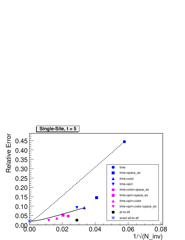
Figure 2: The relative error of the diagonal correlator for a single-site elemental operator (at $t=5$) versus the total number of Dirac matrix inversions required for various dilution schemes with a single stochastic source. Along with these dilution schemes, the point-to-all result and the exact all-to-all result are plotted. The dotted line represents the error falloff expected from increasing the number of time-diluted noise sources. The solid line represents the same for time+color-diluted noise sources.

The horizontal axis in these figures represents $1/\sqrt{N_{inv}}$, where $N_{inv}$ is the total number of required Dirac matrix inversions. In these coordinates, the error falloff due to an increase in the number of noise sources for a fixed dilution scheme will be linear with a flattened approach to the gauge noise limit.

As all the subsequent points in these figures lie well below the dotted line, it is clear that increasing the level of dilution past time dilution is more efficient than adding time-diluted noise sources. However, the improvement is less apparent for the solid line. Here there may be a small gain in the fractional error, but computational cost and storage must be considered. An increase in the number of dilution projectors by a factor $X$ results in an $X^{3}$ increase in the number of components in the source and sink functions of Eq. 2. An increase in the number of diluted noise sources however, results in the same increase to the number of components of the source and sink functions.

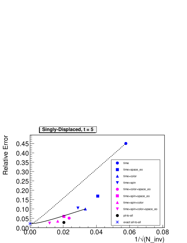
Figure 3: The same as Fig. 2 for a singly-displaced elemental operator.

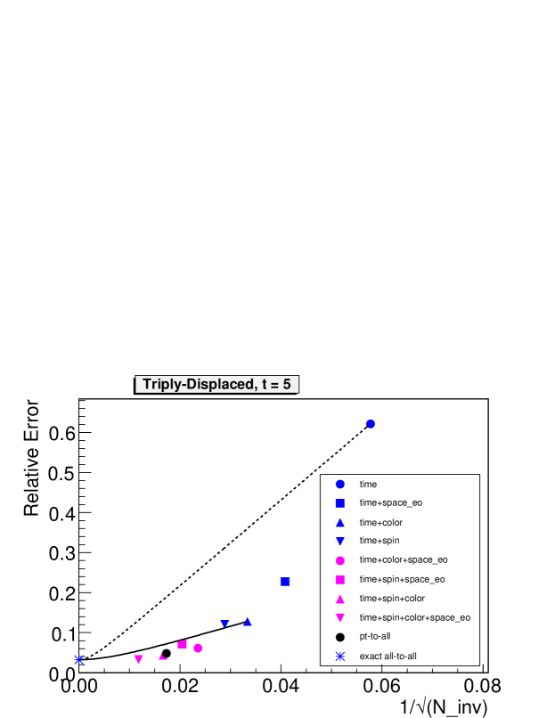
Figure 4: The same as Fig. 2 for a triply-displaced elemental operator. The black point is slightly offset from the pink triangle for clarity.

4 Conclusions

The dilution method for variance reduction has been tested for baryons. As is seen in Figs. 2, 3, and 4, increasing the number of dilution projectors usually results in a decrease in error that is greater than the naive $1/\sqrt{N}$ expected from increasing the number of diluted noise sources. It is also apparent from these figures that time + spin + color dilution possesses comparable error to the point-to-all method and that time + spin + color + spatial even-odd dilution is comparable to the exact all-to-all result.

While it is clear that increasing the level of dilution past time dilution is more efficient than adding more time-diluted sources, it may not be most efficient to employ dilution schemes finer than time + color dilution but rather increase the number of time + color-diluted noise sources. To complete these tests, simple fits to the diagonal correlators must be compared, as well as spatially extended meson operators. A new method [9] is also being explored which will yield exact all-to-all propagators for a comparable cost. This method is based on a spectral decomposition of the quark smearing operator and will retain the desirable property of the factorization of the source and sink functions.

5 Acknowledgments

This work was done with code written using the Chroma software suite [10]. The authors would like to thank Mike Peardon for valuable discussions about dilution methods. This work was supported by the U.S. National Science Foundation under the Award PHY-0653315 and in part by Jefferson Science Associates, LLC under U.S. Dept. of Energy Contract No. DE-AC05-06OR23177.

References

- [1] A. C. Lichtl, PhD Thesis, hep-lat/0609019.
- [2] J. Bulava et al., AIP Conf. Proc. 947, 137 (2007). (arXiv:0708.2145 [hep-lat])
- [3] E. Engelson et al., These Proceedings.
- [4] K. J. Juge et al., These Proceedings.
- [5] R. G. Edwards et al.. PoS LAT2007, 108 (2007). (arXiv:0710.3571 [hep-lat])
- [6] J. Foley et al., Comput. Phys. Commun. 172 (2005) 145.
- [7] S. Basak et al., Phys. Rev. D72 (2005) 094506.
- [8] C. Morningstar and M. Peardon, Phys. Rev. D 69, 054501 (2004).
- [9] M. Peardon, Private Communication.
- [10] R. G. Edwards and B. Joo, Nuc. Phys. B140 (Proc. Suppl.) p832, 2005. (arXiv:hep-lat/0409003)