Constraint satisfaction problems with isolated solutions are hard

Abstract

We study the phase diagram and the algorithmic hardness of the random ‘locked’ constraint satisfaction problems, and compare them to the commonly studied ’non-locked’ problems like satisfiability of boolean formulas or graph coloring. The special property of the locked problems is that clusters of solutions are isolated points. This simplifies significantly the determination of the phase diagram, which makes the locked problems particularly appealing from the mathematical point of view. On the other hand we show empirically that the clustered phase of these problems is extremely hard from the algorithmic point of view: the best known algorithms all fail to find solutions. Our results suggest that the easy/hard transition (for currently known algorithms) in the locked problems coincides with the clustering transition. These should thus be regarded as new benchmarks of really hard constraint satisfaction problems.

I Introduction

Constraint satisfaction problems (CSPs) play a crucial role in theoretical and applied computer science. Their wide range of applicability arises from their very general nature: given a set of $N$ discrete variables subject to $M$ constraints, a CSP consists in deciding whether there exists an assignment of variables which satisfies simultaneously all the constraints. When such an assignment exists we call it a solution and aim at finding it. One of the most important questions about a CSP is how hard it is to find a solution or prove that there is none. Many of the CSPs belong to the class of NP-complete problems Cook (1971); Garey and Johnson (1979). This basically means that, if P$\neq$NP, there is no algorithm able to solve the worst case instances of the problem in a polynomial time. Next to the question of the worst case computational complexity arises the less explored question of typical case complexity. A pivotal step in understanding the typical case complexity is the study of random CSPs where each constraint involves a finite number of variables. Pioneering work on this subject Cheeseman et al. (1991); Mitchell et al. (1992) discovered that many problems are empirically harder close to the so-called satisfiability phase transition. This is a phase transition appearing at a critical constraint density $\alpha_{s}$ such that for $M/N=\alpha<\alpha_{s}$ almost every large instance of the problem has at least one solutions, and for $\alpha>\alpha_{s}$ almost all large instances have no solution.

Studies of phase transitions such as the one occuring in the satisfiability problem are natural for statistical physicists. Indeed the methods developed to study frustrated disordered systems like glasses and spin glasses Mézard et al. (1987) have turned out to be very fruitful in the study of several CSPs. In particular they allow some structural studies which aim at understanding how the difficulty of a problem is related to the geometrical organization of its solutions. Several other phase transitions were described in this context. The most important one is probably the clustering transition Mézard et al. (2002); Biroli et al. (2000), known as the dynamical glass transition in the mean field theory of glasses. It was computed that in the region where the density of constraints is below the satisfiability threshold there exists a phase where the space of solutions splits into ergodically separated groups – clusters. Another important property of the clusters concerns the freezing of the variables. A variable is frozen in a cluster if it takes the same value in all the solutions of this cluster. It has been conjectured that the clustering Mézard and Zecchina (2002) and the freezing of variables Zdeborová and Krzakala (2007) are two ingredients which contribute to make a random CSP hard. But the predictions for the easy/hard transition in a general random CSP are still not fully quantitative. The present work provides further insight into this subject.

In this paper we present a detailed study of the locked CSPs, introduced recently in Zdeborová and Mézard (2008). The special property of the locked problems is that clusters are point-like: every cluster contains only one solution. Therefore, as soon as the system is in a clustered phase, all the variables are frozen in each cluster. The clustering and the freezing phase transitions occur simultaneously. Consequently the organization of the space of solutions is much simpler than in the commonly studied K-satisfiability or graph coloring Mézard et al. (2002); Mulet et al. (2002); Krzakala et al. (2007); Zdeborová and Krzakala (2007); Montanari et al. (2008). But at the same time, and unlike in the K-satisfiability or graph coloring problems, the whole clustered phase is extremely hard for all existing algorithm and the clustering/freezing threshold seems to coincide very precisely with the onset of this hardness.

The interest in the locked problems is thus twofold:

• Locked problems are very simple: As the clusters of solutions are point-like many of the quantities of interest can be computed using simpler tools than in the canonical K-satisfiability problem. This is in particular interesting from the mathematical point of view, because several of their properties become accessible to rigorous proofs. From a broader point of view the locked problems should be useful as simple models of glass forming liquids because their phase diagram can be studied without any need to introduce the complicated scheme of ‘replica symmetry breaking’ Mézard et al. (1987).

• Locked problems are very hard: From the algorithmic point of view the whole clustered phase of the locked problems is extremely hard, none of the known algorithms is able to find solutions efficiently. This suggests to use locked CSPs as hard benchmarks. At the same time one may hope that the performance of some algorithms will be simpler to analyze when they are applied to the locked problems, compared to the general case.

This paper is organized as follows: In section II we define the random occupation problems and the random locked occupation problems (LOPs) on which we will illustrate our main findings. In section III we write the equations needed to describe the phase diagram of the occupation problems, using well known tools from statistical physics and probability theory. In section IV we summarize the basic properties of the phase diagram in general random CSPs and then discuss in detail the situation in the locked problems. We also discuss the class of so-called balanced LOPs which are even simpler from the mathematical point of view. Finally section V shows our findings about algorithmic performance in the occupation problems: empirical data using the best known random CSP solver – belief propagation reinforcement – indicates that the clustering threshold is close to the boundary between the easy and hard regions. We analyze also the non-locked occupation problems for comparison. A short summary of the results and perspectives conclude the paper in section VI.

II Definitions

II.1 Locked occupation problems

We shall study a broad class of problems called ‘occupation problems’. An occupation problem involves $N$ binary variables $s_{i}\in\{0,1\}$ ($s_{i}=0$ is referred to as “site $i$ is empty”, and $s_{i}=1$ is “occupied”) and $M$ constraints, indexed by $b\in\{1,\dots,M\}$. Each constraint $b$ involves $K_{b}$ distinct variables, and is defined by a ‘constraint word’ $A^{b}$ with $K_{b}+1$ bits, which we write as $A^{b}=A_{0}^{b}A_{1}^{b}\dots A_{K_{b}}^{b}$, where $A_{i}^{b}\in\{0,1\}$. We denote by $\partial b$ the indices of all variables involved in the constraint $b$. The constraint $b$ is satisfied if and only if the sum $r=\sum_{i\in\partial b}s_{i}$ of all its variables is such that $A_{r}^{b}=1$. In other words, in order for constraint $b$ to be satisfied, one needs that the number of occupied sites, $r$, in its neighborhood, must be such that $A_{r}^{b}=1$ (this unified notation for the occupation problems was introduced in Mora (2007)).

Definition: An occupation problem is locked if and only if:

• For every constraint $b\in\{1,\dots,M\}$, the vector $A^{b}$ is such that, for all $i=0,\dots,K-1$: $A_{i}^{b}A_{i+1}^{b}=0$ .

• Every variable appears in at least two different constraints.

In this paper, we shall study only ‘constraint-regular’ problems in which all of the constraints are described by the same constraint word: for all $b\in\{1,\dots,M\}$, $K_{b}=K$ and $A^{b}=A$. Furthermore, in order to focus onto difficult cases, we shall only consider the occupation problems where neither the totally empty nor the totally occupied configurations are solution, i.e. we keep to the cases where $A_{0}=A_{K}=0$. It is convenient to use the factor graph description of a problem Kschischang et al. (2001); Mézard and Montanari (2008), where sites and constraints are vertices, and an edge connects a constraint $a$ to a site $i$ whenever $i$ appears in constraint $a$ (see Fig. 1). An instance of a constraint-regular occupation model is fully described by its factor graph (where all constraint vertices have degree $K$) and the $K+1$ component vector $A$. The locked problems are thus characterized by the facts that (i) there are no consecutive ‘1’ in the word $A=A_{0}A_{1}\dots A_{K}$, and (ii) their factor graph has no leaves.

Well-studied examples of occupation problems include:

• Ising anti-ferromagnet: $A=010$

• Odd parity checks (anti-ferromagnetic $K$-spin model, with $K$ even): $A=01010\dots 1010$

• Positive 1-in-K SAT (exact cover): $A=0100\dots 00$ Raymond et al. (2007)

• Perfect matching in $K$-regular graphs: each variable belongs to two constraints and $A=01000\dots 00$ Zdeborová and Mézard (2006)

• Bicoloring (positive NAE-SAT): $A=0111\dots 110$ Achlioptas and Moore (2006); Castellani et al. (2003); Dall’Asta et al. (2008)

• Circuits going through all the points: $A=001000\dots 00$ Marinari and Semerjian (2006)

All these examples, except the bicoloring, are locked on graphs without leaves.

For the occupation problems which have not been studied previously, we will use names derived in the following way: $A=010100$ is the 1-or-3-in-5 SAT, $A=010010$ is the 1-or-4-in-5 SAT, etc.

Figure 1: A factor graph representation of an instance of the 1-or-3-in-5 SAT ($A=010100$). The squares are the constraints. Full/empty circles are occupied/empty sites. The two parts show two examples of satisfying assignments – “solutions” – of this instance. As there are no leaves (each variable belongs to at least two constraints) and $A$ satisfies $A_{i}A_{i+1}=0$ for all $i=0,\dots,4$, this instance is locked.

From the computational complexity point of view, Schaefer’s theorem Schaefer (1978) implies that most of the occupation problems are NP-complete. The exceptions are the parity checks, which amount to linear systems of equations on $GF(2)$, and some of the cases where the variables have degree 2, such as for instance the perfect matching.

The crucial property of the locked occupation problems is that in order to go from one solution to another one must flip at least a closed loop of variables. This property can be used to generalize the definition of a locked problems to a much wider class of constraint satisfaction problems than the occupation problems, and in particular the variables do not need to be binary. Some examples of locked problems which are not occupation problems are the XOR-SAT (p-spin) problem on factor graphs without leaves Mézard et al. (2003), or all the uniquely extensible models Connamacher and Molloy (2004).

II.2 Ensembles of random occupation problems

We shall study some random ensembles of locked occupation problems, in which the factor graph is chosen from some ensemble of random bipartite graphs. We consider constraint-regular occupation problems where each constraint involves $K$ variables, and is characterized by the constraint word $A$. An ensemble is characterized via a probability distribution $Q(l)$. To create an instance of the random occupation problem with $N$ variables, we draw $N$ independent random numbers $l_{i}$ from the distribution $Q(l)$, with the additional constraint that $\sum_{i=1}^{N}l_{i}/K=M$ is an integer. The factor graph that characterizes an instance is then chosen uniformly at random from all the possible graphs with $N$ variables, and $M$ constraints, such that, for all $i=1\dots N$, the variable $i$ is connected to $l_{i}$ constraints.

In this paper we will consider mainly two degree distributions:

• Regular: $Q(l)=\delta_{l,L}$, in which all the variables take part in $L$ clauses.

• Truncated Poissonian:

  $$Q(0)=Q(1)=0\,,\quad\quad Q(l)=\frac{1}{1-(1+c)\,e^{-c}}\frac{e^{-c}c^{l}}{l!}\quad{\rm for}\quad l\geq 2$$ (1)

  where $c\geq 0$. The average “connectivity” (variable degree) is then

  $$\overline{l}=c\,\frac{1-e^{-c}}{1-(1+c)\,e^{-c}}\ .$$ (2)

  In the cavity method one also needs the excess degree distribution $q(l)$, defined as the distribution of the number of neighbors on one side of an edge chosen uniformly at random:

  $$q(0)=0\,,\quad\quad q(l)=\frac{1}{e^{c}-1}\frac{c^{k}}{k!}\,.$$ (3)

We shall be interested in the properties of large instance, i.e. in the ‘thermodynamic limit’ where one sends $N\to\infty$ and $M\to\infty$, keeping $K$ and $Q(l)$ fixed; this results in a fixed density of constraints $M/N=\overline{l}/K$. Our main results are easily generalizable to any degree distribution $Q(l)$ which has a finite second moment. For every such distribution, a typical factor graph is locally tree-like: the shortest loop going through a typical variable has a length which scales as $\log{N}$. The crucial property of the locked occupation problems is that, in order to go from one solution of the problem to another solution, one must flip at least one closed loop of variables. On the random locally tree-like factor graphs this means that at least $\log{N}$ variables need to be changed.

III The solution of random occupation problems

The cavity method Mézard and Parisi (2001) is nowadays the standard tool to compute the phase diagram of random locally tree-like constraint satisfaction problems. Depending on the structure of the space of solutions of the problem, different versions (levels of the replica symmetry breaking) of the method are needed. In this section we state the cavity equations for the occupation problems. For a detailed derivation and discussion of the method see Mézard and Parisi (2001); Mézard and Montanari (2008).

We index the variables by $i,j,k,\dots$ going from $1$ to $N$, and the constraints by $a,b,c,\dots$ going from $1$ to $M$. The energy of the occupation problems then reads

$$H(\{s\})=\sum_{a=1}^{M}\delta_{A_{\sum_{j\in\partial a}s_{j}},0}\,,$$ (4)

In this paper we shall study only the instances where solutions (ground states of zero energy) exist, and we shall focus on the uniform measure over all solutions.

III.1 The replica symmetric solution

Figure 2: Part of the factor graph to illustrate the meaning of indices in the belief propagation equations (5a-5b).

The replica symmetric version of the cavity method is also known under the name belief propagation Pearl (1982); Kschischang et al. (2001); Mézard and Montanari (2008). It exploits the local tree-like property of the factor graph, assuming that correlations decay fast enough. The basic quantities used in this approach are messages. We define $\psi_{s_{i}}^{a\to i}$ as the probability that the constraint $a$ is satisfied, conditioned to the fact that the value of variable $i$ is $s_{i}$. Similarly, $\chi_{s_{j}}^{j\to a}$ is the probability that the variable $j$ takes value $s_{j}$ conditioned to the fact that the constraint $a$ has been removed from the graph. The messages then satisfy the belief propagation (BP) equations

$$\psi_{s_{i}}^{a\to i} = \frac{1}{Z^{a\to i}}\sum_{\{s_{j}\}}\delta_{A_{s_{i}+\sum_{j}s_{j}},1}\prod_{j\in\partial a-i}\chi_{s_{j}}^{j\to a}\,,$$ (5a)

$$\chi_{s_{j}}^{j\to a} = \frac{1}{Z^{j\to a}}\prod_{b\in\partial j-a}\psi_{s_{j}}^{b\to j}\,,$$ (5b)

where $Z^{a\to i}$ and $Z^{j\to a}$ are normalization constants. Fig. 2 shows the corresponding part of the factor graph. The marginal probabilities (“beliefs”) are then expressed as

$$\chi_{s_{i}}^{i}=\frac{1}{Z^{i}}\prod_{a\in\partial i}\psi_{s_{i}}^{a\to i}\,,$$ (6)

The replica symmetric entropy (logarithm of the number of solutions, divided by the system size) then reads

$$s=\frac{1}{N}\sum_{a}\log{(Z^{a})}-\frac{1}{N}\sum_{i}(l_{i}-1)\log{(Z^{i})}\,.$$ (7)

where

$$Z^{a} = \sum_{\{s_{i}\}}\delta_{A_{\sum_{i}s_{i}},1}\prod_{i\in\partial a}\left(\prod_{b\in\partial i-a}\psi_{s_{i}}^{b\to i}\right)\,,$$ (8a)

$$Z^{i} = \prod_{a\in\partial i}\psi_{0}^{a\to i}+\prod_{a\in\partial i}\psi_{1}^{a\to i}\,,$$ (8b)

are the exponentials of the entropy shifts when the node $a$ and its neighbors (resp. the node $i$) is added.

When one considers an ensemble of random graphs, the probability distribution of the messages can be found via the population dynamics technique Mézard and Parisi (2001). Moreover, on the regular graph ensemble or for some of the balanced problems (see Sec. IV.3) the solution is factorized. In the factorized solution the messages $\chi^{i\to a}$, $\psi^{a\to i}$ are independent of the edge $(ia)$ and the replica symmetric solution can thus be found analytically.

For instance in the regular graph ensemble where each variable is present in $L$ constraints the factorized solution is

$$\psi_{0} = \frac{1}{Z^{\rm reg}}\sum_{r=0}^{K-1}\delta_{A_{r},1}{K-1\choose r}\psi_{1}^{(L-1)r}\psi_{0}^{(L-1)(K-1-r)}\ ,$$ (9a)

$$\psi_{1} = \frac{1}{Z^{\rm reg}}\sum_{r=0}^{K-1}\delta_{A_{r+1},1}{K-1\choose r}\psi_{1}^{(L-1)r}\psi_{0}^{(L-1)(K-1-r)}\,,$$ (9b)

where the normalization $Z^{\rm reg}$ is fixed by the condition $\psi_{0}+\psi_{1}=1$. Given the solution $\psi_{0}$, $\psi_{1}$ of (9a-9b), the entropy reads

$$s_{\rm reg}=\frac{L}{K}\log{\left[\sum_{r=0}^{K}\delta_{A_{r},1}{K\choose r}\psi_{1}^{(L-1)r}\psi_{0}^{(L-1)(K-r)}\right]}-(L-1)\log{\left[\psi_{0}^{L}+\psi_{1}^{L}\right]}\,.$$ (10)

III.2 Reconstruction on trees

Treating the locally tree-like random graph as a tree fails if long range correlations are present in the system. More precisely Mézard and Montanari (2006); Krzakala et al. (2007) the replica symmetric assumption is correct if and only if the so-called point-to-set correlations do decay to zero. The decay of these correlations is closely related Mézard and Montanari (2006) to the problem of reconstruction on trees Mossel (2001) which we explain and analyze in this section.

The reconstruction on trees is defined as follows: First construct a tree of $d$ generations having the same connectivity properties as a finite neighborhood of a random variable in the random factor graph. Assign the root a random value, further assign values iteratively on the descendants uniformly at random but in such a way that the constraints are satisfied. Subsequently forget the assignment everywhere but on the leaves of the tree. The reconstruction on the tree is possible if and only if the information left in the values of the leaves about the value of the root does not go to zero as the size of the tree grows, $d\to\infty$. The replica symmetric assumption is correct if and only if the reconstruction is not possible, in other words if there is no correlation between the root (point) and the leaves (set). Typically, when the average connectivity of variables is small the reconstruction is not possible and when the connectivity is large the reconstruction is possible. The threshold connectivity is called the reconstructibility threshold, or the clustering transition. The clustering is then defined as a minimal decomposition of the space of solutions such that within the components (clusters) the point-to-set correlations do decay to zero Krzakala et al. (2007).

It was shown in Mézard and Montanari (2006) that the analysis of the reconstruction on trees is equivalent to the solution of the one-step replica symmetry breaking (1RSB) equations at the value of the Parisi parameter $m=1$ Mézard and Parisi (2001).

Instead of the general form of the 1RSB equations at $m=1$ (see e.g. Zdeborová (2007)), we shall only discuss here a simpler form called the naive reconstruction in Semerjian (2008). In general the naive reconstruction gives only an upper bound on the reconstructibility threshold, but in the locked problems it gives in fact the full information. The naive reconstruction consists in computing the probability that the value of the root is uniquely implied by the leaves (boundary conditions). Here we give the equations only for regular graph ensembles with variables of connectivity $L$, where the factorized replica symmetric solution (9) holds. Define $\mu_{1}$ (resp. $\mu_{0}$) as the probability that a variable which in the broadcasting had value $1$ (resp. $0$) is uniquely determined by the boundary conditions. One has:

$$\mu_{1} = \frac{1}{\psi_{1}Z^{\rm reg}}\sum_{r=0}^{k}\delta_{A_{r+1},1}\delta_{A_{r},0}\,g_{k}(r)\sum_{s=0}^{s_{1}}{r\choose s}\left[1-(1-\mu_{0})^{l}\right]^{k-r}\left[1-(1-\mu_{1})^{l}\right]^{r-s}(1-\mu_{1})^{ls}\,,$$ (11a)

$$\mu_{0} = \frac{1}{\psi_{0}Z^{\rm reg}}\sum_{r=0}^{k}\delta_{A_{r+1},0}\delta_{A_{r},1}\,g_{k}(r)\sum_{s=0}^{s_{0}}{k-r\choose s}\left[1-(1-\mu_{1})^{l}\right]^{r}\left[1-(1-\mu_{0})^{l}\right]^{k-r-s}(1-\mu_{0})^{ls}\,,$$ (11b)

where $l=L-1$, $k=K-1$, and $g_{k}(r)={k\choose r}(\psi_{1})^{lr}(\psi_{0})^{l(k-r)}$ . The indices $s_{1},s_{0}$ in the second sum of both equations are the largest possible but such that $s_{1}\leq r$, $s_{0}\leq K-1-r$, and $\sum_{s=0}^{s_{1}}A_{r-s}=0$, $\sum_{s=0}^{s_{0}}A_{r+1+s}=0$. The values $\psi_{0}$, $\psi_{1}$ are the fixed point of eqs. (9a-9b), and $Z^{\rm reg}$ is the corresponding normalization.

These lengthy equations have in fact a simple meaning. The first sum is over the possible numbers $r$ of occupied variables on the descendants in the broadcasting. The sum over $s$ is over the number of variables which were not implied by at least one constraint but the configuration of implied variables nevertheless implies the outcoming value. The term $1-(1-\mu)^{l}$ is the probability that at least one constraint implies the variable, $(1-\mu)^{l}$ is the probability that none of the constraints implies the variable.

III.3 Survey Propagation

Survey propagation is a special form of the 1RSB equations corresponding to the value of the Parisi parameter $m=0$ Mézard and Zecchina (2002). The main assumption of the 1RSB approach is that the space of solutions splits into clusters (pure states). To each cluster corresponds one fixed point of BP equations. Survey propagation are then iterative equations for the following probabilities (surveys)

$${\rm Prob}(\chi_{1}^{i\to a}=1,\chi_{0}^{i\to a}=0)=p_{1}^{i\to a}, {\rm Prob}(\psi_{1}^{a\to i}=1,\psi_{0}^{a\to i}=0)=q_{1}^{a\to i},$$ (12a)

$${\rm Prob}(\chi_{1}^{i\to a}=0,\chi_{0}^{i\to a}=1)=p_{0}^{i\to a}, {\rm Prob}(\psi_{1}^{a\to i}=0,\psi_{0}^{a\to i}=1)=q_{0}^{a\to i},$$ (12b)

$$p_{*}^{i\to a}=1-p_{1}^{i\to a}-p_{0}^{i\to a}, q_{*}^{a\to i}=1-q_{1}^{a\to i}-q_{0}^{a\to i},$$ (12c)

where $q_{1/0}^{a\to i}$ is probability over clusters that clause $a$ is satisfied only if variable $i$ takes value $1/0$, $q_{*}^{a\to i}$ is then the probability that clause $a$ can be satisfied by both values $1$ and $0$, similarly $p_{1/0}^{i\to a}$ is probability that variable $i$ have to take value $1/0$ if the clause $a$ is not present, $p_{*}^{i\to a}$ is probability that the variable $i$ can take both values $1$ and $0$ when clause $a$ is not present. The survey propagation equations are then written in two steps, first the update of $p$’s knowing $q$’s

$$p_{1}^{j\to a} = \frac{1}{{\cal N}^{j\to a}}\left[\prod_{b\in\partial j-a}(q_{1}^{b\to j}+q_{*}^{b\to j})-\prod_{b\in\partial j-a}q_{*}^{b\to j}\right],$$ (13a)

$$p_{0}^{j\to a} = \frac{1}{{\cal N}^{j\to a}}\left[\prod_{b\in\partial j-a}(q_{0}^{b\to j}+q_{*}^{b\to j})-\prod_{b\in\partial j-a}q_{*}^{b\to j}\right],$$ (13b)

$$p_{*}^{j\to a} = \frac{1}{{\cal N}^{j\to a}}\prod_{b\in\partial j-a}q_{*}^{b\to j},$$ (13c)

second the update of $q$’s knowing $p$’s

$$q_{s}^{a\to i} = \frac{1}{{\cal N}^{a\to i}}\left[\sum_{\{r_{j}\}}C_{s}(\{r_{j}\})\prod_{j\in\partial a-i}p_{r_{j}}^{j\to a}\right]\ .$$ (14a)

Here ${\cal N}^{j\to a}$ and ${\cal N}^{a\to i}$ are normalization constants, the indices $s$ and $r_{j}$ are in $\{1,0,*\}$. The function $C_{1}$/$C_{0}$ (resp. $C_{*}$) takes values $1$ if and only if the incoming set of $\{r_{j}\}$ forces the variable $i$ to be occupied/empty (resp. let the variable $i$ free), in all other cases the $C$’s are zero. More specifically, let us call $n_{1},n_{0},n_{*}$ the number of indices $1,0,*$ in the set $\{r_{j}\}$ then

• $C_{1}=1$ if and only if $A_{n_{1}+n_{*}+1}=1$ and $A_{n_{1}+n}=0$ for all $n=0\dots n_{*}$;

• $C_{0}=1$ if and only if $A_{n_{1}}=1$ and $A_{n_{1}+1+n}=0$ for all $n=0\dots n_{*}$;

• $C_{*}=1$ if and only if there exists $m,n\in\{0\dots n_{*}\}$ such that $A_{n_{1}+n}=A_{n_{1}+m+1}=1$.

III.4 The first and the second moment

In this section we give the formulas for the first and second moment method in general occupation problems. This allows for a direct probabilistic study of the balanced locked occupation problems introduced below in Sec. IV.3.

For a given instance (or factor graph), $G$, define as ${\cal N}_{G}$ the number of solutions. The first moment is the average of ${\cal N}_{G}$ over the graph ensemble, which can also be written as:

$$\langle{\cal N}_{G}\rangle=\sum_{\{\sigma\}}{\rm Prob}\left(\{\sigma\}\,{\rm is}\,{\rm SAT}\right)\,.$$ (15)

The ‘annealed entropy’ is then defined as $s_{\rm ann}\equiv\log{\langle{\cal N}_{G}\rangle}/N$. It is an upper bound on the quenched entropy, $\langle\log{{\cal N}_{G}}\rangle/N$. In order to compute the first moment we divide variables into groups according to their connectivity and in each group we choose a fraction of occupied variables. The number of ways in which this can be done is then multiplied by the probability that such a configuration satisfies simultaneously all the constraints. After some algebra Zdeborová (2007) we obtain the entropy of solutions with a fraction $0\leq t\leq 1$ of occupied variables:

$$s_{\rm ann}(t)=\sum_{l}Q(l)\log{[1+u(t)^{l}]}+\frac{\overline{l}}{K}\log{\Big{[}\sum_{r=0}^{K}\delta_{A_{r},1}{K\choose r}\left(\frac{t}{u(t)}\right)^{r}(1-t)^{K-r}\Big{]}}\,,$$ (16)

where $u(t)$ is the inverse of

$$t=\frac{1}{\overline{l}}\sum_{l}l\,Q(l)\frac{u^{l}}{1+u^{l}}\,.$$ (17)

The annealed entropy is then $s_{\rm ann}={\rm max_{t}}s_{\rm ann}(t)$.

The second moment of the number of solutions is defined as

$$\langle{\cal N}^{2}_{G}\rangle=\sum_{\{\sigma_{1}\},\{\sigma_{2}\}}{\rm Prob}\left(\{\sigma_{1}\}\,{\rm and}\,\{\sigma_{2}\}\,{\rm are}\,{\rm both}\,{\rm SAT}\right)\,.$$ (18)

The second moment entropy is then defined as $s_{\rm 2nd}\equiv\log{\langle{\cal N}^{2}_{G}\rangle}/N$. The Chebyshev’s inequality gives then a lower bound on the satisfiability threshold via

$${\rm Prob}({\cal N}_{G}>0)\geq\frac{\langle{\cal N}_{G}\rangle^{2}}{\langle{\cal N}^{2}_{G}\rangle}\,.$$ (19)

The second moment is computed in a similar manner as in Achlioptas and Moore (2006); Achlioptas et al. (2005). First we fix that in a fraction $t_{x}$ of nodes the variable is occupied in both the solutions $\sigma_{1},\sigma_{2}$ in (18). In a fraction $t_{y}$ the variable is occupied in $\sigma_{1}$ and empty in $\sigma_{2}$ and the other way round for $t_{z}$. We sum over all possible realizations of $0\leq t_{x},t_{y},t_{z}$ such that $\sum_{w=x,y,z}t_{w}\leq 1$. This is multiplied by the probability that the two configurations $\sigma_{1},\sigma_{2}$ both satisfy all the constraints. After some algebra we obtain Zdeborová (2007):

$$s_{\rm 2nd}(t_{x},t_{y},t_{z})=\frac{\overline{l}}{K}\log{p_{A}(t_{x},t_{y},t_{z})}+\sum_{l}Q(l)\log{\left\{1+\sum_{w\in\{x,y,z\}}[u_{w}(t_{x},t_{y},t_{z})]^{l}\right\}}\,,$$ (20)

where $u_{w}(t_{x},t_{y},t_{z})$, $w\in\{x,y,z\}$, are obtained by inverting the three equations:

$$t_{w}=\frac{1}{\overline{l}}\sum_{l}l\,Q(l)\frac{u_{w}^{l}}{1+u_{x}^{l}+u_{y}^{l}+u_{z}^{l}}\,,\quad\quad w=x,y,z\,,$$ (21)

and the function $p_{A}(t_{x},t_{y},t_{z})$ is defined as

$$p_{A}(t_{x},t_{y},t_{z}) = \sum_{r_{1},r_{2}=0}^{K}\delta_{A_{r_{1}}A_{r_{2}},1}\sum_{s=\max{(0,r_{1}+r_{2}-K)}}^{\min{(r_{1},r_{2})}}{K\choose(r_{1}-s)(r_{2}-s)\,s}\left(\frac{t_{x}}{u_{x}(t_{x},t_{y},t_{z})}\right)^{s}$$ (22)

$$\left(\frac{t_{y}}{u_{y}(t_{x},t_{y},t_{z})}\right)^{(r_{1}-s)}\left(\frac{t_{z}}{u_{z}(t_{x},t_{y},t_{z})}\right)^{(r_{2}-s)}(1-t_{x}-t_{y}-t_{z})^{(K-r_{1}-r_{2}+s)}\,.$$

The second moment entropy is the global maximum: $s_{\rm 2nd}={\rm max}_{t_{x},t_{y},t_{z}}s_{\rm 2nd}(t_{x},t_{y},t_{z})$.

For the regular graphs $Q(l)=\delta_{l,L}$ the expressions for both the first and second moment simplify considerably. For the first moment, the inverse of (17) is explicit $u=[t/(1-t)]^{1/L}$ and thus

$$s_{\rm ann\,reg}(t)=\frac{L}{K}\log{\left\{\sum_{r=0}^{K}\delta_{A_{r},1}{K\choose r}\left[t^{r}(1-t)^{K-r}\right]^{\frac{L-1}{L}}\right\}}\,.$$ (23)

For the second moment the function (21) is also explicitly reversible and the second moment entropy for regular graphs reads

$$s_{\rm 2nd,reg}(t_{x},t_{y},t_{z}) = \frac{L}{K}\log\Bigg{\{}\sum_{r_{1},r_{2}=0}^{K}\sum_{s=\max{(0,r_{1}+r_{2}-K)}}^{\min{(r_{1},r_{2})}}\frac{K!\delta_{A_{r_{1}},1}\delta_{A_{r_{2}},1}}{(r_{1}-s)!\,(r_{2}-s)!\,s!\,(K-r_{1}-r_{2}+s)!}$$ (24)

$$\left[t_{x}^{s}t_{y}^{(r_{1}-s)}t_{z}^{(r_{2}-s)}(1-\sum_{w}t_{w})^{(K-r_{1}-r_{2}+s)}\right]^{\frac{L-1}{L}}\Bigg{\}}\,.$$

IV The Phase Diagram

IV.1 Non-locked occupation problems

The phase diagram of the non-locked occupation problems that we have explored is qualitatively similar to the one of K-satisfiability and graph coloring studied recently in detail in Mézard et al. (2002); Mézard and Zecchina (2002); Krzakala et al. (2007); Zdeborová and Krzakala (2007); Montanari et al. (2008). We thus only briefly summarize the main findings in order to be able to appreciate the difference between the locked and the non-locked problems.

As one adds constraints to a typical non-locked problem the space of solutions undergoes several phase transitions. When the density of constraints is very small the replica symmetric solution is correct and most of the solutions lie in one cluster. As the density of constraints is increased, the point-to-set correlations, defined via the reconstruction on trees, no longer decay to zero. This is the clustering transition, at this point the space of solutions splits into exponentially many well separated (energetically or entropically) clusters. But as long as an exponential number of such clusters is needed to cover almost all the solution the observables like entropy, magnetizations, two point correlations, etc. behave as if the replica symmetric solution was still correct. This phase is called the dynamical 1RSB. When the constraint density is further increased the space of solutions undergoes the so-called condensation transition. In the condensed phase only a finite number of clusters is needed to cover an arbitrarily large fraction of solutions. Increasing again the density of constraints, one crosses the satisfiability transition where all the solutions disappear.

We remind at this point that in the non-locked occupation problems, where the sizes of clusters fluctuates, the survey propagation equations are not equivalent to the reconstruction on trees. More technically said the 1RSB solutions at $m=0$ and at $m=1$ are different, for example a non-trivial solution appears at different connectivities.

A second class of important phase transitions in the space of solutions of the non-locked problems concerns the so-called frozen variables, which might be responsible for the onset of algorithmic hardness Zdeborová and Krzakala (2007). A variable is frozen in a cluster if in all the solutions belonging to that cluster it takes the same value. A cluster is frozen if a finite fraction of variables are frozen in that cluster. A solution is frozen if it belongs to a frozen cluster. As the number of constraints is increased the clusters tend to freeze. We define two transition points. The first one, called the rigidity transition Zdeborová and Krzakala (2007), is defined as the point where almost all solutions become frozen. The second one, the freezing transition, is defined as the point where strictly all solutions become frozen.

In the cavity method every cluster is associated with a solution of the BP equations. A frozen variable $i$ is described by a marginal probability (6) which is either equal to $(\chi^{i}_{0},\chi^{i}_{1})=(1,0)$ or to $(\chi^{i}_{0},\chi^{i}_{1})=(0,1)$. The rigidity transition is then computed as the connectivity at which such “frozen beliefs” $\chi$ appear in the dominating clusters. If this transition happens before the condensation transition then it is given by the onset of a nontrivial solution to the naive reconstruction, eq. (11). The rigidity transition was computed for the graph coloring in Zdeborová and Krzakala (2007); Semerjian (2008), in the bicoloring of hyper-graphs Dall’Asta et al. (2008), or the K-SAT in Montanari et al. (2008); Semerjian (2008). The freezing transition was studied with probabilistic methods in K-SAT with large $K$ in Achlioptas and Ricci-Tersenghi (2006) and numerically in 3-SAT in Ardelius and Zdeborová (2008).

IV.2 Locked occupation problems

Point-like clusters — The main property which makes the locked problems special is that every cluster consists of a single configuration and has thus zero internal entropy. One way to show this is realizing that in the locked problems if $\{s_{i}\}$ is a satisfying configuration then

$$\psi^{a\to i}_{s_{i}}=1\,,\quad\psi^{a\to i}_{\neg s_{i}}=0\,,$$ (25a)

$$\chi^{i\to a}_{s_{i}}=1\,,\quad\chi^{i\to a}_{\neg s_{i}}=0$$ (25b)

is a fixed point of BP eqs. (5a-5b). The corresponding entropy is then zero, as $Z^{i}=Z^{a}=1$ for all $i$, $a$. In the derivation of Mézard and Montanari (2008) the fixed points of the belief propagation equations correspond to clusters. Thus in the locked problems every solution may be thought of as a cluster. Such a situation was previously encountered in a few problems Krauth and Mézard (1989); Martin et al. (2004, 2005) and called the frozen 1RSB because all the variables, clusters and solutions are frozen in such a case.

The clustering transition — In terms of the reconstruction on trees the situation in the locked problems is trivial because the boundary conditions on leaves always imply uniquely all the variables in the body of the tree and also the root. However one may ask what happens if the assignment of a small fraction of the variable on leaves is also forgotten – we call this the small noise reconstruction on trees . In the non-locked problems nothing changes. In the locked problems the small noise reconstruction is not equivalent to the reconstruction. At sufficiently small connectivities the small noise reconstruction is not possible, that is if we introduce a small noise in the leaves all the information about the root is lost. In the same spirit: we showed that every solution corresponds to a fixed point of the belief propagation of the type (25), but we did not ask if such a fixed point is stable under small perturbations. If an infinitesimal fraction of messages in (25) is changed, will the iterations (5a-5b) converge back to the unperturbed fixed point or not? Again for sufficiently small connectivity it will not. This leads us back to a definition of the clustering transition which needs to be refined for the locked problems.

We thus define the clustering transition as the threshold for the small noise reconstruction. As all the clusters are frozen the reconstruction problem is equivalent to the naive reconstruction which deals only with the frozen variables. So for example on the ensemble of random regular graphs it is sufficient to investigate the stability of the solution $\mu_{0}=\mu_{1}=1$ of eqs. (11a-11b) under iteration. It is immediate to see that if $L\geq 3$ then the solution $\mu_{1}=\mu_{0}=1$ of (11a-11b) is always iteratively stable. When $L=2$ we observed empirically that the solution $\mu_{1}=\mu_{0}=1$ is not stable and the only other solutions is $\mu_{1}=\mu_{0}=0$. Thus in the regular graphs ensemble of the locked problems the clustering transition is at $L=3$.

For a general graph ensemble it is simpler to realize that as the internal entropy of clusters is zero the 1RSB solution does not depend on the value of the Parisi parameter $m$. Thus in particular the small noise reconstruction is equivalent to the iterative stability of the BP-like fixed point of the survey propagation equations.

We have found that, in the locked occupation problems, the SP equations (13-14), when initialized randomly, have two possible iterative fixed points:

• The trivial one: $q^{a\to i}_{*}=p^{i\to a}_{*}=1$, $q^{a\to i}_{1}=p^{i\to a}_{1}=q^{a\to i}_{0}=p^{i\to a}_{0}=0$ for all edges $(ai)$.

• The BP-like one: $q^{a\to i}_{*}=p^{i\to a}_{*}=0$, $q^{a\to i}=\psi^{a\to i}$, $p^{i\to a}=\chi^{i\to a}$ for all edges $(ai)$, where $\psi$ and $\chi$ is the solution of the BP equations (5a-5b) found with high probability by iterating the equations from a uniformly random initial condition.

The small noise reconstruction is then investigated, using the population dynamics, from the stability of the BP-like fixed point under iteration. If it is stable then the small noise reconstruction is possible and the phase is clustered. If it is not stable then we are in the liquid phase. From a geometric point of view, we conjecture that in the liquid phase the Hamming distance separation between solutions grows only proportionally to $\log N$; on the contrary, when small noise reconstruction is possible we expect this Hamming distance to be extensive (proportional to $N$).

The satisfiability threshold — The BP eqs. (5a-5b) have many fixed points. However, when we solve them iteratively starting from a random initial condition we always find the same fixed point which does not correspond to a satisfying assignment (25). We call this fixed point and its corresponding entropy the replica symmetric solution. It should actually be thought of as a fixed point of the survey propagation equations as explained in the previous paragraph. The important fact is that it gives the correct entropy (7), and also the correct marginal probabilities.

The satisfiable threshold in the locked problems is then computed as the average connectivity $l_{s}$ at which the replica symmetric entropy (7) decreases to zero Krauth and Mézard (1989), $s(l_{s})=0$. This is the first of many quantities in the locked problems which can be computed with much smaller effort then in the non-locked problems. The condensed phase, where the space of solutions is dominated by a finite number of clusters does not exist in the locked problems, and the condensation transition coincides with the satisfiability threshold.

Figure 3: Sketch of the phase diagram in the locked problems. At low constraint density $\overline{l}<l_{d}$ the solutions are separated by logarithmical distance but if any sort of noise is introduced this separation disappears. In the clustered phase $l_{d}\leq\overline{l}<l_{s}$ the space of solutions is made of well separated single solutions. And eventually the satisfiability transition $l_{s}$ comes beyond which solutions do not exist.

Summary of the phase diagram — In contrast to the zoo of phase transitions in non-locked problems, in the locked problems we find only three phases, sketched in Fig. 3, the critical connectivity values are given in Table 1.

• The liquid phase, for connectivities $\overline{l}<l_{d}$: In this phase the small noise reconstruction is not possible. Equivalently the BP-like iterative fixed point of the survey propagation equations is not stable. If one considers the problem at a very small temperature, the 1RSB equations have only the trivial solution, such a situation was observed previously in the perfect matching problem Zdeborová and Mézard (2006); Zhou and Ou-Yang (2003). We expect that the Hamming distance separation between solutions in this phase is only logarithmic.

• The clustered phase, for $l_{d}<\overline{l}<l_{s}$: In this phase the small noise reconstruction is possible. The BP-like iterative fixed point of the survey propagation equations is stable. The 1RSB equations have a non-trivial solution even at an infinitesimal temperature. We expect that the solutions are separated by an extensive Hamming distance, in other words there is a gap in the weight enumerator function, just like in the XOR-SAT Mora and Mézard (2006). This property is crucial in low density parity check codes Di et al. (2006).

• The unsatisfiable phase, for $\overline{l}>l_{s}$: no more solutions exist.

All the other phase transitions we described for the non-locked problems have become very simple: The clustering transition coincides with the rigidity and freezing. And the satisfiability transition coincides with the condensation one.

A	name	$L_{s}$	$c_{d}$	$c_{s}$	$l_{d}$	$l_{s}$
0100	1-in-3 SAT	3	0.685(3)	0.946(4)	2.256(3)	2.368(4)
01000	1-in-4 SAT	3	1.108(3)	1.541(4)	2.442(3)	2.657(4)
00100*	2-in-4 SAT	3	1.256	1.853	2.513	2.827
01010*	4-odd-PC	5	1.904	3.594	2.856	4
010000	1-in-5 SAT	3	1.419(3)	1.982(6)	2.594(3)	2.901(6)
001000	2-in-5 SAT	4	1.604(3)	2.439(6)	2.690(3)	3.180(6)
010100	1-or-3-in-5 SAT	5	2.261(3)	4.482(6)	3.068(3)	4.724(6)
010010	1-or-4-in-5 SAT	4	1.035(3)	2.399(6)	2.408(3)	3.155(6)
0100000	1-in-6 SAT	3	1.666(3)	2.332(4)	2.723(3)	3.113(4)
0101000	1-or-3-in-6 SAT	6	2.519(3)	5.123(6)	3.232(3)	5.285(6)
0100100	1-or-4-in-6 SAT	4	1.646(3)	3.366(6)	2.712(3)	3.827(6)
0100010	1-or-5-in-6 SAT	4	1.594(3)	2.404(6)	2.685(3)	3.158(6)
0010000	2-in-6 SAT	4	1.868(3)	2.885(4)	2.835(3)	3.479(4)
0010100*	2-or-4-in-6 SAT	6	2.561	5.349	3.260	5.489
0001000*	3-in-6 SAT	4	1.904	3.023	2.856	3.576
0101010*	6-odd-PC	7	2.660	5.903	3.325	6

Table 1: The locked cases of the occupation CSPs for $K\leq 6$. In the regular graphs ensemble the space of solutions is clustered for $L\geq L_{d}=3$, and the problem is unsatisfiable for $L\geq L_{s}$. The values $c_{d}$ and $c_{s}$ are the critical parameters of the truncated Poissonian ensemble (1), the corresponding average connectivities $l_{d}$ and $l_{s}$ are given via eq. (2). In all there problems the replica symmetric solution is stable at least up to the satisfiability threshold. The balanced cases are marked as *, their dynamical threshold follows from (29), and their satisfiability threshold can be computed from the second moment method.

Finally we would like to mention the stability of the frozen 1RSB solution towards more levels of replica symmetry breaking. In more geometrical terms, one should check whether the solutions do not tend to aggregate into clusters. This is called stability of type I in the literature Montanari and Ricci-Tersenghi (2003); Rivoire et al. (2004); Krzakala and Zdeborová (2008). In the locked problems it is equivalent to the finiteness of the spin glass susceptibility. In all the locked occupation problems we have studied, including all those in Tab. 1, we have seen that the frozen 1RSB solution is always stable in the satisfiable phase and sometimes becomes unstable at a point in the unsatisfiable phase. This means that our description of the satisfiable phase, and the determination of the thresholds $l_{d}$ and $l_{s}$, should be exact.

IV.3 The balanced LOPs

We have seen that the phase diagram in the locked problems is much simpler than in the more studied constraint satisfaction problems as the K-SAT or coloring. In this section we describe a subclass of the locked problems — the so-called balanced locked problems — where the situation is even simpler. In particular, the clustering and the satisfiability threshold can be determined easily, and the second moment method can be used to prove rigorously the validity of this determination of the satisfiability threshold. This makes the balanced locked problems very interesting from the mathematical point of view.

The balanced occupation problems are defined via the property that two random solutions are almost surely at Hamming distance $N/2+o(N)$. This property may of course depend on the connectivity distribution $Q(l)$. A necessary condition for the problem to be balanced it that the vector $A$ be palindromic, meaning that $A_{r}=A_{K-r}$. But not all the palindromic problems are balanced, the simplest such example is the 1-or-4-in-5 SAT, $A=010010$, where the symmetry is spontaneously broken in the same way as in a ferromagnetic Ising model.

As we argued in the previous section in the locked problems the replica symmetric approach (BP) gives the exact marginal probabilities and total entropy. Therefore a problem is balanced if and only if the iterative fixed point of the BP equations (5a-5b) is such that all the beliefs are equal to $1/2$.

We do not know of any simpler general rule to decide if a problem is balanced. For $K\leq 12$, there is no exception to the following empirical rule: all the problems which can be obtained from a Fibonacci-like recursion

$$0A_{K}0=A_{K+2}\quad\quad 01A_{K}10=A_{K+4}$$ (26)

from $A_{2}=010$ or $A_{4}=01010$ are balanced in their satisfiable phase. There are, however, other balanced locked problems which cannot be obtained this way, the simplest example is $A=0001001000$.

Clustering threshold in the balanced LOPs: The clustering threshold is given by the small noise reconstruction, i.e. by the stability of the naive reconstruction procedure as explained in Sec. IV.2. In balanced LOPs, the messages are symmetric, $\psi_{0}=\psi_{1}=1/2$, and thus also the probability for the root variable to be uniquely determined by the leaves is independent of the value which has been broadcast: $\mu_{0}=\mu_{1}=\mu$. For a graph ensemble with excess degree distribution $q(l)$, one can write explicitly the self-consistency condition on $\mu$:

$$\mu=\frac{2}{g_{A}}\sum_{r=0}^{k}\delta_{A_{r+1},1}\delta_{A_{r},0}{k\choose r}\sum_{s=0}^{s_{1}}{r\choose s}\left[1-\sum_{l=0}^{\infty}q(l)(1-\mu)^{l}\right]^{k-s}\left[\sum_{l=0}^{\infty}q(l)(1-\mu)^{l}\right]^{s}\,,$$ (27)

where $k=K-1$, and $g_{A}=\sum_{r=0}^{k}\delta_{A_{r+1},1}{k\choose r}+\sum_{r=0}^{k}\delta_{A_{r},1}{k\choose r}$. For the ensemble of graphs with truncated Poissonian degree distribution of coefficient $c$ we derive from (3)

$$\mu=\frac{2}{g_{A}}\sum_{r=0}^{k}\delta_{A_{r+1},1}\delta_{A_{r},0}{k\choose r}\sum_{s=0}^{s_{1}}{r\choose s}\left(\frac{1-e^{-c\mu}}{1-e^{-c}}\right)^{k-s}\left(\frac{e^{-c\mu}-e^{-c}}{1-e^{-c}}\right)^{s}\,.$$ (28)

The clustering threshold is defined as the value of $c$ where the fixed point $\mu=1$ becomes unstable. One gets:

$$\frac{e^{c_{d}}-1}{c_{d}}=K-1-\frac{\sum_{r=0}^{K-2}\delta_{A_{r+1,1}}\,\delta_{A_{r-1},0}\,\delta_{A_{r},0}\,{K-1\choose r}}{\sum_{r=0}^{K-2}\delta_{A_{r+1},1}\,{K-1\choose r}}\,.$$ (29)

These values are summarized in Table 1, where the balanced locked problems are marked by a $\ast$.

Satisfiability threshold in the balanced LOPs: For the balanced locked problems the replica symmetric entropy is given by:

$$s_{\rm sym}(\overline{l})=\log{2}+\frac{\overline{l}}{K}\log{\left[2^{-K}\sum_{r=0}^{K}\delta_{A_{r},1}{K\choose r}\right]}\,,$$ (30)

where $\overline{l}$ is the average degree of variables. Notice the simple form of this entropy: in the balanced locked problems each added constraint destroys a fraction of solutions exactly equal to the fraction of configurations that satisfy a single constraint. The satisfiability threshold is then given by the point $l_{s}$ where this entropy is zero.

Second moment method in the balanced LOPs: In all the balanced LOPs that we have considered we found numerically that the second moment entropy, (20), is exactly twice the annealed entropy (16), $2s_{\rm ann}=s_{\rm 2nd}$. A hint that this may happen comes from the following observations:

• The annealed entropy (16) has a stationary point at $t=1/2$ ($u=1$, $x=1$). At this stationary the entropy evaluates to (30).

• The second moment entropy (20) has a stationary point at $t_{x}=t_{y}=t_{z}=1/4$ ($u_{x}=u_{y}=u_{z}=1$, $x=y=z=1$). At this stationary point the second moment entropy evaluates to twice the annealed entropy (30). This can be seen using the Vandermonde’s combinatorial identity

  $${K\choose r_{2}}=\sum_{s=0}^{r_{1}}{r_{1}\choose s}{K-r_{1}\choose r_{2}-s}\,.$$ (31)

We checked numerically that in the balanced LOPs the global maxima of $s_{\rm ann}$ and $s_{\rm 2nd}$ is always given by these stationary points (the second moment entropy has another stationary point at $t_{x}=1/2,t_{y}=t_{z}=0$ or $t_{x}=0,t_{y}=t_{z}=1/2$, but at this point it is equal to the first moment entropy at $t=1/2$). On the contrary, in the non-locked or non-balanced problems we always found another competing maximum.

If one accepted the result $2s_{\rm ann}=s_{\rm 2nd}$, and made the reasonable assumption that the satisfiability threshold is sharp, then Chebyshev’s inequality (19) would prove the correctness of the satisfiability threshold computed from (30). Therefore the full class of balanced LOPs is a candidate for a rigorous mathematical determination of the satisfiability threshold. This would be quite interesting, as it would noticeably enlarge the list of problems where the threshold is known rigorously (so far only a handful of sparse NP-complete CSPs are in this category : the 1-in-$K$ SAT Achlioptas et al. (2001a); Raymond et al. (2007), the $2+p$-SAT Cocco et al. (2003); Achlioptas et al. (2001b) and the $(3,4)$-UE-CSP Connamacher and Molloy (2004)).

Let us summarize qualitatively what are the main features of the balanced locked occupation problems that make the fluctuations of the number of solutions so small that the second moment method presumably gives the exact satisfiability threshold.

• Balancing — It is well known that the second moment method works better if most of the weight is on the most numerous configurations (that is the half-filling ones). In the K-SAT problem several reweighting schemes were introduced in order to improve the second moment lower bounds Achlioptas and Moore (2006); Achlioptas et al. (2005). This is also the reason why the second moment bound is much sharper in the balanced NAE-SAT (bicoloring) than in the K-SAT Achlioptas and Moore (2006).

• Reducing fluctuations in the connectivity — Naturally, reducing the fluctuations of the variables connectivity reduces the fluctuation of the number of solutions. Our work shows that the necessary step is not to have leaves. Fluctuating higher degrees do not really pose a problem.

• Locked nature of the problem — And finally the key point is the locked structure of the problem. It was remarked in Ardelius and Zdeborová (2008) that the clusters-related quantities fluctuate much less than the solutions-related ones. Thus the fact that clusters do not have a fluctuating size, but size $1$ is the crucial property needed to make the second moment method sharp. This is exactly what happens in the XOR-SAT problem, where the second moment becomes exact when it is restricted to the ’core’ of the graph Mézard et al. (2003); Cocco et al. (2003)

V Numerical studies

We shall show in this section that the LOPs, in their whole clustered phase, seem to be very hard from the algorithmic point of view. We shall illustrate this by testing and analyzing the performance of some of the best algorithms developed for random 3-satisfiability, the canonical hard constraint satisfaction problem.

Our first study uses a complete algorithm and shows that, like in other problems such as satisfiability and coloring, the hardest instances are found in the neighborhood of the satisfiability transition. We then turn to incomplete algorithms, which are aimed at finding a SAT configuration when it exists.

The best performance for incomplete algorithms is nowadays attributed to the survey propagation inspired decimation Mézard and Zecchina (2002); Parisi (2003) and the survey propagation inspired reinforcement Chavas et al. (2005). In the random 3-SAT problem both of these algorithms were reported to work in linear time (or at most log-linear time) up to a constraint density about $\alpha=4.252$, to be compared with the satisfiability threshold $\alpha_{s}=4.267$ and the clustering transition $\alpha_{d}=3.86$.

As we saw in Sec. IV.2, in the LOPs, the survey propagation algorithm has no advantage over the belief propagation algorithm. We thus study the performance of the BP inspired decimation and reinforcement. The conclusions are as follows: the BP decimation fails in the LOPs even at very low connectivities; the BP reinforcement works in linear time in the non-clustered phase but fails in the clustered phase.

V.1 Exhaustive search results

One way to solve a LOP is to transform it into a conjunctive normal form (CNF), and use some of the open source complete solvers of the satisfiability problem. We have done such a study for the 1-or-3-in-5 SAT problem. We have generated random instances of this problem from a truncated Poisson ensemble, with $M$ constraints. Each instance has been transformed into a satisfiability formula by mapping every constraint into $\sum_{r=0}^{K}\delta_{A_{r},0}{K\choose r}$ CNF clauses: for every constraint of $K$ variables, one creates as many CNF clauses, out of the $2^{K}$ possible clauses, as there are forbidden configurations. We have applied a branch-and-bound based open-source SAT solver called MiniSat 1.14 Eén and Sorensson (2004) to test the satisfiability and to compute the running time needed by this algorithm to decide the satisfiability.

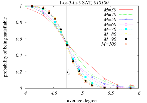
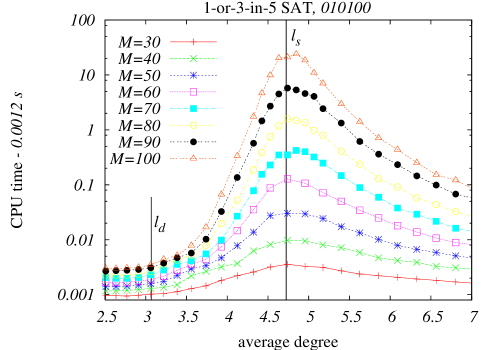
Figure 4: Left: Probability that a random instance of the 1-or-2-in-5 SAT is satisfiable, versus the average degree. The probability is computed from $500$ instances generated from the truncated Poisson ensemble. The vertical line shows the analytical prediction of the value of the satisfiability transition. Right: Median over the same $500$ instances of the CPU running time of the complete algorithm MiniSat 1.14 (we have subtracted $0.0012$ seconds from the CPU time, as this is approximately where is extrapolates for small average degree and zero system size). Alternatively one could plot the number of backtracking steps, which has a qualitatively identical behavior.

Figure 4, left, shows the probability that an instance is satisfiable, plotted versus the average degree. It displays the typical behavior of a phase transition rounded by finite size effects. Figure 4, right, shows the median value of the CPU time which was used to solve an instance of the decision problem on a 2GHz MacBook laptop (note the logarithmic scale), plotted versus the average degree. The hardest instances appear around the satisfiability threshold $l_{s}$, and the time needed by the algorithm in this region clearly grows exponentially with the size. Hard satisfiable instances start to appear around $\overline{l}\simeq l_{d}$, although it is difficult to assert from this data where the exponential behavior really starts. For larger system sizes it seems that the exponential behaviour starts way below the dynamical threshold $l_{d}$.

The data shows the same qualitative behavior as has been found in similar studies of satisfiability, with the difference that the relative width, $(l_{s}-l_{d})/l_{s}$, of the clustered phase is larger in this case than it is in the $K=3$ or $K=4$ satisfiability problems. The existence of LOPs with such a broad clustered phase is an appealing feature for numerical studies. In the following sections of this paper we argue that in the locked problems the easy-hard algorithmic threshold for the best-known incomplete solvers coincides with the clustering transition $l_{d}$.

V.2 Decimation fails in LOPs

In BP inspired decimation one uses the knowledge of the marginal probabilities estimated from BP in order to identify the most biased variable, fix it to its most probable value, and reduce the problem. Such an algorithm usually works well even in the clustered region (for performance in K-SAT and coloring see Krzakala et al. (2007); Zdeborová and Krzakala (2007)). In the locked occupation problems the BP decimation fails badly. For example in the 1-or-3-in-5 SAT problem, on the truncated Poisson graphs with $M=2\cdot 10^{4}$ constraints, the probability of success is about 25% at $\overline{l}=2$, and less than 5% at $\overline{l}=2.3$, way below the clustering threshold $l_{d}\simeq 3.07$. Interestingly, the precursors of the failure of the BP decimation algorithm observed for instance in graph coloring are not present in the locked problems. In particular the BP equations converge during all the process and the normalizations in the BP equations (5a-5b) stay finite.

Although we do not know how to analyze directly the BP decimation process, the mechanisms explaining the failure of the decimation strategy can be understood using the approach of Montanari et al. (2007). The idea is to analyze an idealized decimation process, where the variable to be fixed is chosen uniformly at random and its value is chosen according to its exact marginal probability. If its value is chosen according to the BP marginal we speak about the uniform BP decimation. If BP would give a fair approximation to the exact marginal throughout the decimation process, the uniform BP decimation should be equivalent to the ideal decimation. In the ideal decimation, the reduced problem obtained after $\theta N$ steps is statistically equivalent to the reduced problem created by choosing a solution uniformly at random and revealing a fraction $\theta$ of its variables, which we now analyze, following the lines of Montanari et al. (2007).

Given an instance of the CSP, consider a solution taken uniformly at random and reveal the value of each variable with probability $\theta$. Denote $\Phi$ the fraction of variables which either have been revealed or are directly implied by the revealed ones. We can compute $\Phi(\theta)$ using the replica symmetric cavity method (which is correct in the satisfiable phase of locked problems) as follows.

Denote by $\phi^{i\to b}_{s}$ the probability that a variable $i$ is implied conditioned on the value $s$ of the variable $i$ and on the absence of the edge $(ib)$; denote by $q_{s}^{a\to i}$ the probability that constraint $a$ implies variable $i$ to be $s$ conditioned on: (1) variable $i$ takes the value $s$ in the solution we chose, (2) variable $i$ was not revealed directly and (3) the edge $(ai)$ is absent. Then $\phi^{i\to b}_{s}$ is given by:

$$\phi^{i\to b}_{s}=\theta+(1-\theta)\left[1-\prod_{a\in\partial i-b}(1-q_{s}^{a\to i})\right]\,,$$ (32)

meaning that the variable $i$ was either revealed or not, and if not it is implied if at least one of the incoming constraints implies it. We shall write the expression for $q_{s}^{a\to i}$ only for occupation problems on random regular graphs where the replica symmetric equation is factorized. Then $q_{s}^{a\to i}$ and $\phi^{i\to b}_{s}$ are independent of $a,b,i$: $q_{s}^{a\to i}=q_{s}$ and $\phi^{i\to b}_{s}=\phi_{s}$. The conditional probability $q_{s}$ is the ratio of the probability that variable $i$ takes the value $s$ and is implied by the constraint $a$ on one hand, and the probability that variable $i$ takes the value $s$ on the other hand:

$$q_{1} = \frac{1}{\psi_{1}Z^{\rm reg}}\sum_{r=0}^{k}\delta_{A_{r},0}\delta_{A_{r+1},1}{k\choose r}(\psi_{1})^{lr}(\psi_{0})^{l(k-r)}\sum_{s=0}^{s_{1}}{r\choose s}\phi_{0}^{k-r}\phi_{1}^{r-s}(1-\phi_{1})^{s}\,,$$ (33a)

$$q_{0} = \frac{1}{\psi_{0}Z^{\rm reg}}\sum_{r=0}^{k}\delta_{A_{r},1}\delta_{A_{r+1},0}{k\choose r}(\psi_{1})^{lr}(\psi_{0})^{l(k-r)}\sum_{s=0}^{s_{0}}{k-r\choose s}\phi_{1}^{r}\phi_{0}^{k-r-s}(1-\phi_{0})^{s}\,,$$ (33b)

where $l=L-1$, $k=K-1$. The sum over $r$ goes over all the possible numbers of $1$’s being assigned on the incoming variables, and the numbers $\psi_{0},\psi_{1}$ are the cavity probabilities, solutions of the BP equations (9a-9b). The indices $s_{1},s_{0}$ in the second sum of both equations are the largest possible but such that $s_{1}\leq r$, $s_{0}\leq K-1-r$, and $\sum_{s=0}^{s_{1}}A_{r-s}=0$, $\sum_{s=0}^{s_{0}}A_{r+1+s}=0$. The terms $\phi^{k-r}_{0}\phi^{r-s}_{1}(1-\phi_{1})^{s}$ and $\phi^{r}_{1}\phi^{k-r-s}_{0}(1-\phi_{0})^{s}$ are the probabilities that a sufficient number of incoming variables was revealed such that the out-coming variable is implied (not conditioned on its value). $Z^{\rm reg}$ is the normalization in (9a-9b).

Iterations of eqs. (32-33) with the initial condition $\phi=\theta$ give us the fixed point for $q_{0},q_{1}$. The total probability that a variable is fixed is then computed as

$$\Phi(\theta)=\theta+(1-\theta)\left\{\mu_{1}[1-(1-q_{1})^{L}]+\mu_{0}[1-(1-q_{0})^{L}]\right\}\,,$$ (34)

where $\mu_{0},\mu_{1}$ are the total BP marginals, $\mu_{s}=\psi_{s}^{L}/(\psi^{L}_{0}+\psi^{L}_{1})$. Notice the analogy between eqs. (33b-33a) and the equations for the naive reconstruction (11b-11a).

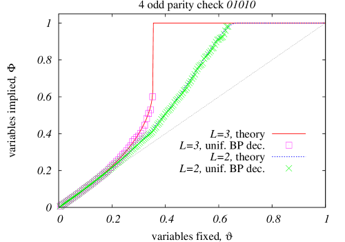
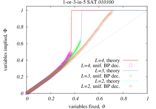
Figure 5: Analytical and numerical study of the BP inspired uniform decimation. The number of variables which are directly implied, $\Phi(\theta)$, is plotted against the number of fixed variables $\theta$ in two of the LOPs on the regular graph ensemble with connectivity $L$.

In Fig. 5 we compare the function $\Phi(\theta)$ obtained from the analytical study of ideal decimation (34) with the experimental performance of the uniform BP decimation. Before the failure of the decimation algorithm (when a contradiction is encountered) the two curves are in very good agreement. This study shows two different reasons for the failure of the algorithm:

• Avalanche of direct implications – In some cases the function $\Phi(\theta)$ has a discontinuity at a certain spinodal point $\theta_{s}$ (e.g. $\theta_{s}\approx 0.46$ at $L=3$ for the 1-or-3-in-5 SAT problem). For $\theta<\theta_{s}$, fixing one variable generates a finite number of direct implications. As the loops are of order $\log{N}$ these implications never lead to a contradiction. At the spinodal point $\theta_{s}$, fixing one more variable generates an extensive avalanche of direct implications. Small (order $1/N$) errors in the previously used BP marginals may thus lead to a contradiction. This indeed happens in almost all the runs we have done. For more detailed discussion see Montanari et al. (2007).

• No more free variables – The second reason for the failure is specific to the locked problems, more precisely to the problems where $\phi_{0}=\phi_{1}=1$ is a solution of eqs. (32-33). In these cases it may happen that the function $\Phi(\theta)\to 1$ at some $\theta_{1}<1$ (e.g. $\theta_{1}\approx 0.73$ at $L=4$ for the 1-or-3-in-5 SAT problem). In other words if we reveal a fraction $\theta>\theta_{1}$ of variables from a random solution, the reduced problem will be compatible with only that given solution. Again, if there has been a little error in the previously fixed variables, the BP uniform decimation ends up in a contradiction. If on the contrary the function $\Phi(\theta)$ reaches the value 1 only for $\theta=1$ then the residual entropy is positive and there might be at each step some space to correct previous small errors, demonstrated on a non-locked problem in Fig. 6.

These two reasons of failure of the BP uniform decimation seem to be of quite different nature. But they have one property in common. As the point of failure is approached we observe that almost all the variables which are being fixed were already implied. The same sign of failure can be observed also in the maximal BP decimation. In Fig. 6 we compare the two procedures. On the $x$-axes we plot the number of variables which could have taken both the values just before they were fixed. On the $y$-axes the number of variables which could take only one value before they were fixed plus the number of implied variables. The failure of both the versions of the BP decimation algorithms is then related to the divergence of the derivative of the function $y(x)$.

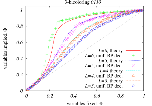
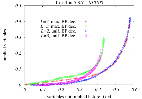
Figure 6: Left: For comparison, the BP uniform decimation works well on the non-locked problems, the example is for bicoloring. Right: Comparison of the uniform BP decimation with the maximal BP decimation. The number of variables which are directly implied or were directly implied before being fixed is plotted against the number of variables which were free just before being fixed. The behavior of the two decimation strategies is similar. The divergence of the derivative of this function marks the point of failure.

V.3 The BP reinforcement algorithm

BP reinforcement is currently the most efficient way of using the BP equations in a solver. It was originally introduced in Chavas et al. (2005), and has also been used in Braunstein and Zecchina (2006); Dall’Asta et al. (2008). The main idea is to add an ‘external bias’ $\mu_{s_{i}}^{i}$ which biases the variable $i$ in the direction of the marginal probability computed from the BP messages. This modifies BP eq. (5b) to

$$\psi_{s_{i}}^{a\to i} = \frac{1}{Z^{a\to i}}\sum_{\{s_{j}\}}\delta_{A_{s_{i}+\sum_{j}s_{j}},1}\prod_{j\in\partial a-i}\chi_{s_{j}}^{j\to a}\,,$$ (35a)

$$\chi_{s_{i}}^{i\to a} = \frac{1}{Z^{i\to a}}\,\mu^{i}_{s_{i}}\prod_{b\in\partial i-a}\psi_{s_{i}}^{b\to i}\,,$$ (35b)

We remind that the belief on variable $i$ (the BP estimate of its marginal) $\chi_{s_{i}}^{i}$, without taking into account the bias $\mu$, is given by eq. (6).

We tried several implementations of how the external bias $\mu_{s_{i}}^{i}$ is updated and found the best performance for the following one

$$\mu^{i}_{1}=\pi,\quad\mu^{i}_{0}=1-\pi,\quad{\rm if}\quad\chi^{i}_{0}>\chi^{i}_{1}\,,$$ (36a)

$$\mu^{i}_{1}=1-\pi,\quad\mu^{i}_{0}=\pi,\quad{\rm if}\quad\chi^{i}_{0}\leq\chi^{i}_{1}\,,$$ (36b)

where $0\leq\pi\leq 1/2$ is a parameter which needs to be optimized. In the iterative update of the BP reinforcement, the external bias is not updated at every BP iteration, but only with probability

$$p(t)=1-(1+t)^{-\gamma}\,.$$ (37)

where $t$ is the time step, and $\gamma$ a parameter to be optimized. The pseudocode of the algorithm is then as follows.

• $\textnormal{BP-Reinforcement}(T,\gamma,\pi)$
     1Initialize $\mu^{i}_{s_{i}}$ and $\psi_{s_{i}}^{a\to i}$ randomly; 2$t\leftarrow 0$; 3Compute the current configuration $r_{i}={\rm argmax}_{s_{i}}\mu^{i}_{s_{i}}$; 4repeat Make one sweep of the BP iterations (35a-35b); 5 update every bias $\mu_{s_{i}}^{i}$ with probability $p(T)$ according to (36a-36b); 6 Update $r_{i}={\rm argmax}_{s_{i}}\mu^{i}_{s_{i}}$; 7 $t\leftarrow t+1$; 8 until$\{r\}$ is a solution or $t>T$;

This algorithm depends on two empirical parameters, $\gamma$ and $\mu$. We generally use $\gamma=0.1$. The optimization of the bias strength $\pi$ is crucial. Empirically we observed three different regimes:

• $\pi_{\rm BP-like}<\pi<0.5$: When the bias is weak, BP-Reinforcement converges very fast to a BP-like fixed point, the values of the local fields do not point towards any solution. On contrary many constraints are violated by the final configuration $\{r_{i}\}$.

• $\pi_{\rm conv}<\pi<\pi_{\rm BP-like}$: BP-Reinforcement converges to a solution $\{r_{i}\}$.

• $0<\pi<\pi_{\rm conv}$: When the bias is too strong, BP-Reinforcement does not converge. And many constraints are violated by the configuration $\{r_{i}\}$ which is reached after $T_{\rm max}$ steps.

When the constraint density in the CSP is large the regime (b) disappears and $\pi_{\rm conv}=\pi_{\rm BP-like}$. Clearly, the goal is to find $\pi_{\rm conv}<\pi<\pi_{\rm BP-like}$. The point $\pi_{\rm BP-like}$ is very easy to find, because for larger $\pi$ the convergence of BP-Reinforcement to a BP-like fixed point takes place in just a few sweeps. Thus in all the runs we chose $\pi$ to be just below $\pi_{\rm BP-like}$. The value of $\pi$ chosen in this way does not seem to depend on the size of the system, but it depends slightly on the constraint density.

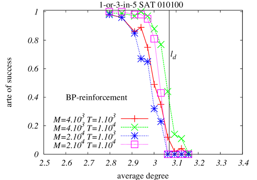
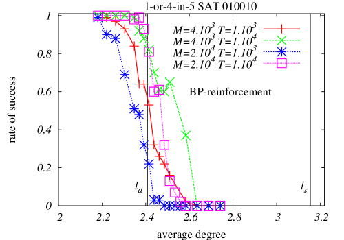
Figure 7: Performance of the BP reinforcement on two of the locked occupation problems. Probability of success versus average connectivity. Left: $A=010100$, the optimal parameters: $\gamma=0.1$, $\pi=0.28$ for $2.79\leq\overline{l}\leq 2.95$, $\pi=0.30$ for $2.97\leq\overline{l}\leq 3.13$, $\pi=0.31$ for $c=3.15$. Right: $A=010010$ with $\gamma=0.1$, $\pi=0.34$. The different curves are for two different system sizes and two different maximal running times. The algorithm performs well only up to a connectivity close to the clustering transition ($l_{d}=3.07$ resp. $l_{d}=2.41$ to be compared with the satisfiability threshold $l_{s}=4.72$ resp. $l_{s}=3.16$). Qualitatively similar result were observed for all the other locked occupation problems we studied.

We tested the BP-Reinforcement algorithm on the locked occupation CSPs, the results are shown in Fig. 7. The fraction of successful runs on different system sizes and for different maximal running times is plotted as a function of the mean variable connectivity. Our data suggest that the algorithm is successful only in the liquid phase, and fails in the clustered (that is also frozen) region. Similar results can be obtained with other algorithms; for instance the performance of stochastic local search was reported in Zdeborová and Mézard (2008).

The clustered phase is thus extremely hard and instances of the locked problems can serve as benchmarks for new solvers. In fact, some of the hardest benchmarks of the K-satisfiability problem are based on a well known LOP, XOR-SAT (with some additional non-linear function nodes which rule out the Gaussian elimination solvers) Haanpää et al. (2006); Barthel et al. (2002).

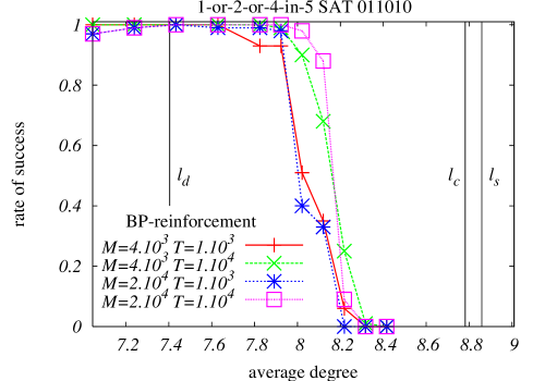
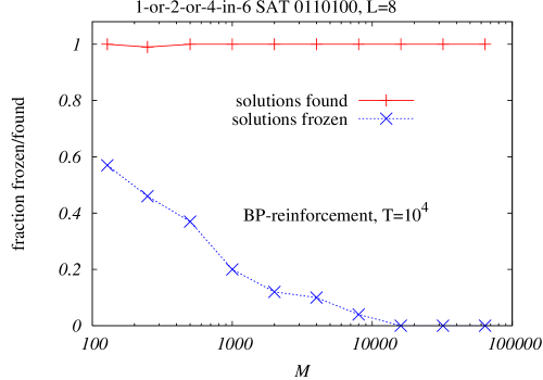
Figure 8: Left: Performance of the BP reinforcement on one of the non-locked problems, $A=010110$. Parameters: $\gamma=0.1$; $\pi=0.40$ for $7.0\leq\overline{l}\leq 7.8$, $\pi=0.42$ for $7.9\leq\overline{l}\leq 8.0$, $\pi=0.44$ for $8.1\leq\overline{l}\leq 8.4$. The implementation of the algorithm is the same as for the locked problems in Fig. 7. Here solutions are found up to about a half of the clustered region, $l_{d}=7.40$. The condensation $l_{c}=8.78$ and the satisfiability $l_{s}=8.86$ transition are also marked. Right: The $A=0110100$ at regular graphs of $L=8$ is in the rigid phase, that is almost all solutions belong to frozen clusters. Yet the BP reinforcement ($\gamma=0.1$, $\pi=0.36$) finds a solution almost surely (after 3 restarts) – the red curve. The blue curve gives a fraction of how many of the solutions found belonged to a frozen cluster. We see that asymptotically we never find the frozen solutions.

In the non-locked problems the very same implementation of the BP reinforcement is able to find solutions inside the clustered region, Fig. 8 left shows the performance for $A=011010$. This is in qualitative agreement with results for the K-SAT Chavas et al. (2005), coloring Krzakala et al. (2007); Zdeborová and Krzakala (2007) or bicoloring problems Dall’Asta et al. (2008).

It is not known how one can characterize from a geometrical point of view the connectivity threshold where BP reinforcement algorithms stop to be efficient in the non-locked problems. It has been found in Dall’Asta et al. (2008) that even the rigid phase where almost all solutions are frozen may be algorithmically easy. Fig. 8 confirms this statement for the problem $A=0110100$ on the regular ensemble with $L=8$. The ratio of success of the BP reinforcement (with 3 restarts) is close to one, and basically independent of system size, while it can be seen from (11) that this problem is in the rigid phase. On the other hand the fraction of found solutions which are frozen (have a nontrivial whitening core Braunstein and Zecchina (2004); Ardelius and Zdeborová (2008)) goes to zero as the system size is growing, in agreement with the results of Dall’Asta et al. (2008). Thus the question of where is the easy/hard threshold in the non-locked problems remains open.

VI Conclusion

We studied the class of occupation CSPs on which we illustrated the difference between locked and non-locked CSPs. The point-like nature of clusters in LOPs is responsible for all of these differences. Our finding may be summarized as: ”Locked problems are extremely simple and extremely hard.” The simplicity comes at the level of the phase diagram, which can be computed by the cavity method much more easily that in the general CSP. In certain cases some non-trivial quantities are probably amenable to a rigorous study along the lines that we sketched – as for example the satisfiability threshold in the balanced locked problems. The hardness is algorithmic, some algorithms – as the BP decimation – fail completely, and even the best known algorithms are not able to find solutions in the clustered phase of the locked problems. Their simple description and algorithmic hardness makes the locked problems challenging for developments of new algorithms as well as for better theoretical understanding on the origin of hardness.

There are several clear directions in which this work should be extended. The planted ensembles of LOPs should be studied in order to provide hard benchmarks where the existence of a solution would be guaranteed. On the mathematical side the rigorous proof of the second moment method giving the satisfiability threshold in the balanced locked problems should be worked out. One may investigate if the location of the clustering threshold can be proven rigorously using the small noise reconstruction in the lines of Sly (2008), or bounding the weight enumerator function in the lines of Mora and Mézard (2006). Also it will be interesting to study (at least numerically) the dynamics at finite temperature, as it might provide further insight into the connection between the dynamics of algorithms and structure of solutions. Finally the distance properties between solutions in locked CSPs makes them interesting candidates for the development of nonlinear error correcting codes or compression schemes.

References

- Cook (1971) S. A. Cook, in Proc. 3rd STOC (ACM, New York, NY, USA, 1971), pp. 151–158.
- Garey and Johnson (1979) M. Garey and D. Johnson, Computers and intractability: A guide to the theory of NP-completeness (Freeman, San Francisco, 1979).
- Cheeseman et al. (1991) P. Cheeseman, B. Kanefsky, and W. M. Taylor, in Proc. 12th IJCAI (Morgan Kaufmann, San Mateo, CA, USA, 1991), pp. 331–337.
- Mitchell et al. (1992) D. G. Mitchell, B. Selman, and H. J. Levesque, in Proc. 10th AAAI (AAAI Press, Menlo Park, California, 1992), pp. 459–465.
- Mézard et al. (1987) M. Mézard, G. Parisi, and M. A. Virasoro, Spin-Glass Theory and Beyond, vol. 9 of Lecture Notes in Physics (World Scientific, Singapore, 1987).
- Mézard et al. (2002) M. Mézard, G. Parisi, and R. Zecchina, Science 297, 812 (2002).
- Biroli et al. (2000) G. Biroli, R. Monasson, and M. Weigt, Eur. Phys. J. B 14, 551 (2000).
- Mézard and Zecchina (2002) M. Mézard and R. Zecchina, Phys. Rev. E 66, 056126 (2002).
- Zdeborová and Krzakala (2007) L. Zdeborová and F. Krzakala, Phys. Rev. E 76, 031131 (2007).
- Zdeborová and Mézard (2008) L. Zdeborová and M. Mézard, Phys. Rev. Lett. 101, 078702 (2008).
- Mulet et al. (2002) R. Mulet, A. Pagnani, M. Weigt, and R. Zecchina, Phys. Rev. Lett. 89, 268701 (2002).
- Krzakala et al. (2007) F. Krzakala, A. Montanari, F. Ricci-Tersenghi, G. Semerjian, and L. Zdeborová, Proc. Natl. Acad. Sci. U.S.A 104, 10318 (2007).
- Montanari et al. (2008) A. Montanari, F. Ricci-Tersenghi, and G. Semerjian, J. Stat. Mech. p. P04004 (2008).
- Mora (2007) T. Mora, Ph.D. thesis, Université Paris-Sud (2007), http://tel.archives-ouvertes.fr/tel-00175221/en/.
- Kschischang et al. (2001) F. R. Kschischang, B. Frey, and H.-A. Loeliger, IEEE Trans. Inform. Theory 47, 498 (2001).
- Mézard and Montanari (2008) M. Mézard and A. Montanari, Information, Physics, Computation: Probabilistic approaches (Cambridge University Press, Cambridge, 2008), in preparation: www.lptms.u-psud.fr/membres/mezard/.
- Raymond et al. (2007) J. Raymond, A. Sportiello, and L. Zdeborová, Phys. Rev. E 76, 011101 (2007).
- Zdeborová and Mézard (2006) L. Zdeborová and M. Mézard, J. Stat. Mech. 5, P05003 (2006).
- Achlioptas and Moore (2006) D. Achlioptas and C. Moore, SIAM Journal on Computing 36, 740 (2006).
- Castellani et al. (2003) T. Castellani, V. Napolano, F. Ricci-Tersenghi, and R. Zecchina, J. Phys. A 36, 11037 (2003).
- Dall’Asta et al. (2008) L. Dall’Asta, A. Ramezanpour, and R. Zecchina, Phys. Rev. E 77, 031118 (2008).
- Marinari and Semerjian (2006) E. Marinari and G. Semerjian, J. Stat. Mech. 6, P06019 (2006).
- Schaefer (1978) T. J. Schaefer, in Proc. 10th STOC (ACM, New York, NY, USA, 1978), pp. 216–226.
- Mézard et al. (2003) M. Mézard, F. Ricci-Tersenghi, and R. Zecchina, J. Stat. Phys. 111, 505 (2003).
- Connamacher and Molloy (2004) H. Connamacher and M. Molloy, in 45th Symposium on Foundations of Computer Science (FOCS 2004), 17-19 October 2004, Rome, Italy, Proceedings (IEEE Computer Society, 2004), ISBN 0-7695-2228-9.
- Mézard and Parisi (2001) M. Mézard and G. Parisi, Eur. Phys. J. B 20, 217 (2001).
- Pearl (1982) J. Pearl, in Proceedings American Association of Artificial Intelligence National Conference on AI (Pittsburgh, PA, USA, 1982), pp. 133–136.
- Mézard and Montanari (2006) M. Mézard and A. Montanari, J. Stat. Phys. 124, 1317 (2006).
- Mossel (2001) E. Mossel, Ann. Appl. Probab. 11, 285 (2001).
- Zdeborová (2007) L. Zdeborová, Ph.D. thesis, Université Paris-Sud (2007), arXiv:0806.4112v1 [cond-mat.stat-mech].
- Semerjian (2008) G. Semerjian, J. Stat. Phys. 130, 251 (2008).
- Achlioptas et al. (2005) D. Achlioptas, A. Naor, and Y. Peres, Nature 435, 759 (2005).
- Achlioptas and Ricci-Tersenghi (2006) D. Achlioptas and F. Ricci-Tersenghi, in Proc. of 38th STOC (ACM, New York, NY, USA, 2006), pp. 130–139.
- Ardelius and Zdeborová (2008) J. Ardelius and L. Zdeborová, Phys. Rev. E (Rapid Com.) p. 040101(R) (2008).
- Krauth and Mézard (1989) W. Krauth and M. Mézard, J. Phys. France 50, 3057 (1989).
- Martin et al. (2004) O. C. Martin, M. Mézard, and O. Rivoire, Phys. Rev. Lett. 93, 217205 (2004).
- Martin et al. (2005) O. C. Martin, M. Mézard, and O. Rivoire, J. Stat. Mech. p. P09006 (2005).
- Zhou and Ou-Yang (2003) H. Zhou and Z. Ou-Yang (2003), preprint arXiv:cond-mat/0309348v1 [cond-mat.dis-nn].
- Mora and Mézard (2006) T. Mora and M. Mézard, J. Stat. Mech. 10, P10007 (2006).
- Di et al. (2006) C. Di, T. J. Richardson, and R. Urbanke, IEEE Trans. Inform. Theory 52, 4839 (2006).
- Montanari and Ricci-Tersenghi (2003) A. Montanari and F. Ricci-Tersenghi, Eur. Phys. J. B 33, 339 (2003).
- Rivoire et al. (2004) O. Rivoire, G. Biroli, O. C. Martin, and M. Mézard, Eur. Phys. J. B 37, 55 (2004).
- Krzakala and Zdeborová (2008) F. Krzakala and L. Zdeborová, Eur. Phys. Lett. 81, 57005 (2008).
- Achlioptas et al. (2001a) D. Achlioptas, A. Chtcherba, G. Istrate, and C. Moore, in SODA ’01: Proceedings of the twelfth annual ACM-SIAM symposium on Discrete algorithms (SIAM, Philadelphia, PA, USA, 2001a), pp. 721–722.
- Cocco et al. (2003) S. Cocco, O. Dubois, J. Mandler, and R. Monasson, Phys. Rev. Lett. 90, 047205 (2003).
- Achlioptas et al. (2001b) D. Achlioptas, L. M. Kirousis, E. Kranakis, and D. Krizanc, Theoretical Computer Science 256, 109 (2001b).
- Parisi (2003) G. Parisi (2003), arXiv:cs/0301015.
- Chavas et al. (2005) J. Chavas, C. Furtlehner, M. Mézard, and R. Zecchina, J. Stat. Mech. p. P11016 (2005).
- Eén and Sorensson (2004) N. Eén and N. Sorensson, in Theory and Applications of Satisfiability Testing (Springer Berlin, Heidelberg, 2004), pp. 502–518.
- Montanari et al. (2007) A. Montanari, F. Ricci-Tersenghi, and G. Semerjian (2007), to appear in Proceedings of Allerton 2007. Preprint: arXiv:0709.1667v1 [cs.AI].
- Braunstein and Zecchina (2006) A. Braunstein and R. Zecchina, Physical Review Letters 96, 030201 (2006).
- Haanpää et al. (2006) H. Haanpää, M. Järvisalo, P. Kaski, and I. Niemelä, Journal on Satisfiability, Boolean Modeling and Computations 2, 27 (2006).
- Barthel et al. (2002) W. Barthel, A. K. Hartmann, M. Leone, F. Ricci-Tersenghi, M. Weigt, and R. Zecchina, Phys. Rev. Lett. 88, 188701 (2002).
- Braunstein and Zecchina (2004) A. Braunstein and R. Zecchina, Journal of Statistical Mechanics: Theory and Experiment p. P06007 (2004).
- Sly (2008) A. Sly (2008), arXiv:0802.3487v1 [math.PR].
- Janson and Mossel (2004) S. Janson and E. Mossel, Ann. Probab. 32, 2630 (2004).