On the accuracy of the high redshift cluster luminosity function

Abstract

We study the reliability of the statistical background subtraction method for computing the Ks-band luminosity function of cluster galaxies at $z\sim 1$ using mock Red-sequence Cluster Survey cluster catalogues constructed from GALFORM semi-analytic galaxies. The underlying cluster luminosity function in the mocks are compatible with recent estimates at $z\sim 1$ by several authors. We simulate different samples where the number of clusters with Ks-band photometry goes from $5$ to a maximum of $50$, in order to find the most suitable observational sample to carry out this study; the current observational status in the nIR wavelength range has been reached using $5$ real clusters at $z\sim 1$. We compute the composite luminosity function for several samples of galaxy clusters with masses $\simeq 1.5\times 10^{14}M_{\odot}$ assuming a flux limited, complete sample of galaxies down to ${\rm Ks}=21.0$ magnitudes. We find that the Schechter fit parameters $\mathrm{Ks}^{*}$ and $\alpha$ for a sample of galaxies with no redshift information are rather poorly constrained if both parameters are allowed to vary freely; if $\alpha$ is fixed at a fiducial value, then $\mathrm{Ks}^{*}$ shows significantly improved stochastic uncertainties but can be influenced by systematic deviations. We find a significantly improved accuracy in the luminosity function parameters when adding photometric redshift information for bright cluster galaxies. The impact of a ten-fold increase in the number of clusters with available Ks-band photometry is that of decreasing stochastic errors in $\mathrm{Ks}^{*}$ and $\alpha$ by factors of $\simeq 2$ and $\simeq 4$, respectively, for accuracies of up to $\left(\Delta\mathrm{Ks}^{*}/\mathrm{Ks}^{*}\right)_{\rm stochastic}=0.02$ and $\left(\Delta\alpha/\alpha\right)_{\rm stochastic}=0.09$. The dwarf-to-giant ratios inferred from the luminosity functions of red-sequence galaxies in the mock catalogue agree very well with the underlying values; however, there is an indication that the semi-analytic model over-predicts the abundance of dwarf galaxies by up to a factor of $3$ with respect to recent measurements. Finally, we find that in order to use estimates of ${\rm Ks}^{*}$ to study the formation redshift of cluster galaxies at $z=1$, the sample would need to contain 520 $z\sim 1$ clusters, for an accuracy of $\sim 2\;\mathrm{Gyr}$ at the 68 per cent confidence level. However, combining this method with other estimates may reduce significantly the sample size, and allow important new constraints on galaxy formation models.

1 Introduction

The galaxy luminosity function (LF) is one of the fundamental quantities of observational cosmology. Its evolution with redshift and dependence on galaxy morphology and environment has been extensively used to provide strong constraints on galaxy evolution models.

Clusters of galaxies are the largest virialised structures at any given epoch, which grow from high-density regions in the primordial matter distribution of the Universe, and may have formed between $9\;\mathrm{Gyrs}$ ago and the present (Stanford et al., 2006). Most of them have been detected in surveys carried out in the X-ray (Romer et al. 2001, Barkhouse et al. 2006) and optical bands (Postman et al. 1996, Gonzalez et al. 2001, Gladders & Yee 2005), and it is expected that upcoming Sunyaev-Zel’dovich surveys will yield thousands of galaxy clusters (Carlstrom et al., 2002). The fact that clusters contain large numbers of galaxies practically at the same distance from the observer within a small area on the sky, makes them ideal systems to study the LF down to very faint magnitudes.

In the local Universe, the LF of cluster galaxies has been studied extensively by Goto et al. (2002) and De Propris et al. (2003), who found that there is no significant evidence for variations in the LF across a broad range of cluster properties, and also, that the cluster LF differs significantly from the field LF. Although many efforts have been done to perform such a study at $z\sim 1$, a significant look-back time of $7\;\mathrm{Gyrs}$ in the currently favoured cosmology, only a handful of high redshift clusters have been detected to date in optical and X-ray surveys (Stanford et al. 1997, Toft et al. 2004, De Propris et al. 2007). Recently, Eisenhardt et al. (2008) found 106 galaxy clusters and groups candidates at $z>1$ in the Spitzer Infrared Camera (IRAC) Shallow Survey (Eisenhardt et al., 2004).

Obtaining spectroscopic measurements for a large number of faint cluster galaxies at $z\sim 1$ is a very difficult and time-expensive task. As a consequence, to date there are no reliable LFs measured at $z\sim 1$ using only spectroscopically confirmed members. Several authors have attempted to solve this issue by using photometric redshifts to define cluster membership and to compute the LF (Toft et al. 2004, Tanaka et al. 2007), but their results have been criticised due to the unknown spectral energy distribution (SED) of galaxies at high redshifts (Andreon et al. 2005, Sheth 2007).

Traditionally, the cluster LF is computed applying a background subtraction method, which consists of computing the difference between galaxy counts in the cluster and control field directions. Several authors have developed and applied their own subtraction methods (Oemler 1974, Pimbblet et al. 2002, Andreon et al. 2005). However, it is difficult to assess whether this method is free of important systematic effects due to possible problems in the background subtraction method, which needs to select an appropriate area, either around the clusters under study or from an independent large area photometric sample.

It has been claimed that infrared luminosities are better suited to measure the LF than their optical counterparts, since the former are comparatively insensitive to the star formation history while reflecting the total stellar mass (Charlot 1996, Madau, Pozzetti, & Dickinson 2004). Furthermore, infrared luminosities have a negligible extinction correction and their K-correction depends only weakly on Hubble type (see for instance Mannucci et al. 2001).

The main goal of this work is to study the reliability of the statistical background subtraction method to recover the underlying observer-frame Ks-band LF. Section 2 explains the mock catalogues in which we base our analysis. Section 3 discusses the background subtraction method and shows the resulting LF estimates, and Section 4 shows a comparison between the underlying and recovered LF, and several physical quantities inferred from the LF. Our conclusions are summarized in Section 5.

Throughout this paper we assume $\Omega_{M}=0.3$, $\Omega_{\Lambda}=0.7$ and $H_{0}=70~{}km\,s^{-1}\,Mpc^{-1}$. All magnitudes are in the Vega system.

2 Data

This work concentrates in particular, on the possibility to study the LF of $z\simeq 1$ clusters, in such a way so as to obtain the accuracy needed to study different properties of the galaxy population including the relative importance of dwarf vs. giant galaxies (De Lucia et al. 2007, Gilbank & Balogh 2008a), or the expected formation redshift of $z\sim 1$ cluster galaxies. To date, the most suited cluster survey for such a study is the Red sequence Cluster Survey (RCS-1, Gladders et al. 2005) However, there is only optical information for these clusters, so a study of the LF over the infrared wavelength range would require an observing campaign to obtain these data. The authors of this work are at the moment in the process of obtaining such information, so that this study will be possible in the near future.

2.1 Mock catalogues

In order to test for possible systematic errors affecting a statistical measurement of the cluster LF, we apply this analysis to mock RCS catalogues. We construct mock RCS catalogues using the Millennium simulation (Springel, Frenk & White, 2006) populated with semi-analytic galaxies from the GALFORM model by Baugh et al. (2005) (see also Cole et al. 2000, Bower et al. 2006; for an alternative approach see Lagos, Cora & Padilla 2008). The numerical simulation follows the gravitational interaction of $10^{9}$ dark-matter particles in a $\Lambda$CDM Universe characterized by the cosmological parameters $\Omega_{m}=0.30$, $\Omega_{\Lambda}=0.70$, a power law spectral index $n=0.94$, an amplitude of matter density fluctuations in spheres of $8\;\mathrm{h}^{-1}\,\mathrm{Mpc}$, $\sigma_{8}=0.8$, and a Hubble constant $H_{0}=100\;h\,\mathrm{km}\,\mathrm{s}^{-1}\,\mathrm{Mpc}^{-1}$ with $h=0.70$. The GALFORM semianalytic model was applied to the merger trees of halos in the simulation, which have a minimum mass of $1.2\times 10^{10}\;\mathrm{h}^{-1}\,\mathrm{M}_{\odot}$ for a minimum of 20 dark-matter particles (courtesy of the Durham group). The galaxies in the simulation are characterized by their luminosity in several photometric bands, including the near infrared Ks-band and those available in the RCS dataset. In order to construct each mock catalogue, we place an observer in the simulation, and record all angular positions of galaxies down to the RCS magnitude limit within an area of $100$ square degrees. The intrinsic completeness limit in our mock catalogues is $\mathrm{Ks}=22.0$, observer-frame, following the resolution constraints of the semi-analytic galaxy population. Notice that this limit can be lowered to meet the restrictions of a given observational sample.

In order to include the evolution of the galaxy population with redshift, we use simulation outputs corresponding to four different redshifts from $z=0.3$ to $z=3$ for consecutive redshift ranges. This ensures that the population of background galaxies behind our mock RCS clusters are characterized by an evolving luminosity function to distances beyond the maximum expected galaxy redshifts allowed by the magnitude limit cut. The fact that we are not interested in the differential evolution of the luminosity function with redshift justifies our choice of mock light-cones with discretised evolution.

The advantage of using mock catalogues relies in that the underlying population of clusters is known, along with the LF parameters for the field and cluster environments for each individual mock. Furthermore, as we are using multiple mocks extracted from practically independent volumes in the simulation, we can estimate the expected effects of sample variance in our statistics. Besides these advantages, we are also able to make a comparison between the properties of galaxies populating the mocks and those in real datasets published in previous works, providing a new test for the GALFORM semi-analytic model.

Since we are interested in employing these mock catalogues to study the accuracy of the background subtraction method for computing the galaxy LF for RCS-1 clusters, we compare the mass function between simulated and observed clusters. Figure 1 shows the mass function of simulated clusters selected from the mock catalogues and RCS-1 observed clusters taken from Gladders et al. (2007), where it can be seen that both mass functions are roughly compatible for $M_{200}>1.5\times 10^{14}\,M_{\odot}\,h^{-1}$ to a $1\,\sigma$ level. The offset in the observational data can be due in part to errors in the mass measurements which usually broaden statistical distributions (see for instance Padilla & Lambas (1999))

Figure 1: Mass function of simulated and observed clusters. The filled circles show the mass function of simulated clusters selected from the mock catalog. The open triangles show the mass function of observed clusters selected from the RCS-1 cluster catalog (Gladders et al., 2007).

3 Luminosity function estimates

The optimal method to build a reliable cluster LF consists in using spectroscopic information to determine cluster membership. However, obtaining spectroscopic redshifts for a large number of faint galaxies at high redshifts is prohibitively expensive in telescope time.

The cluster samples in our mock catalogues are characterized by a $z=1$ LF in the Ks-band which we fit with a Schechter function of characteristic luminosity $\mathrm{Ks}^{*}=18.27$ and faint-end slope $\alpha=-1.36$. Our approach to determine the reliability of different LF estimators takes advantage of our knowledge of the underlying LF parameters. We notice that the characteristic luminosity in the model is in good agreement with the observational result $\mathrm{Ks}^{*}=18.5\pm 1.2$ found by Strazzullo et al. (2006), who applied a background subtraction method and fitted for both, the characteristic luminosity ${\rm Ks^{*}}$ and $\alpha$, the faint-end slope. Other measurements show different levels of agreement; for instance, Kodama et al. (2003) found a fainter value $\mathrm{Ks}^{*}=17.57\pm 0.24$, using a fixed value of $\alpha=-0.9$ and relatively shallow nIR data. With respect to the faint-end slope, this parameter is poorly constrained by observational data, and consistent with $\alpha=-1$. Therefore, down to the accuracy of the observational results, the semi-analytic model used to construct the mock catalogues is able to reproduce the observed cluster galaxy population at $z\simeq 1$.

In the following subsection we discuss two possible LF estimators that we will apply to the mock cluster catalogues.

3.1 Background subtraction and photometric redshift LF estimators

Two widely used methods to calculate the LF are the statistical background subtraction and the photometric redshift method. The former consists on using one or several control fields to determine the number of contaminating galaxies (background and foreground galaxies) per unit area as a function of magnitude, to then compute the galaxy LF as the difference between the galaxy number count in the cluster direction and the control field. This is the method of choice when there is photometry in only one or two bands for galaxies in the cluster direction, and very few cluster members have been spectroscopically confirmed. Employing numerical simulations, it has been shown that the background subtraction method can recover accurately the underlying LF of clusters selected in three dimensions (Valotto et al., 2001).

The background subtraction method requires to define a magnitude bin width, a cluster-centered aperture, and a control field region. When computing the number counts in the cluster direction for the RCS mock catalogue, we mimic the observational method of employing galaxies enclosed by a circular aperture of radius $0.27\;\mathrm{h}^{-1}\;\mathrm{Mpc}$ centered on the brightest cluster galaxy and a magnitude bin of width $0.5\;\mathrm{mag}$. This aperture size is justified because the nIR imaging of RCS clusters covers only $0.8\;\mathrm{h}^{-1}\;\mathrm{Mpc}$ of the cluster central region. We defined the control field region based in the observational nIR surveys to date, which should have a minimum $5\sigma$ limiting magnitude of $\mathrm{Ks}=22.0$ and cover a big area in the sky. The candidates were the Faint Infrared Extragalactic Survey (FIRES; Labbé et al. 2003), which covers $8.3\;\mathrm{arcmin}^{2}$ and reaches a $5\sigma$ depth for point sources of $\mathrm{Ks_{5\sigma}}=24.5$; the Great Observatories Origins Deep Survey of CDF-S region (GOODS/ISAAC; Retzlaff et al. 2008), which covers $170\;\mathrm{arcmin}^{2}$ and reaches $\mathrm{Ks_{5\sigma}}=22.8$; and the nIR VIMOS-VLT Deep Survey (VVDS-NIR; Iovino et al. 2005), which covers $430\;\mathrm{arcmin}^{2}$ and reaches $\mathrm{Ks_{5\sigma}}=22.1$. Figure 2 shows the ratio between the rms variation of number count along the control field regions previously mentioned and the rms variation of actual cluster members in the mock. We can see that a control field of size the FIRES survey contributes about $30\%$ to the rms variation along the cluster direction, so the accuracy of the LF built from a background subtraction method would be highly limited by the small control field region. Also, in order to reach a $0.4\%$ contribution of background rms variation to the Ks-band LF error bars we would need a nIR survey covering $1\;\mathrm{deg}^{2}$, which does not even exist at this magnitude depth to date. This way, GOODS/ISAAC and VVDS-NIR are the most suitable surveys to build the Ks-band LF with about $100\%$ completeness to magnitude 21.0 using the background subtraction method.

We discard the VVDS-NIR survey, since the calibrated images of GOODS are publicly available and are taken with the same instrument as the nIR imaging of the RCS clusters (Muñoz et al., 2008)

Using the mock catalogues, we compute the rms variation of number counts from several $170\;\mathrm{arcmin}^{2}$ regions in the mock catalogues, and compare this to Poisson errors and jacknife algorithm estimates (see Figure 3, top panel). It can be seen that a Poisson distribution underestimates the actual rms variation about $30\%$ and $60\%$ for bright and faint galaxies, respectively. This high discrepancy can be explained by the galaxy-galaxy correlation and the presence of large scale structure along the control field region (see for instance, Padilla et al. 2004, Paz, Stasyszyn & Padilla 2008). We also see that the jacknife algorithm reproduces the underlying spread in number counts seen in the simulation to a higher degree. This way, the error in the galaxy count along the control field region, $\sigma_{N_{f}}$, will be computed from the jacknife algorithm.

Figure 2: Ratio between the rms variation of number counts along the control field regions of several sizes and the rms variation of actual cluster members. Open circles correspond to the deepest nIR survey FIRES, stars correspond to the public ESO survey of the CDF-S region GOODS/ISAAC, and triangles to the deep and wide VVDS. The squares correspond to an hypothetical nIR survey covering $1\;\mathrm{deg}^{2}$, reaching a $5\sigma$ limiting magnitude deeper than $\mathrm{Ks}=22.0$

The observational program being carried out to obtain near-infrared imaging of RCS clusters (Muñoz et al. 2008) will only cover fields centered in clusters, therefore, it is important to test whether the use of number counts from a different source catalogue will still allow measuring the LF with minimum systematic deviations from the underlying values.

The number of clusters members along the cluster direction in the $j^{th}$ magnitude bin $N_{j}$, and its error, $\sigma_{N_{j}}$, are given by

$$N_{j} = N_{dj}-N_{fj}\frac{\Omega_{d}}{\Omega_{f}}$$ (1)

$$\sigma_{N_{j}} = \sqrt{\sigma_{N_{dj}}^{2}+\left(\sigma_{N_{fj}}\frac{\Omega_{d}}{\Omega_{f}}\right)^{2}},$$ (2)

where $N_{dj}$ is the number of galaxies (cluster+field) in the cluster direction in the $j^{th}$ bin, $N_{fj}$ is the number of galaxies in the control field region in the $j^{th}$ bin, $\Omega_{d}$ is the area of the cluster-centered circular aperture, and $\Omega_{f}$ is the area of the control field region. The error in the number counts in the cluster direction, $\sigma_{N_{dj}}$, is estimated by the Poissonian error, a choice we justify next.

Figure 3: rms variation in the galaxy counts along the control field region of size the GOODS/ISAAC survey (top panel) and along the cluster direction (bottom panel) as function of magnitude. The solid line shows the actual dispersions built from $100$ independent mock samples. The dashed and dotted lines in the top panel show the errors in the background number count estimated from the classical Poissonian error $\sqrt{N}$ and from applying a jacknife technique, respectively. The dashed and dotted lines in the bottom panel show the errors in cluster direction number count estimated from the classical and a modified Poissonian error $1+\sqrt{N+0.75}$

We calculate the counts in the cluster direction for $100$ independent samples containing $10$ RCS clusters each, and calculate the dispersion in these counts as a function of apparent magnitude. We then select one of these samples at random, which we use to compute the classical Poisson error $\sqrt{N}$ for the number counts in the cluster direction, and the modified Poisson error $1+\sqrt{(N_{dj}+0.75)}$ proposed by Gehrels (1981) and employed by several authors (Andreon et al. 2005, Strazzullo et al. 2006). The bottom panel of Figure 3 shows the comparison between the dispersion in the counts in the cluster direction and its estimated error as a function of the observed magnitude. From this figure we conclude that the classical Poisson error resembles best the dispersion in the mocks, while the modified Poisson errors overestimates errors by a significant amount. Therefore, this justifies our choice of Poisson errors when studying the cluster counts in the mock CLFs. Zheng et al. (2005) find that the number of galaxies in dark matter haloes in semi-analytic and SPH simulations follows a Poisson distribution, which would indicate that galaxies outside the cluster (either in front or behind due to projection effects) only contribute a relatively low fraction of the uncertainty in the cluster counts.

Figure 4: Completeness (solid line) and failure ratio (dashed line) of photometric redshift method as function of Ks-band magnitude. The open circles correspond to cluster members candidates lying 1 $\sigma_{z/(1+z)}$ from the cluster redshift, while the triangles and squares correspond to galaxies lying 2 and 3 $\sigma_{z/(1+z)}$, respectively.

The photometric redshift method consists of using broad-band photometry in several band-passes as a very low resolution spectrum, and then fitting a spectral energy distribution (SED) template to estimate the redshift of the galaxies in the cluster field. The final step consists on defining as cluster members those galaxies lying within a redshift shell centered on the cluster redshift. For simplicity , we do not compute the photometric redshifts of galaxies from fitting a SED to the observed magnitudes but rather from perturbing their actual redshifts by a gaussian distribution with $\sigma_{z/(1+z)}=0.05\,$. It is important to note that the true probability distributions of photometric redshifts are often highly non-Gaussian, and that secondary maxima or extended wings might change the accuracy of photometric redshift method used in this paper. Figure 4 shows the completeness and failure ratio of the photometric redshift method computed from 500 independent Monte-Carlo realizations of photometric redshift of randomly selected clusters. Each realization consists in choosing a random cluster located at $z\sim 1$, then selecting those galaxies within a circular aperture of radius $0.27\;\mathrm{h}^{-1}\;\mathrm{Mpc}$, and finally, simulate their photometric redshifts using the actual redshifts from the mock catalogues via a Monte-Carlo procedure. We can see that the photometric redshift cut $\textrm{1-}\sigma_{z/(1+z)}$ recovers a low percentage of actual cluster galaxies and has a failure ratio of about 10 percent, while the redshift cut of $\textrm{2-}\sigma_{z/(1+z)}$ recovers almost all the actual cluster galaxies and has a failure ratio of about 15 percent. The cut of $\textrm{3-}\sigma_{z/(1+z)}$ has the highest completeness, but the failure ratio of bright galaxies increases rapidly. According to the previous considerations, we define as cluster members those galaxies lying within $\textrm{2-}\sigma_{z/(1+z)}$ from the cluster redshift. Large scale structure plays a role in this calculations and therefore a simple analytic gaussian is only approximate.

The RCS clusters under study by Muñoz et al. (2008) have deep J and Ks-band imaging, and shallow $\rm R_{C}$ and z imaging, so it is not possible to build the LF up to magnitude $Ks=21.0$ from applying the photometric redshift method. In order to take advantage of the available data, we propose a new method that consists in using photometric redshift of galaxies to compute the bright part of the LF and using the background subtraction method to compute the faint part. The cluster members with $\rm{Ks}\leq 18.5$ are identified by their photometric redshift, while the number of members with $\rm{Ks}>18.5$, by using the background subtraction method. The combination of both methods will be called B+Z method hereafter.

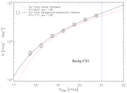
Figure 5: Ks-band composite luminosity function (CLF) built from the background subtraction and B+Z methods. Shown are the CLF built from the background subtraction method for 5 clusters (top-left), for 10 clusters (top-right), and for 50 clusters (bottom-left). Also, the CLF built from the B+Z method for 50 clusters (bottom-right). Dashed line shows the underlying CLF, while open squares show the recovered CLF from applying the respective method.

3.2 The composite luminosity function

In most galaxy clusters there are too few galaxies to determine accurately the shape of the LF. A solution to this problem is to measure the LF using a combined sample of clusters, allowing a higher precision measurement. This method is commonly known as the Composite Luminosity Function (CLF) method.

The CLF is built according to the following formulation,

$$N_{cj}=\frac{1}{n_{j}}\sum_{i=1}^{N_{clusters}}N_{ij},$$ (3)

where $N_{cj}$ is the number of galaxies in the j-th bin of the CLF, $N_{ij}$ is the number of galaxies in the j-th bin of the i-th cluster, and $n_{j}$ is the number of clusters with limiting magnitude deeper than the j-th bin. The formal errors of the CLF were computed according to,

$$\sigma_{N_{cj}}=\frac{1}{n_{j}}\sqrt{\sum_{i=1}^{N_{clusters}}\sigma_{N_{ij}}^{2}}$$ (4)

where $\sigma_{N_{ij}}$ is the formal error of the number of galaxies in the j-th bin of the i-th cluster.

For computing the CLF, we selected several galaxy clusters with masses about $1.5\times 10^{14}\;\mathrm{M}_{\odot}$, located between redshifts $0.90<z<1.10$. The observed CLF was built for 3 cluster samples taken from the mocks: the first sample contains 5 clusters (CS1), the second, 10 clusters (CS2), and the third, 50 clusters (CS3). We reset the completeness limit in our mock catalogues to $\mathrm{Ks}=21.0$ in order to match the RCS nIR imaging (Muñoz et al. 2008), and we apply both, the background subtraction and B+Z methods for computing the CLF.

Figure 5 shows the resulting CLF computed for a CS3 dataset, using both the background subtraction and B+Z methods (upper and lower panels, respectively). The open symbols correspond to the underlying CLF calculated using all the cluster members, and the filled circles correspond to the CLF obtained using only data available in observational samples. This figure will be discussed into more detail in the following section.

4 Analysis

4.1 Schechter parameters

In order to study the reliability of the background subtraction and B+Z methods to recover the underlying LF, we fit a Schechter function to the observed CLF and then compare the best fitting observed parameters to those of the underlying CLF.

The best fitting parameters are found using a minimum $\chi^{2}$ method given by,

$$\chi^{2} = \sum_{j=1}^{N_{bins}}\left(\frac{N_{cj}-N(m_{j};m^{*};\alpha)}{\sigma_{N_{cj}}}\right)^{2},$$ (5)

$$N(m_{j};m^{*};\alpha) = \int_{m_{j}-\frac{m_{bin}}{2}}^{m_{j}+\frac{m_{bin}}{2}}\phi(m)dm,$$ (6)

where $N(m_{j};m^{*};\alpha)$ is the predicted value of the CLF at the magnitude bin $m_{j}$, $m_{bin}$ is the magnitude bin size, and $\phi(m)$ is the Schechter function.

We search the global minimum in the full $\phi^{*}-m^{*}-\alpha$ space sampled by a parameter grid. The best-fitting parameters after marginalizing over $\phi^{*}$, for $\mathrm{Ks}^{*}$ and $\alpha$ taken as free parameters, are summarized in the Table 1 for the three samples of mock galaxy clusters defined in the previous Section. The systematic errors are defined as the difference between the actual and estimated value, while the stochastic errors are defined by the 68 percent confidence levels.

Table 1: Best-fitting parameters for $\mathrm{Ks}^{*}$ and $\alpha$ as free parameters.

Dataset	Param	Actual	Background	B+Z
			method	method
CS1	$K^{*}$	18.27	$18.95^{+0.90}_{-1.23}$	$18.94^{+0.76}_{-0.86}$
	$\alpha$	-1.36	$-1.11^{+0.61}_{-0.46}$	$-1.10^{+0.55}_{-0.41}$
CS2	$K^{*}$	18.27	$17.98^{+0.80}_{-2.27}$	$18.56^{+0.46}_{-0.67}$
	$\alpha$	-1.36	$-1.45^{+0.30}_{-0.28}$	$-1.29^{+0.28}_{-0.27}$
CS3	$K^{*}$	18.27	$17.71^{+0.46}_{-0.71}$	$18.18^{+0.31}_{-0.39}$
	$\alpha$	-1.36	$-1.50^{+0.13}_{-0.12}$	$-1.41^{+0.12}_{-0.12}$

Table 2: Best-fitting parameters derived with a fixed value of $\alpha=-1.36$

Dataset	Param	Actual	Background	B+Z
			method	method
CS1	$K^{*}$	18.27	$18.40^{+0.33}_{-0.39}$	$18.50^{+0.24}_{-0.28}$
CS2	$K^{*}$	18.27	$18.30^{+0.17}_{-0.19}$	$18.42^{+0.15}_{-0.13}$
CS3	$K^{*}$	18.27	$18.20^{+0.09}_{-0.09}$	$18.30^{+0.08}_{-0.06}$

Figure 6 shows the 1- and 2-$\sigma$ likelihood contours of the Schechter function parameters for our sample CS3 using both, the background subtraction and B+Z methods. The plus symbols mark the actual CLF parameters and the crosses mark the best fitting observed CLF parameters. From this figure, we can conclude that the B+Z method gives more accurate and better constrained results than the background subtraction method, since the stochastic error of $\mathrm{Ks}^{*}$ is reduced by almost a factor or $2$.

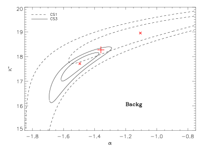
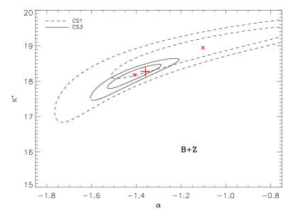
Figure 6: Contour plots showing the constraints on the Schechter function parameters derived from the $\chi^{2}$ minimization analysis applied to the CLF obtained using 5 clusters (dashed line) and 50 clusters (solid line). The upper panel shows the results from applying the statistical background subtraction method; the lower panel shows the results from applying the B+Z method. The plus sign marks the parameters of the true underlying CLF, and the cross marks the best fitting parameters of the measured CLF. The labeled contours represent the 1- and 2-$\sigma$ confidence levels.

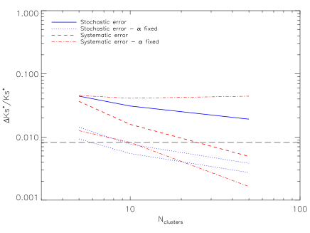
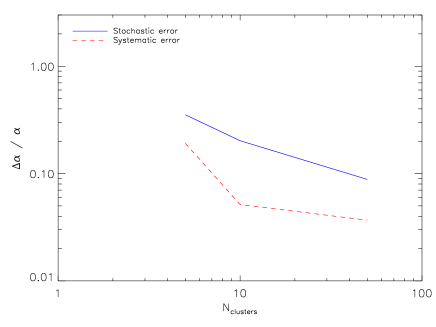
Figure 7: Upper panel: Stochastic and systematic errors in $\mathrm{Ks}^{*}$ obtained through the B+Z LF measurement method, for samples composed by different number of galaxy clusters, for a fixed or free value of the $\alpha$ parameter (line types are shown in the figure key). Upper and lower dotted lines show the stochastic errors in $\mathrm{Ks}^{*}$ for fixed values of $\alpha=-1.36$ and $\alpha=-1.00$ respectively. Upper and lower dot-dashed lines are the systematic error in $\mathrm{Ks}^{*}$ for $\alpha=-1.00$ and $-1.36$, respectively. The horizontal long-dashed line is the maximum error that still allows to distinguish between passive evolution scenarios with formation redshifts of $z_{f}=2$ and $z_{f}=5$. Lower panel: Stochastic and systematic errors in $\alpha$.

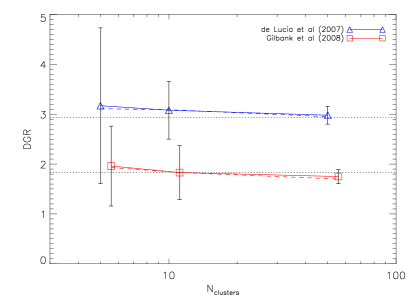
Figure 8: Dwarf-to-giant ratio (DGR) for red-sequence cluster galaxies computed from background subtraction (solid line) and photometric redshift (dashed line) methods. The triangles and squares correspond to the DGR estimated from applying the magnitude limits by De Lucia et al. (2007) and Gilbank et al. (2008b), respectively. The underlying value is shown by the dotted line. The error-bars show the stochastic errors. A small horizontal offset was applied to the Gilbank et al. (2008b) results to improve clarity.

It is useful to study the reliability of the best LF measurement method (B+Z estimator) as a function of the number of galaxy clusters used for computing the CLF, since this can have a direct impact on current and future observational campaigns. In principle, a larger sample of clusters should put better constraints on the values of $\mathrm{Ks}^{*}$ and $\alpha$ as well as lower systematic errors. Figure 7 shows the stochastic and systematic errors for both $\mathrm{Ks}^{*}$ and $\alpha$. From this figure we can conclude that the method reliability and accuracy depend strongly on the number of galaxy clusters, as increasing the sample size by a factor of $10$ reduces the stochastic and systematic errors in $\mathrm{Ks}^{*}$ by factors of $3$ and $30$, respectively.

When the parameter $\alpha$ is fixed to the true underlying value, errors also improve, for instance, by a factor of $3$ in the characteristic luminosity. The results for the three samples of mock galaxy clusters are summarized in Table 2. In the case where the value of $\alpha$ is unknown and a fiducial value $\alpha=-1$ is assumed (as may be the case in an observational estimate of the CLF), the systematic errors increase significantly due to the likelihood degeneracy in the $\mathrm{Ks}^{*}$-$\alpha$ plane, which in our mocks forces the resulting characteristic luminosity to a fainter value. It is also noticeable that in this case, the stochastic error is lower than when fixing $\alpha$ to the true underlying values; this indicates that even though the uncertainties in $\mathrm{Ks}^{*}$ diminish when fixing $\alpha$, if this parameter is offset by only a $23\%$ of its value, there could be significant systematic errors in $\mathrm{Ks}^{*}$ producing biased analyses.

Regarding the faint-end slope, $\alpha$, the stochastic and systematic errors also diminish by about a factor of $4$ when increasing the sample from $5$ to $50$ clusters. It is important to notice that regardless of the number of clusters in the sample, the stochastic error is always found to be larger than systematic deviations.

4.2 Mean formation epoch

The study of the evolution of the CLF is a powerful tool to improve our knowledge on the processes of galaxy formation and evolution, in particular in high density regions of the Universe where the probability of galaxy interactions with their environment is at its highest. In addition, these studies are easier to interpret when using infrared luminosities, since these are better suited than optical photometry to measure the LF, since the former reflect the total stellar mass of galaxies and do not depend strongly on the details of their stellar populations (Gavazzi, Pierini & Boselli, 1996).

One of the most interesting quantities that can be inferred from the evolution of the LF is the mean redshift of the bulk of star formation in cluster galaxies, $z_{f}$; this redshift is defined as a measurement of the time when these galaxies have already acquired most of their stellar mass. This is most easily obtained from observational estimates of the evolution of $\mathrm{Ks}^{*}$ by direct comparison to predictions using passive evolution models with different $z_{f}$.

We employ the passive evolution models of Kodama & Arimoto (1997) to compute the minimum number of galaxy clusters needed to distinguish between a scenario with $z_{f}=2$ and $z_{f}=5$ for the galaxies in our mock catalogues. According to these models, for a $\mathrm{L}^{*}$ galaxy observed at $z=1$, the difference in $\mathrm{Ks}^{*}$ between both scenarios is about 0.3 mag. Therefore, in order to compute $z_{f}$ with an accuracy of $2\;\mathrm{Gyr}$ at the 68 percent confidence level, the maximum systematic and stochastic errors allowed on $\mathrm{Ks}^{*}$ would be $\Delta\mathrm{Ks}^{*}=0.15$ (shown as a horizontal long-dashed line in figure 7). According to the results showed in figure 7 for the B+Z method, leaving both $\mathrm{Ks}^{*}$ and $\alpha$ as free parameters, this would require a sample with a total number of 520 clusters at $z\sim 1$. This number can be lowered by fixing $\alpha$ to its actual value $-1.36$, as shown by the upper dotted line in figure 7, since this would then require only 10 clusters in total. However, fixing $\alpha$ to the flatter value $\alpha=-1.00$, as shown by the lower dotted line in figure 7, would not allow to compute an accurate value of $z_{f}$ and a comparison between formation scenarios would be biased. Another option could be to combine the measurement of ${\rm Ks}^{*}$ from an available observational sample, with alternative methods to measure the formation epoch of galaxies such as Bruzual & Charlot (2003) fits to the SEDs of confirmed members of $z=1$ galaxy clusters, with possible restrictions from photometric data depth and number of galaxies with such information.

4.3 Dwarf-to-Giant ratio

The dwarf-to-giant ratio (DGR) of red-sequence galaxies is a commonly used parameter that allows an interpretation of the cluster galaxy population at a given redshift, providing the relative importance of the dwarf and giant galaxy population in clusters. This parameter is simply defined as the ratio between the number of faint and bright red-sequence cluster galaxies within predefined magnitude ranges. As such, it does not require an analytic fit to the measured LF and therefore does not need forcing any particular function to the real distribution of luminosities, while also avoiding dealing with parameter degeneracies. However, it does require to define arbitrary luminosity limits for the dwarf and giant populations that usually depend on the available data. A good review about cosmic evolution of the DGR was published by Gilbank et al. (2008a).

Since we are interested in studying the accuracy and bias of the DGR value computed from applying the background subtraction method, we compute the actual and estimated DGR values from the mock catalogue. We employ the magnitude limits published by De Lucia et al. (2007), who studied the red-sequence galaxy LF and defined as luminous galaxies those satisfying $M_{V}\leq-20.0$, and as faint galaxies, $-20.0<M_{V}\leq-18.2$ (hereafter DEL07). For comparison, we also use the magnitude limits proposed by Gilbank et al. (2008b), who defined luminous galaxies as those within the range $-22.7<M_{V}\leq-20.7$, and faint galaxies those within $-20.7<M_{V}\leq-19.7$ (hereafter GIL08). We convert these rest-frame V-band magnitudes to our observer-frame Ks-band, using the same method as De Lucia et al. (2007). We use the GALAXEV stellar population synthesis code (Bruzual & Charlot, 2003) to generate model galaxy SEDs arising from a single burst stellar population formed at $z_{f}=3$.

In order to compute the actual value of the DGR, we build the CLF for cluster galaxies in the red-sequence from 100 mock clusters. In the Baugh et al. (2005) model, the $z=1$ rest-frame color-magnitude relation (CMR) is defined by the mean color $({\rm r-z})_{rest}=2.89-0.025\times{\rm z_{rest}}$ and intrinsic dispersion $\Delta({\rm r-z})=0.13$. We obtain values of $\rm{DGR_{DEL}}=2.94$ and $\rm{DGR_{GIL}}=1.83$ for the magnitude limits defined by DEL07 and GIL08, respectively.

The observational estimates found by DEL07 and GIL08 correspond to $DGR=1.05\pm 0.16$ at $z\sim 0.75$ and $DGR=0.84\pm 0.05$ at $z\sim 0.9$, respectively; as can be seen, the semi-analytic model by Baugh et al. (2005) tends to produce a larger number of dwarf galaxies at a redshift of $z\sim 1$, and given the observed evolution of DGR, the discrepancy between the theory and observations will be even higher at this redshift. Using the parameterization of the evolution of the observed DGR presented by Gilbank et al. (2008a), the expected value of DGR at $z=1$ for the magnitude limits defined by DEL07 is about 0.88, which is a factor 3.3 smaller than the value computed from our mock catalogues. Notice that the value of the faint-end slope in the model, $\alpha=-1.36$, is probably responsible for this discrepancy, since observed values tend to favour $\alpha>-1$, although with large uncertainties.

We use the underlying DGR values to study the systematic and stochastic errors in the DGR as a function of the number of clusters in the samples studied. Figure 8 shows these results, where triangles and squares were computed using the DEL07 and GIL08 magnitude limits, respectively. The solid lines correspond to the DGR computed from the background subtraction method, while the dashed lines were computed from the photometric redshift method as explained in section 3.1 It can be seen that systematic errors in both DEL07 and GIL08 are small compared to the dispersion in the measurements, and also, that stochastic errors show a clear improvement as the number of clusters increases. For the background subtraction method, the latter goes from about a $35\%$ percent error for samples of $5$ clusters to about a $5\%$ percent error for samples with $50$ clusters.

4.4 Occupation numbers

A commonly used quantity in the study of galaxy populations in clusters is the occupation number, or the total number of galaxies above a lower limit in luminosity in each galaxy cluster of a given mass. This can obtained from the analysis of galaxy luminosity and correlation functions in a formalism called the Halo Model (see for instance Cooray 2005, Cooray & Sheth 2002). A study of the correlation function of SDSS galaxies by Zehavi et al. (2004) shows that $z\simeq 0$ clusters of galaxies of mass $1.5\times 10^{14}$h^-1Mpc would contain an average of $\simeq 3$ galaxies brighter than $M_{r}=-21$, equivalent to $M_{r}^{*}-0.5$ (Blanton et al., 2003). The same calculation performed on the $z=0$ galaxy population in the Baugh et al. (2005) model indicates that clusters of the same mass in the model are populated by an average of $2.2\pm 0.1$ galaxies, in reasonable agreement with the observational estimates.

Estimates of the LF of clusters of a given mass can be used to estimate this number at any given redshift. In our study we use the estimated counts down to $\mathrm{Ks}^{*}-0.5$ to find the number of galaxies residing in $z\simeq 1$, simulated RCS clusters. The resulting numbers depend on the number of clusters available in the sample as is shown in Table 3. As can be seen, the measured occupation numbers are in agreement with the underlying values for CS1 and CS2 samples, although the measurement errors diminish significantly as the number of clusters in the sample increases. The underlying value of $0.61$ galaxies per cluster does not change significantly when calculating this quantity using a different photometric band, since the lower luminosity limit depends on the characteristic luminosity of the CLF; therefore, the occupation number of simulated clusters of $M\simeq 1.5\times 10^{14}$h^-1M_⊙, increases by a factor of $\simeq 3.6$ from $z=1$ to $z=0$.

Table 3: Cluster occupation numbers derived from the measured CLFs.

Dataset	Measured value	Actual value
CS1	$0.80\pm 0.42$	$0.61$
CS2	$0.73\pm 0.30$	$0.61$
CS3	$0.76\pm 0.07$	$0.61$

5 Conclusions

We studied the reliability of different LF measurement methods appropriate for the study of high redshift, $z\simeq 1$, clusters of galaxies. We do this by using mock cluster catalogues constructed using GALFORM (Baugh et al. 2005) semi-analytic galaxies that populate a numerical simulation of a $\Lambda$CDM Cosmology. Our mock catalogues mimic the RCS clusters and the GOODS/ISAAC survey, which are the targets of an ongoing observational project that will complement RCS cluster photometry with Ks-band data, and will use the GOODS/ISAAC survey to obtain the background contamination in cluster regions (Muñoz et al. 2008). We find that the best way to characterize the error in the background counts is by means of the jacknife method for at least $4$ jacknife subsamples, which takes into account the varying structures in the line of sight of pencil-beam surveys.

Our studies indicate that the joint use of photometric redshifts of bright galaxies plus background-corrected counts of faint galaxies (B+Z method), provides the best recovery of the underlying CLF. In the process we also found that the classical Poisson method provides accurate errors for the galaxy counts in the cluster direction. The error in the best-fitting Schechter parameter $\mathrm{Ks}^{*}$ from B+Z method, decreases by almost a factor of $2$ when compared to the measurements obtained from using a method relying on background-corrected counts alone.

Even though the B+Z method provides the best results, the measured CLF shows large stochastic errors for datasets with small numbers of galaxy clusters. For a dataset of 5 galaxy clusters we find 4% and 44% stochastic errors in $\mathrm{Ks}^{*}$ and $\alpha$, respectively ($\Delta\mathrm{Ks}^{*}\simeq 0.7$ magnitudes, and $\Delta\alpha\simeq 0.26$). However, increasing the sample size to $50$ clusters improves this result in a dramatic way, reducing these errors to a $2\%$ and $\simeq 9\%$ ($\Delta\mathrm{Ks}^{*}\simeq 0.1$ magnitudes, and $\Delta\alpha\simeq 0.05$). The use of a fixed value of the faint-end slope $\alpha$ for the Schechter fit improves the stochastic errors by a factor of $3$; systematic errors do not change significantly, unless the assumed value of $\alpha$ is offset from the underlying value.

The accuracy of the B+Z method in recovering the underlying dwarf-to-giant ratio (DGR) depends strongly on the luminosity limits used to define the bright and faint galaxy population, but in general the systematic error does not improve significantly when using larger samples. However, there is a clear tendency to obtain smaller stochastic errors in this quantity. On the other hand, in order to distinguish between formation redshifts of $z_{f}=2$ and $5$ (an uncertainty of $\sim 2$Gyr) for the bright cluster members, the sample of clusters needs to contain a minimum of $\sim 10$ clusters; this result corresponds to the B+Z method for measuring the CLF, plus leaving only the characteristic luminosity $\mathrm{Ks}^{*}$ as a free parameter and fixing $\alpha$ to an appropriate value. The occupation number of clusters in the sample, that can be associated to the median cluster mass, can be accurately obtained when using $10$ or more clusters in total. The accuracy of this measurement increases with the sample size reaching a stochastic error $\simeq 3\%$ for a total of $50$ clusters. Such a measurement can also be used to study the evolution of the halo occupation number as a function of redshift, which can help constrain galaxy evolution models.

In conclusion, the clear advantage of near infrared wavelengths for the study of galaxy luminosities in clusters at relatively $z\sim 1$ can be exploited to a maximum if, i) multi-band photometry allowing a photometric redshift estimate for the brightest cluster members is available, so that a joint method using background subtraction and photometric redshifts can be applied to calculate the CLF, ii) a reasonable number of $>50$ clusters is included in the sample, and iii) the available measurements of CLFs at these redshifts allows to assume a fixed value for the faint-end slope of the luminosity function $\alpha$.

Regarding the modeling of the evolution of galaxies in the semi-analytic model, the current precision in the CLF measurements does not allow us to reach firm conclusions on whether the model succeeds to reproduce the observed galaxy population. There is, though, an indication of an excess of dwarf galaxies by approximately a factor of 3 in the model with respect to observations. However, we have demonstrated that only a factor of $\sim 10$ increase in sample size with respect to those used in currently available $Ks$-band CLF measurements, would make a more stringent and decisive test possible, allowing the use of cluster galaxies at $z\sim 1$ to further our understanding of how galaxies form and evolve in the Universe.

References

- Andreon et al. (2005) Andreon S., Punzi G., Grado A., 2005, MNRAS, 360, 727
- Barkhouse et al. (2006) Barkhouse W.A. et al., 2006, ApJ, 645, 955
- Baugh et al. (2005) Baugh C. M., Lacey C. G., Frenk C. S., Granato G. L., Silva L., Bressan A., Benson A. J., Cole S., 2005, MNRAS, 356, 1191.
- Blanton et al. (2003) Blanton M. et al., 2003, ApJ, 592, 819.
- Bower et al. (2006) Bower R. G., Benson A. J., Malbon R., Helly J. C., Frenk C. S., Baugh C. M., Cole S., Lacey C. G., 2006, MNRAS, 370, 645.
- Bruzual & Charlot (2003) Bruzual G., Charlot S., 2003, MNRAS, 344, 1000
- Carlstrom et al. (2002) Carlstrom J. E., Holder G. P., Reese E. D., 2002, ARA&A, 40, 643
- Charlot (1996) Charlot S., 1996, in The Universe at High-z, Large-Scale Structure, and the Cosmic Microwave Background, ed. E. Martinez-Gonzalez, J. L. Sanz (Heidelberg : Springer), 53
- Cole et al. (2000) Cole S., Lacey C. G., Baugh C. M., Frenk C. S., 2000, MNRAS, 319, 168
- Cooray (2005) Cooray A., 2005, MNRAS, 364, 303.
- Cooray & Sheth (2002) Cooray A., Sheth R., 2002, PhR, 372, 1
- De Lucia et al. (2007) De Lucia G. et al., 2007, MNRAS, 374, 809
- De Propris et al. (1999) De Propris R., Stanford S. A., Eisenhardt P. R., Dickinson M., Elston R., 1999, AJ, 118, 719
- De Propris et al. (2003) De Propris R. et al., 2003, MNRAS, 342, 725
- De Propris et al. (2007) De Propris R., Stanford S. A., Eisenhardt P. R., Holden B. P., Rosati P., 2007, AJ, 133, 2209
- Eisenhardt et al. (2004) Esisenhardt P.R. et al., 2004, ApJS, 154, 48
- Eisenhardt et al. (2008) Esisenhardt P.R. et al., 2008, astro-ph:0804.4798
- Ellis & Jones (2004) Ellis S.C., Jones L.R., 2004, MNRAS, 348, 165
- Gehrels (1981) Gehrels N., 1986, ApJ, 303, 336
- Garilli et al. (1999) Garilli B., Maccagni D., Andreon S., 1999, A&A, 342, 408
- Gavazzi et al. (1996) Gavazzi G., Pierini D., Boselli A., 1996, A&A, 312, 397
- Gilbank et al. (2008a) Gilbank D., Balogh M., 2008a, astro-ph:0801.1930
- Gilbank et al. (2008b) Gilbank D., Yee H.K.C., Ellingson E., Gladders M.D., Loh Y.-S., Barrientos L.F., Barkhouse W. A., 2008b, ApJ, 673, 742
- Gladders et al. (2005) Gladders M.D., Yee H.K.C., 2005, ApJS, 157, 1
- Gladders et al. (2007) Gladders M.D., Yee H.K.C., Majumdar S., Barrientos L.F., Hoekstra H., Hall P.B., Infante L., 2007, ApJ, 655, 128
- Gonzalez et al. (2001) Gonzalez A.H., Zaritsky D., Dalcanton J.J., Nelson A., 2001, ApJS, 137, 117
- Goto et al. (2002) Goto T. et al., 2002, PASJ, 54, 515
- Iovino et al. (2005) Iovino A. et al., 2005, A&A, 442, 423
- Kodama & Arimoto (1997) Kodama T., Arimoto N., 1997, A&A, 320, 41
- Kodama et al. (2003) Kodama T. et al., 2003, MNRAS, 346, 1
- Labbé et al. (2003) Labbé I. et al., 2003, AJ, 125, 1107
- Lagos, Cora & Padilla (2008) Lagos C., Cora S. & Padilla N., 2008, accepted for publication in MNRAS, arXiv:0805.1930
- Lin et al. (2004) Lin Y.T., Mohr J., Stanford S.A., 2004, ApJ, 610
- Madau, Pozzetti, & Dickinson (2004) Madau P., Pozzetti L., Dickinson M., 1998, ApJ, 498, 106
- Mannucci et al. (2001) Mannucci F., Basile F., Poggianti B. M., Cimatti A., Daddi E., Pozzetti L., Vanzi L., 2001, MNRAS, 326, 745.
- Marconi et al. (2004) Marconi A., Risaliti G., Gilli R., Hunt L., Maiolino R., Salvati M., 2004, MNRAS, 351, 169
- Muñoz et al. (2008) Muñoz R. P., Barrientos L.F., Gladders M.D, Yee H.K.C, 2008, in preparation
- Oemler (1974) Oemler A. Jr, 1974, ApJ, 194, 1
- Padilla et al. (1999) Padilla N., Lambas D.G., 1999, MNRAS, 310, 21
- Padilla et al. (2004) Padilla N., et al. (The 2dFGRS Team), 2004, MNRAS, 352, 211.
- Paz, Stasyszyn & Padilla (2008) Paz D., Stasyszyn F. & Padilla N., 2008, submitted to MNRAS, arXiv:0804.4477
- Pimbblet et al. (2002) Pimbblet K., Smail I., Kodama T., Couch W., Edge A., Zabludoff A., O’Hely E., 2002, MNRAS, 331, 333
- Postman et al. (1996) Postman M., Lubin L.M., Gunn J.E., Oke J.B., Hoessel J.G., Schneider D.P., Christensen J.A., 1996, AJ, 111, 615
- Press et al. (1993) Press W.H., Teukolsky S.A., Vetterling W.T., Flannery B.P., 1993, Numerical Recipies, Cambridge Univ. Press, Cambridge
- Quadri et al. (2006) Quadri R. et al., 2006, AJ, submitted (astro-ph/0612612)
- Retzlaff et al. (2008) Retzlaff J. et al., 2008, in preparation
- Romer et al. (2001) Romer K., Viana P. T. P., Liddle A. R., Mann R. G., 2001, ApJ, 547, 594
- Shankar et al. (2004) Shankar F., Salucci P., Granato G., De Zotti G., Danese L., 2004, MNRAS, 354, 1020
- Sheth (2007) Sheth R., 2007, MNRAS, 378, 709
- Springel, Frenk & White (2006) Springel V., Frenk C. S., White S. D. M., 2006, Nat, 440, 1137
- Stanford et al. (1997) Stanford S.A. et al., 1997, AJ, 114, 2232
- Stanford et al. (2006) Stanford S.A. et al., 2006, ApJ, 646, 13
- Strazzullo et al. (2006) Strazzullo V., Rosati P., Stanford S. A., Lidman C., Nonino M., Demarco R., Eisenhardt P. E., Ettori S., Mainieri V., Toft S., 2006, A&A, 450, 909
- Tanaka et al. (2007) Tanaka M., Kodama T., Kajisawa M., Bower R., Demarco R., Finoguenov A., Lidman C., Rosati P., 2007, MNRAS, 377, 1206
- Toft et al. (2004) Toft S., Mainieri V., Rosati P., Lidman C., Demarco R., Nonino M., Stanford S. A., 2004, A&A, 422, 29
- Toft et al. (2003) Toft S., Soucail G., Hjorth J., 2003, MNRAS, 344, 337
- Valotto et al. (2001) Valotto C., Moore B., Lambas D., 2001, ApJ, 546, 157
- Zehavi et al. (2004) Zehavi I., et al., 2004, ApJ, 608, 16
- Zheng et al. (2005) Zheng Z., Berlind A. A., Weinberg D., Benson A., Baugh C. M., Cole S., Davé R., Frenk C. S., Katz N., Lacey C. G., 2005, ApJ, 633, 791
- Zwicky (1957) Zwicky F., 1957, Morphological Astronomy. Springer-Verlag, Berlin