The glasma initial state and JIMWLK factorization

Abstract

We review recent work on understanding the next to leading order corrections to the classical fields that dominate the initial stages of a heavy ion collision. We have recently shown that the leading $\ln 1/x$ divergences of these corrections to gluon multiplicities can be factorized into the JIMWLK evolution of the color charge density distributions.

1 Introduction: Glass and Glasma

At large energies (small $x$) the hadron or nucleus wavefunction is characterized by a saturation scale $Q_{\mathrm{s}}\gg\Lambda_{{}_{\rm QCD}}$ arising from the strong nonlinear interactions of the color field. In the Color Glass Condensate (CGC) (for reviews see [1, 2]) framework the small $x$ part of the hadron wavefunction is described in terms of a classical Weizsäcker-Williams (WW) field radiated by the hard, large $x$, sources. The color sources $\rho$ are stochastic variables fluctuating according to a probability distribution $W_{y}[\rho({\boldsymbol{x}_{\perp}})]$, where $y$ is the rapidity scale separating fast and slow partons [3].

The matter during the first fraction of a fermi in a collision of two such objects is what we refer to as the Glasma [4]. The glasma configuration after the collision, at times $0\leq\tau\lesssim 1/Q_{\mathrm{s}}$, consists of longitudinal chromomagnetic and -electric field which depend on the transverse coordinate on a typical scale $\sim 1/Q_{\mathrm{s}}$. As the system expands the fields are diluted and can be treated as particles, forming the leading order (LO) production is the contribution that is computed in the numerically solving the classical Yang-Mills equations [5, 6, 7].

In the following we are concerned with the next to leading order (NLO) in $g$, $\hbar$ or, equivalently, loop corrections to this classical field. At NLO one can produce pairs of quarks (see Refs. [8, 9, 10]) or gluons (real corrections) and one must take into account one loop corrections to the classical field (virtual corrections). We shall argue that these corrections have logarithmically divergent contributions, which must then be resummed into the renormalization group evolution of the sources $W[\rho({\boldsymbol{x}_{\perp}})]$ [11, 12].

2 Factorization theorem

It is perhaps useful to look first at the weak field limit of the CGC, where particle production can be computed using $k_{T}$-factorization ([13], see e.g. [14] for an application to heavy ion collisions). The leading order multiplicity is

$$\frac{\mathrm{d}N}{\mathrm{d}^{2}{\boldsymbol{p}_{\perp}}\mathrm{d}y}=\frac{1}{{\alpha_{\mathrm{s}}}}\frac{1}{{\boldsymbol{p}_{\perp}}^{\!\!\!2}}\int\frac{\mathrm{d}^{2}{\boldsymbol{k}_{\perp}}_{1}}{(2\pi)^{2}}\varphi_{y}({\boldsymbol{k}_{\perp}}_{1})\varphi_{y}({\boldsymbol{k}_{\perp}}_{2})\delta^{2}({\boldsymbol{k}_{\perp}}_{1}+{\boldsymbol{k}_{\perp}}_{2}-{\boldsymbol{p}_{\perp}}).$$ (1)

For the real part of the Leading Log correction to this result one must take the corresponding expression for double inclusive gluon production

$$\frac{\mathrm{d}N}{\mathrm{d}^{2}{\boldsymbol{p}_{\perp}}\mathrm{d}y_{p}\mathrm{d}^{2}{\boldsymbol{q}_{\perp}}\mathrm{d}y_{q}}=\frac{1}{{\alpha_{\mathrm{s}}}}\frac{1}{{\boldsymbol{p}_{\perp}}^{\!\!\!2}{\boldsymbol{q}_{\perp}}^{\!\!\!2}}\int\frac{\mathrm{d}^{2}{\boldsymbol{k}_{\perp}}_{1}}{(2\pi)^{2}}\varphi_{y}({\boldsymbol{k}_{\perp}}_{1})\varphi_{y}({\boldsymbol{k}_{\perp}}_{2})\delta^{2}({\boldsymbol{k}_{\perp}}_{1}+{\boldsymbol{k}_{\perp}}_{2}-{\boldsymbol{p}_{\perp}}-{\boldsymbol{q}_{\perp}}).$$ (2)

and integrate it over the phase space of the second gluon $({\boldsymbol{q}_{\perp}},y_{q})$. Note that at leading log accuracy we have here taken the multi-Regge kinematical limit, assuming that the two produced gluons are far apart in rapidity (see e.g. [15]). The integral over $y_{q}$ diverges linearly (this is the general behavior of the $gg\to gg$ scattering amplitude in the high energy limit $t$ fixed, $s\sim-u\to\infty$). This divergence is compensated (to the appropriate order in ${\alpha_{\mathrm{s}}}$) by the real part of the BFKL evolution equation for $\varphi_{y}({\boldsymbol{k}_{\perp}}_{1})$.

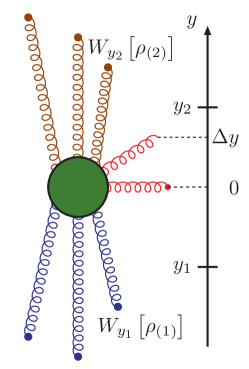
Figure 1: Production of two gluons: the integral over $\Delta y$ is divergent.

In the fully nonlinear case of AA collisions the $k_{T}$-factorization is broken (see e.g. [5, 16]), and one must solve the equations of motion to all orders in the strong classical field. The analogue of the unintegrated parton distributions $\varphi_{y}({\boldsymbol{k}_{\perp}})$ is the color charge density distribution $W_{y}[\rho]$. These are similar in the sense that they are not (complex) wavefunctions but (at least loosely speaking) real probability distributions. Factorization can be understood as a statement that one has found a convenient set of degrees of freedom in which one can compute physical observable from only the diagonal elements of the density matrix of the incoming nuclei. The difference is that when in the dilute case these degrees of freedom are numbers of gluons with a given momentum, in the nonlinear case the appropriate variable is the color charge density and the relevant evolution equation is JIMWLK, not BFKL. The kinematical situation, however, remains the same. To produce a gluon at a very large rapidity (or a contribution in the loop integral of the virtual contribution with a large $k^{+}$) one must get a large $+$-momentum from the right-moving source. Thus one is probing the source at a large $k^{+}$, i.e. small distances in $x^{-}$, and the result must involve $W_{y}[\rho]$ at a larger rapidity. The underlying physical interpretation of factorization is that this fluctuation with a large $k^{+}$ requires such a long interval in $x^{+}$ to radiated that it must be produced well before and independently of the interaction with the other (left moving and thus localized in $x^{+}$) source. The concrete task is then to show that when one computes the NLO corrections to a given observable in the Glasma, all the leading logarithmic divergences can be absorbed into the RG evolution of the sources with the same Hamiltonian that was derived by considering only the DIS process. This is the proof [11, 12, 17] of factorization that we will briefly describe in the following.

3 Deriving JIMWLK factorization

Consider the single inclusive gluon multiplicity which is a sum of probabilities to produce $n+1$ particles, with the phase space of the additional $n$ must be integrated out

$$\frac{dN}{d^{3}\vec{\boldsymbol{p}}}\sim\sum_{n=0}^{\infty}\frac{1}{n!}\int\Big{[}d^{3}\vec{\boldsymbol{p}}_{1}\cdots d^{3}\vec{\boldsymbol{p}}_{n}\Big{]}\;\left|\big{<}{\vec{\boldsymbol{p}}}\;\,\vec{\boldsymbol{p}}_{1}\cdots\vec{\boldsymbol{p}}_{n}\big{|}0\big{>}\right|^{2}.$$ (3)

Because we have a theory with external color sources of order $\rho\sim 1/g,$ all insertions of source appear at the same order [18]. A calculation using the Schwinger-Keldysh formalism leads to the following results: At LO, the multiplicity is obtained from the retarded solution of classical field equations (here $(\dots)$ includes the appropriate normalization and projection to physical polarizations)

$$\frac{\mathrm{d}N_{{}_{\rm LO}}}{d^{3}\vec{\boldsymbol{p}}}=\!\int\!\mathrm{d}^{3}{\boldsymbol{x}}\mathrm{d}^{3}{\boldsymbol{y}}\;e^{i\vec{\boldsymbol{p}}\cdot(\vec{\boldsymbol{x}}-\vec{\boldsymbol{y}})}\;(\cdots)\Big{[}{{\cal A}^{\mu}(t,\vec{\boldsymbol{x}})}{{\cal A}^{\nu}(t,\vec{\boldsymbol{y}})}\Big{]}\Big{|}_{t\to\infty}.$$ (4)

The NLO contribution includes the one loop correction to the classical field and the $+-$ component of the Schwinger-Keldysh (SK) propagator in the background field

$$\frac{\mathrm{d}N_{{}_{\rm NLO}}}{d^{3}\vec{\boldsymbol{p}}}\!\!=\!\int_{{\boldsymbol{x}},{\boldsymbol{y}}}\!\!\!\;e^{i\vec{\boldsymbol{p}}\cdot(\vec{\boldsymbol{x}}-\vec{\boldsymbol{y}})}\;(\cdots)\Big{[}{\mathcal{G}_{+-}^{\mu\nu}(x,y)}+{\beta_{+}^{\mu}(t,\vec{\boldsymbol{x}})}\;{\mathcal{A}_{-}^{\nu}(t,\vec{\boldsymbol{y}})}+{\mathcal{A}_{+}^{\mu}(t,\vec{\boldsymbol{x}})}\;{\beta_{-}^{\nu}(t,\vec{\boldsymbol{y}})}\Big{]}\Big{|}_{t\to\infty}.$$ (5)

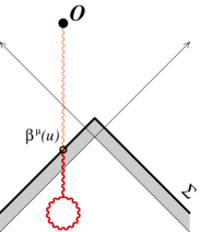
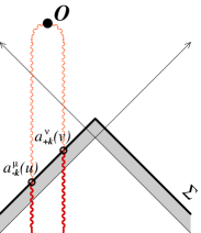
Figure 2: The 1-loop one and two point functions in the background field.

Because of the SK index structure (also $\beta$ satisfies an equation of motion with a retarded boundary condition), one can express the propagation of a small fluctuation $a^{\mu}(x)$ above the past light cone $\Sigma$ as a functional derivative $\mathbb{T}_{{\boldsymbol{u}}}$ of the LO classical field $\mathcal{A}^{\mu}(x)$ with respect to its initial condition on $\Sigma$: $a^{\mu}(x)=\int_{\vec{\boldsymbol{u}}\in{\rm\Sigma}}a(\vec{\boldsymbol{u}})\cdot\mathbb{T}_{{\boldsymbol{u}}}\mathcal{A}^{\mu}(x).$ This leads after some rearrangements to the expression for the NLO contribution to the multiplicity as a functional derivative operator acting on the leading order result:

$$\left.\frac{dN}{d^{3}\vec{\boldsymbol{p}}}\right|_{{}_{\rm NLO}}=\bigg{[}\frac{1}{2}\!\int_{\Sigma}\!\mathrm{d}^{3}{\boldsymbol{u}}\mathrm{d}^{3}{\boldsymbol{v}}\mathcal{G}_{\mu\nu}({\boldsymbol{u}},{\boldsymbol{v}})\mathbb{T}^{\mu}_{{\boldsymbol{u}}}\mathbb{T}^{\nu}_{{\boldsymbol{v}}}+\int_{\Sigma}\!\mathrm{d}^{3}{\boldsymbol{u}}\mathbf{\beta}_{\mu}({\boldsymbol{u}})\mathbb{T}^{\nu}_{{\boldsymbol{u}}}\bigg{]}\;\left.\frac{dN}{d^{3}\vec{\boldsymbol{p}}}\right|_{{}_{\rm LO}}.$$ (6)

Here the two point function below the light cone $\mathcal{G}^{\mu\nu}(\vec{\boldsymbol{u}},\vec{\boldsymbol{v}})\equiv\int\frac{d^{3}\vec{\boldsymbol{k}}}{(2\pi)^{3}2E_{\boldsymbol{k}}}\;a^{\mu}_{-{\boldsymbol{k}}}({\boldsymbol{u}})\,a^{\nu}_{+{\boldsymbol{k}}}({\boldsymbol{v}})$ is bilinear in the small fluctuation field $a^{\mu}(x)$ satisfying the small fluctuation equation of motion with and initial condition given by a plane wave $\lim_{x^{0}\to-\infty}a^{\mu}_{\pm{\boldsymbol{k}}}(x)=\epsilon^{\mu}({\boldsymbol{k}})e^{\pm ik\cdot x}$; see Fig. 2 for a pictorial representation of this structure.

The leading logarithmic contribution comes from the longitudinal component of the integral over ${\boldsymbol{k}}$, the momentum of the initial plane wave perturbation (and the corresponding momentum in the one loop source term for the equation of motion satisfied by $\beta$). This LLog part of the functional derivative (6) operator turns out to be precisely equivalent to the sum of the JIMWLK Hamiltonians describing the RG evolution of the source distributions $W_{y}[\rho]$. The fact that no other terms with the same logarithmic divergences appear is the crucial result for factorization. The JIMWLK Hamiltonian

$$\mathcal{H}\equiv\frac{1}{2}\int\!\mathrm{d}^{2}{\boldsymbol{x}_{\perp}}\mathrm{d}^{2}{\boldsymbol{y}_{\perp}}D_{a}({\boldsymbol{x}_{\perp}})\eta^{ab}({\boldsymbol{x}_{\perp}},{\boldsymbol{y}_{\perp}})D_{b}({\boldsymbol{y}_{\perp}})$$ (7)

is most naturally expressed in terms of Lie derivatives $D_{a}({\boldsymbol{x}_{\perp}})$ operating on the Wilson lines formed from the classical field ($U({\boldsymbol{x}_{\perp}})=\mathrm{P}\exp\left\{-ig\int\mathrm{d}x^{-}\left(1/\boldsymbol{\nabla}_{\perp}^{2}\right)\rho({\boldsymbol{x}_{\perp}},x^{-})\right\}$ for the nucleus moving in the $+z$ direction) in terms of which the kernel in Eq. (7) is

$$\eta^{ab}({\boldsymbol{x}_{\perp}},{\boldsymbol{y}_{\perp}})=\frac{1}{\pi}\int_{{\boldsymbol{u}_{\perp}}}\!\!\frac{({\boldsymbol{x}_{\perp}}-{\boldsymbol{u}_{\perp}})\cdot({\boldsymbol{y}_{\perp}}-{\boldsymbol{u}_{\perp}})}{({\boldsymbol{x}_{\perp}}-{\boldsymbol{u}_{\perp}})^{2}({\boldsymbol{y}_{\perp}}-{\boldsymbol{u}_{\perp}})^{2}}\;\Big{[}U_{\boldsymbol{x}_{\perp}}U^{\dagger}_{\boldsymbol{y}_{\perp}}-U_{\boldsymbol{x}_{\perp}}U^{\dagger}_{\boldsymbol{u}_{\perp}}-U_{\boldsymbol{u}_{\perp}}U^{\dagger}_{\boldsymbol{y}_{\perp}}+1\Big{]}^{ab}.$$ (8)

Let us conclude by summarizing some important aspects of the JIMWLK factorization theorem of Refs. [11, 12]. We are interested in the high energy kinematical limit, with transverse momenta $\sim Q_{\mathrm{s}}$ and the energy $s$ large; the dilute limit is that of BFKL physics. The relevant degrees of freedom in this framework are the color charge densities $\rho$ of the fast partons and the classical fields of the small $x$ ones. The color charges $\rho\sim 1/g$ are parametrically large, and thus the problem is inherently nonperturbative, but there is, however, a consistent weak coupling or loop expansion. The primary observables of interest are inclusive single and multigluon multiplicities (not cross sections for producing a fixed number of particles), which leads to results that can be expressed in terms of retarded (and advanced) propagators. We express these propagators as functional derivatives with respect to the field on an initial surface on the light cone, which can then be mapped to the functional derivatives of the color fields of the individual nuclei appearing in the JIMWLK Hamiltonian.

Acknowledgments: R. V.’s work is supported by the US Department of Energy under DOE Contract No. DE-AC02-98CH10886. F.G.’s work is supported in part by Agence Nationale de la Recherche via the programme ANR-06-BLAN-0285-01.

References

- [1] E. Iancu and R. Venugopalan, arXiv:hep-ph/0303204.
- [2] H. Weigert, Prog. Part. Nucl. Phys. 55, 461 (2005), [arXiv:hep-ph/0501087].
- [3] L. D. McLerran and R. Venugopalan, Phys. Rev. D49, 2233 (1994), [arXiv:hep-ph/9309289].
- [4] T. Lappi and L. McLerran, Nucl. Phys. A772, 200 (2006), [arXiv:hep-ph/0602189].
- [5] A. Krasnitz and R. Venugopalan, Nucl. Phys. B557, 237 (1999), [arXiv:hep-ph/9809433].
- [6] A. Krasnitz, Y. Nara and R. Venugopalan, Phys. Rev. Lett. 87, 192302 (2001), [arXiv:hep-ph/0108092].
- [7] T. Lappi, Phys. Rev. C67, 054903 (2003), [arXiv:hep-ph/0303076].
- [8] F. Gelis and R. Venugopalan, Phys. Rev. D69, 014019 (2004), [arXiv:hep-ph/0310090].
- [9] F. Gelis, K. Kajantie and T. Lappi, Phys. Rev. C71, 024904 (2005), [arXiv:hep-ph/0409058].
- [10] F. Gelis, K. Kajantie and T. Lappi, Phys. Rev. Lett. 96, 032304 (2006), [arXiv:hep-ph/0508229].
- [11] F. Gelis, T. Lappi and R. Venugopalan, Phys. Rev. D78, 054019 (2008), [arXiv:0804.2630 [hep-ph]].
- [12] F. Gelis, T. Lappi and R. Venugopalan, Phys. Rev. D78, 054020 (2008), [arXiv:0807.1306 [hep-ph]].
- [13] L. V. Gribov, E. M. Levin and M. G. Ryskin, Phys. Rept. 100, 1 (1983).
- [14] D. Kharzeev, Y. V. Kovchegov and K. Tuchin, Phys. Rev. D68, 094013 (2003), [arXiv:hep-ph/0307037].
- [15] A. Leonidov and D. Ostrovsky, Phys. Rev. D62, 094009 (2000), [arXiv:hep-ph/9905496].
- [16] J.-P. Blaizot and Y. Mehtar-Tani, arXiv:0806.1422 [hep-ph].
- [17] F. Gelis, T. Lappi and R. Venugopalan, Int. J. Mod. Phys. E16, 2595 (2007), [arXiv:0708.0047 [hep-ph]].
- [18] F. Gelis and R. Venugopalan, Nucl. Phys. A776, 135 (2006), [arXiv:hep-ph/0601209].