Atomistic spin dynamics of the CuMn spin glass alloy

Abstract

We demonstrate the use of Langevin spin dynamics for studying dynamical properties of an archetypical spin glass system. Simulations are performed on CuMn (20% Mn) where we study the relaxation that follows a sudden quench of the system to the low temperature phase. The system is modeled by a Heisenberg Hamiltonian where the Heisenberg interaction parameters are calculated by means of first-principles density functional theory. Simulations are performed by numerically solving the Langevin equations of motion for the atomic spins. It is shown that dynamics is governed, to a large degree, by the damping parameter in the equations of motion and the system size. For large damping and large system sizes we observe the typical aging regime.

I Introduction

Spin glasses exhibit exotic dynamical properties such as aging, memory, and rejuvenation, which have triggered a lot of research in the past.Binder and Young (1986); Young (1998) The interest in dynamics in these systems is mainly motivated by the fact that practically only off-equilibrium properties of spin glasses can be observed in experiments. Peculiarities in the dynamical behavior are often related to a complex nature of the phase space and the lack of ergodicity in spin-glass systems.Palmer (1982) In particular, relaxation towards equilibrium is not characterized by a single timescale but rather by a broad spectrum of relaxation times leading to a non-trivial evolution of measurable quantities, like e.g. magnetization.

An aging experiment is an elegant way to reveal the multiscale nature of the spin-glass dynamics. Lundgren et al. (1983) A system is prepared by quenching from a high temperature to a given temperature $T$ and perturbing the system in some way, usually by switching on an external magnetic field. A measurement of the time evolution of the magnetization is performed after a certain time, $t_{w}$, has passed since the system preparation. For temperatures $T$ below the spin-glass transition temperature $T_{g}$, relaxation of the magnetization towards the equilibrium value shows a strong dependence on the waiting time, $t_{w}$. A number of phenomenological models has been proposed to explain this behavior, among which are the well-known droplet model Fisher and Huse (1988) and a class of hierarchial models. Ogielski and Stein (1985); Teitel and Domany (1985); Huberman and Kerszberg (1985); Sibani and Hoffmann (1989); Bouchaud and Dean (1995) However, scaling laws resulting from these models does not allow to interpret experimental results unambiguously, since this would require the access to asymptotic regimes of relaxation and hence enormously large time scales. Moreover, different, sometimes even contradicting, models give rise to same scaling laws, discrediting their predictions. Studying realistic models seems therefore to be a more promising way to elucidate mechanisms underlying spin-glass dynamics.

There has been much work on the non-equilibrium behavior of Edward-Anderson (EA) spin-glass models. Andersson et al. (1992); Ozeki and Ito (2001); Katzgraber and Campbell (2005); Blundell et al. (1992); Ogielski (1985); Picco et al. (2001); Rieger (1993); Berthier and Bouchaud (2002) These numerical studies have shown that the dynamical behavior of the correlation function is very similar to that of the magnetization (related to the correlation function via the fluctuation-dissipation theorem in equilibrium) in experiments. In particular, the two-stage relaxation depending on the waiting time is reproduced in the simulations.

In this paper, we study the spin-glass dynamics of the Cu₈₀Mn₂₀ alloy by modeling it with the random-site Heisenberg Hamiltonian:

$$\mathscr{H}=-\sum_{i,j}J_{ij}c_{i}c_{j}\textbf{m}_{i}\cdot\textbf{m}_{j},$$ (1)

where $\textbf{m}_{i}$ represent vector magnetic moments and $c_{i}$ are the occupation numbers of the magnetic atoms ($c_{i}$ is equal to 1 if a site is occupied by a Mn atom and 0 otherwise); exchange parameters $J_{ij}$ are calculated accurately within the density function theory (DFT) approach. Usually, dynamics of spin glasses is studied by means of Monte-Carlo simulations. Berthier and Bouchaud (2002); Blundell et al. (1992); Rieger (1993); Katzgraber and Campbell (2005); Kisker et al. (1996); Ogielski (1985) Such an approach misses some details of local relaxations of spins in their local fields. The influence of the finite rate of these local relaxations on the dynamics in general can be investigated by solving the Langevin dynamics equations directly. As a matter of fact, as will be shown below, motion of individual spins can have a rather strong impact on the aging behavior of the system.

In the next section, we introduce definitions used throughout the paper and describe briefly the way aging is observed in experiments. In Section III, governing equations for the atomistic spin dynamics are given along with some details on the implementation. Results of the numerical simulations of the CuMn alloy and EA model are presented in Section IV. The focus is on the influence of damping on the spin dynamics.

II Definitions and Theory

In a typical aging experiment, a system is quenched in zero field from high temperature to a temperature below $T_{g}$. Then the system is aged during a waiting time $t_{w}$, a small constant field $h$ is applied and the time dependence of the magnetization $M(t)$ or susceptibility $\chi(t)=M(t)/h$ is observed. The relaxation process after the quench can be associated with three phases: (1) an initial relaxation towards a local quasi-equilibrium state, (2) aging dynamics and (3) global equilibration. The latter is achievable only for systems of finite size $N$ within a time greater than the ergodic time $\tau_{erg}\sim\exp{(N)}$. Although equilibration is of little interest in an experiment, it must be taken into account in numerical simulations when one deals with relatively small systems.

In numerical simulations, it is convenient to work with the autocorrelation function:

$$C(t_{w}+t,t_{w})=\frac{1}{N}\sum_{i}\left[\textbf{m}_{i}(t_{w})\cdot\textbf{m}_{i}(t_{w}+t)\right]_{\textrm{av}},$$ (2)

where $[\dots]_{\textrm{av}}$ stand for configuration averaging, i.e. averaging over independent runs with randomly generated atomic distributions $\{c_{i}\}$. In the quasi-equilibrium phase, when the conditions for the fluctuation-dissipation theorem (FDT) are fulfilled, the autocorrelation is related to the response function Young (1998):

$$R(t_{w}+t,t_{w})=-\frac{1}{T}\frac{\partial C(t_{w}+t,t_{w})}{\partial t_{w}}.$$ (3)

Within linear response, the (thermoremanent) magnetization and susceptibility can be found in the following way:

$$M(t_{w}+t,t_{w}) = h\int_{0}^{t_{w}}dt^{\prime}R(t_{w}+t,t^{\prime}),$$ (4)

$$\chi(\omega,t_{w}) = \int_{0}^{t_{w}}dt^{\prime}R(t_{w},t^{\prime})e^{i\omega(t^{\prime}-t_{w})},$$ (5)

where $h$ is a small applied magnetic field in a corresponding thermoremanent magnetization (TRM) experiment. In quasi-equilibrium, the relaxation of observables does not depend on $t_{w}$ and the relation between the magnetization and the autocorrelation function amounts to

$$M(t)=M_{0}-\frac{h}{T}C_{\mathrm{eq}}(t),$$ (6)

where $C_{\mathrm{eq}}(t)\equiv C(t_{w}+t,t_{w})$ in a $t_{w}$-independent regime. In a non-equilibrium situation, when the FDT is violated, different stages of the autocorrelation relaxation can be illustrated by the relaxation rate function defined as

$$S(t_{w}+t,t_{w})=-\frac{d}{d\ln{t}}C(t_{w}+t,t_{w}).$$ (7)

The relaxation rate peaks at a time $t_{a}$ of the order of the age of the system, i.e. $t_{a}\sim t_{w}$.

Spin dynamics of a spin glass is essentially non-equilibrium, and the aging behavior in particular makes the evolution of the autocorrelation function be strongly dependent on the waiting time, i.e. time-translation invariance is violated. However, under certain circumstances or during certain time intervals, a condition of time-translation invariance, $C(t_{w}+t,t_{w})=C(t)$, holds and the relaxation of the system is said to proceed in the quasi-equilibrium regime. This assertion can be considered as a definition of a quasi-equilibrium state. In order for the true equilibrium dynamics to take place, the fluctuation-dissipation theorem must hold.

Having been prepared at a temperature $T$, the system tends to the equilibrium state. This state can be characterized by the space correlation function which for spin-glasses is calculated in the following way:

$$G(R)=\frac{1}{N}\sum_{i}\left[(\langle\mathbf{m}_{i}\cdot\mathbf{m}_{i+R}\rangle-\langle\mathbf{m}_{i}\rangle\cdot\langle\mathbf{m}_{i+R}\rangle)^{2}\right]_{\textrm{av}}.$$ (8)

Above the transition temperature for sufficiently large $R$, the spatial correlation is given by

$$G(R)\sim R^{d-2+\eta}u(R/\xi),$$ (9)

where $d$ is the dimension of the system, $\eta$ a critical exponent, $\xi$ the correlation length and $u(x)$ a scaling function which decays to zero for $R/\xi\rightarrow\infty$. In the macroscopic limit, the correlation length $\xi$ is finite above $T_{g}$ but diverges with $\xi\sim\epsilon^{-\nu}$ as $T_{g}$ is approached from above, where $\epsilon=(T-T_{g})/T_{g}$ is the reduced temperature and $\nu$ is a critical exponent.

III Description of method

Our simulations are performed using the ASD (Atomic Spin Dynamics) packageSkubic et al. (2008) which is based on an atomistic approach for spin dynamics. We use a parametrization of the interatomic exchange part of the Hamiltonian in the form of Eq. 1. The effect of temperature is modeled by Langevin dynamics. Connection to an external thermal bath is modeled with a Gilbert-like damping characterized by a damping parameter $\alpha$.

The microscopic equations of motion for the atomic moments, $\mathbf{m}_{i}$, in an effective field, $\mathbf{B}_{i}$, are expressed as follows:

$$\frac{d\mathbf{m}_{i}}{dt}=-\gamma\mathbf{m}_{i}\times[\mathbf{B}_{i}+\mathbf{b}_{i}(t)]-\gamma\frac{\alpha}{m}\mathbf{m}_{i}\times(\mathbf{m}_{i}\times[\mathbf{B}_{i}+\mathbf{b}_{i}(t)]).$$ (10)

In this expression $\gamma$ is the electron gyromagnetic ratio and $\mathbf{b}_{i}(t)$ is a stochastic magnetic field with a Gaussian distribution. The magnitude of that field is related to the damping parameter, $\alpha$, in order for the system to eventually reach thermal equilibrium.

The effective field, $\mathbf{B}_{i}$, on a site $\it i$, is calculated from

$$\mathbf{B}_{i}=-\frac{\partial\mathscr{H}}{\partial\mathbf{m}_{i}},$$ (11)

where for $\mathscr{H}$ we use the classical Heisenberg Hamiltonian defined by Eq. 1.

We use Heuns method (for details see Ref. Skubic et al., 2008) with a time step size of 0.01 femtoseconds for solving the stochastic differential equations. Most of the calculations are performed up to a time $t=70\mathrm{ps}$.

IV Langevin spin dynamics of a Heisenberg spin glass

IV.1 Spin dynamics of CuMn

Spin dynamics simulations are performed for the CuMn alloy with 20% of magnetic atoms (Mn). The system is described by the Heisenberg Hamiltonian with spins (magnetic atoms) distributed over the fcc lattice. The magnetic exchange (for the Heisenberg Hamiltonian) parameters are obtained by means of the screened generalized perturbation method (SGPM)Ruban et al. (2004) implemented within the exact muffin-tin orbital (EMTO)Vitos (2001) scheme. The coherent potential approximation (CPA) and disordered local moments (DLM) are used to treat the disordered CuMn alloy in the paramagnetic state properly. With this model and for 20 % Mn, critical slowing down occurs close to the experimental freezing temperature, $T_{g}$, which is approximately 90 K.Gibbs et al. (1985) In contrast to the EA model, where bonds between atomic spins are random and the atomic sites ordered, for CuMn, the magnetic exchange parameters between the Mn atoms are site-independent and the atomic sites for these atoms are randomly distributed in the lattice. Simulations are performed on a $32\times 32\times 32$ fcc system with 20 % of the atomic sites occupied by Mn. We simulate the relaxation process following a quench from completely random spin orientations to 10 K. Averaging is performed over 10 random alloy configurations with fixed interatomic exchange parameters.

The main concern of the current work is to investigate the influence of damping on the aging behavior and on spin relaxation in general, motivation being that the damping parameter is the only parameter of the model not derived from first principles calculations.

First, it is worth considering two limiting cases: $\alpha=0$ and $\alpha=\infty$. The first case is trivial and corresponds to an utterly deterministic evolution with the total energy conserved. We can call this a ”microcanonical dynamics” for brevity. Since there is no coupling to a heat bath, the system will never reach equilibrium in this type of dynamics. In case of the infinite damping parameter, on the other hand, relaxation of a spin to equilibrium with respect to its local magnetic field occurs instantaneously, and spin dynamics becomes equivalent to the dynamics of the heat-bath Monte Carlo method.Olive et al. (1986) For intermediate values of the damping parameter, we expect a system to cross over from the initial off-equilibrium dynamics to the regime of relaxation towards a (quasi-) equilibrium state. The duration of the crossover must be dependent on the damping parameter.

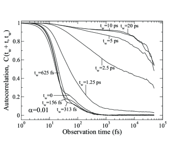
Figure 1: Autocorrelation $C(t_{w}+t,t_{w})$ calculated for CuMn after a quench from completely random spin orientations to T=10 K with damping $\alpha=0.01$. The autocorrelation is presented (from left to right in the figure) for the logarithmically spaced waiting times $t_{w}=0$, $1.56\cdot 10^{2}$, $3.13\cdot 10^{2}$, $6.25\cdot 10^{2}$, $1.25\cdot 10^{3}$, $2.5\cdot 10^{3}$, $5\cdot 10^{3}$, $1\cdot 10^{4}$, and $2\cdot 10^{4}$ fs.

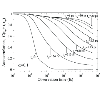
Figure 2: Same as Fig. 1 but with damping $\alpha=0.0316$.

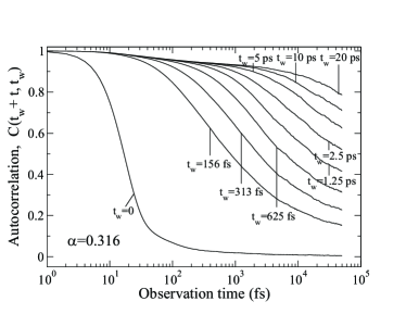
Figure 3: Same as Fig. 1 but with damping $\alpha=0.1$.

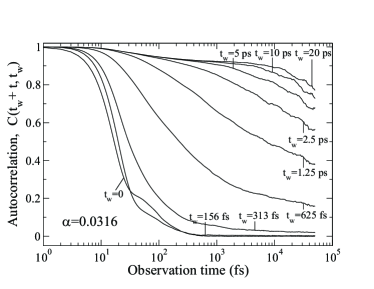
Figure 4: Same as Fig. 1 but with damping $\alpha=0.316$.

In Figs. 1-4 we show the spin glass dynamics of CuMn for four different damping parameters, $\alpha=0.01,0.0316,0.1,0.316$ respectively. We plot the autocorrelation function for logarithmically spaced waiting times. Note that the time is given in femtoseconds, but the time step size in the simulation is 0.01 fs. In all four cases, the autocorrelation for $t_{w}$=0 illustrates the initial dynamics of the system right after the quench. The behavior at short times ($t\lesssim 500$ fs) is similar for all values of $\alpha$ and is shown in Fig. 5 in log-linear scale. The evolution of the autocorrelation function can be described here as a sum of two exponents followed by a slower-than-exponential decay at larger times. That is for $t\lesssim 200$ fs, we have

$$C(t,0)\approx(1-A)e^{-\frac{t}{\tau_{1}}}+Ae^{-\frac{t}{\tau_{2}}},$$ (12)

where $A$ can be extracted from the the intersection point of straight lines corresponding to the second exponent: $A=0.32\pm 0.02$. The bump in Figs. 1-4 on the curves for $t_{w}=0$ corresponds to the second term in Eq. 12. The initial slope of the curves, $1/\tau_{1}$, is independent of damping (see Fig. 5) and temperature (data not shown) and depends only on the details of the Hamiltonian and initial spin distribution. When the initial distribution is random, as is the case in present simulations, the drop of the autocorrelation is dominated by the strong precessional motion of the atomic spins in rapidly varying effective exchange fields. As the directions of the effective fields initially are completely randomly oriented, the angle between the atomic spin and its effective field is on average large, resulting in a large precessional torque on the atomic spins. The system gradually relaxes by means of a damping torque on each atomic spin, with the energy of the system dropping down from a high value of the random spin configuration (”high-temperature” phase) to a value close to the average energy for $T=10K$.

The subsequent decay of the autocorrelation is associated with the equilibration of spins in their local fields. Clearly, the rate of this relaxation, $1/\tau_{2}$, depends strongly on the value of the damping parameter and for this reason we refer to it as ”damping relaxation”. As the rate $1/\tau_{2}$ diminishes with increasing $\alpha$, the initial damping relaxation becomes more difficult to identify. As it is seen in Fig. 5 for $\alpha=0.316$, the crossover from the initial stage to non-exponential decay is rather smooth and relaxation due to damping is indistinguishable.

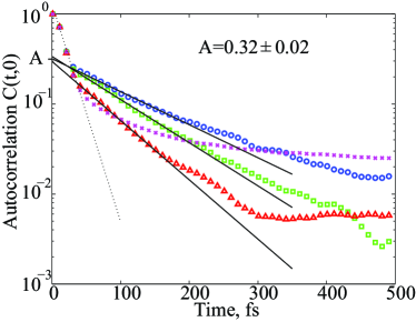
Figure 5: Autocorrelation $C(t,t_{w}=0)$ for four values of the damping parameter: $\alpha=0.01$ (circles), $\alpha=0.0316$ (boxes), $\alpha=0.1$ (triangles), $\alpha=0.316$ (crosses). The dashed line is a linear fit to the points for 10 fs$\leq t\leq$ 40 fs; the slope is equal to $1/\tau_{1}$ of Eq. 12. The slope of the solid lines corresponds to the damping relaxation rate $1/\tau_{2}$ in Eq. 12.

The rate of the damping relaxation affects the behavior of the autocorrelation function for waiting times much larger than the value of $\tau_{2}$. From Fig. 1 one can see that for $\alpha=0.01$, the curves fall on top of each other for waiting times up to $t_{w}=625$ fs. This implies that by this moment, the decay of the autocorrelation function has become time-translation invariant. In fact, it seems that for this value of the damping parameter, the system never enters the aging regime and the initial relaxation phase crosses over directly to relaxation to the global equilibrium for $t_{w}>5$ fs. On the other hand, at smaller values of $\tau_{2}$, the aging behavior recovers (see Figs. 3,4) and the spin dynamics is similar to the case of infinite damping. This implies that the strength of damping is determined by the the ratio of the timescale $\tau_{2}$ of the damping relaxation and the characteristic time of detuning of local fields due to the motion of neighboring spins contributing to these local fields.

To determine to what extent the system has equilibrated, one can look at the evolution of the spin-spin correlation function $g(\mathbf{r}_{ij})=\langle\mathbf{m}_{i}\cdot\mathbf{m}_{j}\rangle$. In Fig. 6 we plot $g(\mathbf{r}_{ij})$ as a function of the distance $|\mathbf{r}_{ij}|$ between the spins for different waiting times of the system. The correlation function is plotted both for $\alpha=0.01$ (upper panel) and $\alpha=0.1$ (lower panel). As expected from the autocorrelation, $g(\mathbf{r}_{ij})$ is seen to evolve faster for the larger damping. It means that for sufficiently large damping the system reaches the quasi-equilibrium phase fast enough for the aging regime to establish.

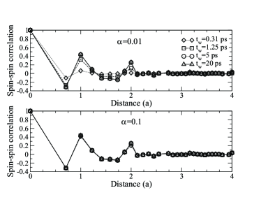
Figure 6: The calculated spin-spin correlation function,$\langle\mathbf{m}_{i}\cdot\mathbf{m}_{j}\rangle$, for $\alpha=0.01$ (upper panel) and $\alpha=0.1$ (lower panel). The correlation function is plotted for four logarithmically spaced waiting times. For $\alpha=0.1$, all four curves fall essentially on top of each other.

The non-equilibrium behavior seen at small waiting times for small damping parameter values can be detected on the microscopic level by observing the trajectories of randomly selected spins. In Fig. 7 we plot the trajectory of a typical atomic spin evolving during 100 fs (corresponding to a short time scale), for $\alpha=0.01$ and $\alpha=0.1$, and for two different waiting times. The upper panel shows a trajectory for $\alpha=0.01$ after a waiting time of 1.25 ps. There is a large degree of precessional motion of the atomic spin, confirming the conclusions which were drawn from the autocorrelation that the system is still in the initial relaxation phase at this waiting time. The middle panel shows the same system after a waiting time of 5 ps, showing an atomic spin with a much more stable spin direction. The spin is now either in equilibrium or on the verge of entering equilibrium, although spin motion is much more pronounced here than in the aging regime for the system with $\alpha=0.1$. The lower panel shows the trajectory of an atomic spin for $\alpha=0.1$ at a waiting time of 1.25 ps. The system is here in the aging regime, as seen in Fig. 2, and the atomic spin direction is stable on a time scale of 100 fs.

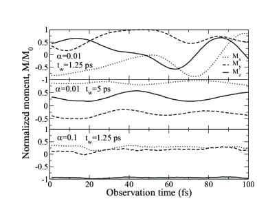
Figure 7: The trajectory for one typical atomic spin at $t_{w}=1.25$ ps for $\alpha=0.01$ (upper panel), at $t_{w}=5$ ps for $\alpha=0.01$ (middle panel) and at $t_{w}=1.25$ ps for $\alpha=0.1$ (lower panel).

In the aging regime, the autocorrelation is characterized by an initial reduction of the autocorrelation on to a plateau, similar to what is seen for systems in equilibrium. A plateau is clearly seen in Figs. 1-4 for larger waiting times. The position of the plateau depends on temperature and is related to the spin-glass order parameter. More precisely,

$$\lim_{t\to\infty}\lim_{t_{w}\to\infty}C(t_{w}+t,t_{w})=q_{\mathrm{EA}}$$ (13)

in the macroscopic limit, and the Edward-Anderson order parameter, $q_{\mathrm{EA}}$, is defined (again in the macroscopic limit) as

$$q_{\mathrm{EA}}=\frac{1}{N}\sum_{i}\left[\langle\mathbf{m}_{i}\rangle^{2}_{T}\right]_{\mathrm{av}},$$ (14)

where $\langle\dots\rangle_{T}$ is thermal averaging. Following the plateau, or the quasi-equilibrium phase, is the aging phase. The crossover from one phase to another occurs at a time, $t_{s}$, when a sudden drop of the autocorrelation takes place. The time $t_{s}$ can be best identified as the maximum of the relaxation rate defined by Eq. 7.

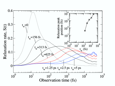
Figure 8: Relaxation rate, $S(t)$, for the simulation in Fig. 3. The relaxation rate is plotted for the logarithmically spaced waiting times $t_{w}=0$, $1.56\cdot 10^{2}$, $3.13\cdot 10^{2}$, $6.25\cdot 10^{2}$, $1.25\cdot 10^{3}$, $2.5\cdot 10^{3}$, and $5\cdot 10^{3}$ fs. The inset shows the relationship between the waiting time and the peak of the relaxation rate for the waiting times $t_{w}=1.56\cdot 10^{2}$, $3.13\cdot 10^{2}$, $6.25\cdot 10^{2}$, $1.25\cdot 10^{3}$, and $2.5\cdot 10^{3}$ fs. For the last waiting time the largest peak seems to be a numerical artifact. Instead the second largest peak was chosen as input for the inset.

The relaxation rate for $\alpha=0.1$ and for a few waiting times is plotted in Fig. 8. The relaxation rate is calculated by performing a derivative with respect to $\ln{t}$ of the autocorrelation. Note that, the poorly defined peaks at the end of the observation time ($t\sim 10^{4}$ fs) are artifacts of a smearing scheme, used when calculating the derivative and which breaks down close to the edge of the observation interval. In the inset we show the position of the peak relaxation rate, or $t_{s}$, with respect to the waiting time. As one can see, $t_{s}$ is slightly larger than $t_{w}$, which is expected for the aging regime in a spin-glass system. Zotev et al. (2003) However, the total time window used in the simulations does not allow to infer any definite form of the dependence.

IV.2 Spin dynamics of the EA model for weak damping

To investigate even further spin dynamics for small $\alpha$, we have performed simulations of the EA model for $\alpha=0.01$ and for different lattice sizes. Simulations have been performed on a cubic lattice of different sizes $L\times L\times L$, where $L$=4, 8, 16, and with random nearest neighbor exchange interactions drawn from a Gaussian distribution with a standard deviation of 1 mRy. This is typically the order of the exchange interaction. The freezing temperature, $T_{g}$, is expected to be 25 K for this model (0.16 within the dimensionless model).Berthier and Young (2004)

In Fig. 9, we show the calculated autocorrelation for a simulation of the Edwards-Anderson model. The simulated process is a relaxation following a quench from completely random spin orientations to 10 K (0.063 within the standard dimensionless model). The autocorrelation with respect to observation time is plotted for several logarithmically spaced waiting times. As in the case of the CuMn simulations, averaging was performed over 10 different bond realizations, and for each bond configuration, 10 simulations with different initial random spin distributions and different random number sequences in the Langevin equations have been done.

There are three sets of curves in Fig. 9 for three different system sizes. As it is seen, for the choice of the damping parameter ($\alpha=0.01$) and system sizes ($L=4,8,16$), the aging regime is very short or even non-present in these simulations. A global equilibrium is reached very soon after the initial relaxation has been accomplished. It is also worth noting that with the same damping parameter, there is a strong similarity between the waiting time dependence of the auto correlation function for the 16$\times$16$\times$16 EA model (Fig. 9 ) and the dilute 20$\times$20$\times$20 CuMn alloy (Fig. 1). Moreover, comparing the curves corresponding to the initial phase ($t_{w}=0$), one can see that this initial phase is independent of the system size.

Typically, a spin glass system enters the aging regime as soon as local equilibrium conditions are being met. The dynamics proceeds by a rearrangement of the magnetic order on a length scale corresponding to a time scale of the order of the age of the system. In this particular simulation, a pure aging regime can not be identified as the system enters a global equilibrium soon after the initial relaxation. In contrast to equilibrium, within the aging regime, the autocorrelation should depend on the waiting time and not on the system size. For the largest four waiting times in Fig. 9, we see the autocorrelation characterized by an initial reduction on to a plateau followed by a large sudden reduction to zero for different observation times depending on the size of the system.

A global equilibrium is reached for finite systems, as the correlation length reaches the size of the system. If there is aging dynamics, it can no longer proceed. In equilibrium, thermal fluctuations continue to govern the motion of the atomic spins. Since there is no energy associated with a global rotation of the system, the autocorrelation is reduced to zero in equilibrium. The autocorrelation is now translationally invariant with respect to the observation time, $t$. By comparing simulations on systems of different size we see that by increasing the size of the system by a factor 2, the equilibration time is increased approximately by a factor $3$. This is due to the fact that the correlation length grows logarithmically in time.

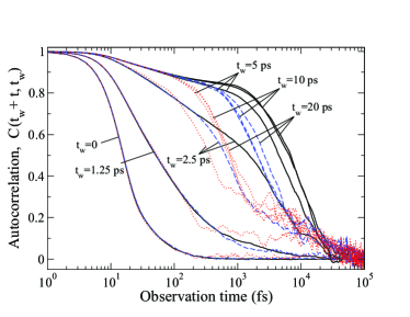
Figure 9: Autocorrelation $C(t_{w}+t,t_{w})$ calculated for the Edwards-Anderson model after a quench from completely random spin orientations to T=10 K with $\alpha=0.01$. Different colors signify different system sizes: $4\times 4\times 4$ (red), $8\times 8\times 8$ (blue), $16\times 16\times 16$ (black). For each system size the autocorrelation is presented (from left to right in the figure) for the logarithmically spaced waiting times $t_{w}=0$, $1.25\cdot 10^{3}$, $2.5\cdot 10^{3}$, $5\cdot 10^{3}$, $1\cdot 10^{4}$, and $2\cdot 10^{4}$ fs.

V Conclusions

The investigation of spin dynamics based on the realistic spin-glass model has been performed by solving the Langevin equations of motion. The exchange parameters have been extracted from first-principles DFT calculations, while the damping parameter has been varied to study the influence of damping on the dynamics. The simulations showed that below the spin-freezing temperature, $T_{g}$, the system exhibits the aging behavior for large enough values of the damping parameter, $\alpha$. In this case, the dynamics is very similar to that obtained from corresponding Monte-Carlo simulations.

At weak damping, however, the behavior is different and can basically be characterized by two regimes for small and large waiting times, respectively. For waiting times, $t_{w}$, below some certain value, the autocorrelation function does not depend on $t_{w}$ (i.e. it is time-translation invariant) and hence is the same as for $t_{w}=0$. For waiting times above a certain limit, the autocorrelation is also time-translation invariant but is characterized by much slower decay. The time-translation invariance of the autocorrelation suggests that a system of finite size reaches equilibration faster at weaker damping. As a result, it becomes clear that spin dynamics inside moderately sized domains in spin-glasses can be strongly affected by damping.