Random sampling of long-memory stationary processes

Abstract

This paper investigates the second order properties of a stationary process after random sampling. While a short memory process gives always rise to a short memory one, we prove that long-memory can disappear when the sampling law has heavy enough tails. We prove that under rather general conditions the existence of the spectral density is preserved by random sampling. We also investigate the effects of deterministic sampling on seasonal long-memory.

keywords: Aliasing, FARIMA Processes, Generalised Fractional Processes, Regularly varying covariance, Seasonal long-memory, Spectral density

MS 2000 Mathematics Subject Classification: 60G10 60G12 62M10 62M15

1 Introduction

The effects of random sampling on the second order characteristics and more specially on the memory of a stationary second order discrete time process are the subject of this paper.

We start from $\mathbf{X}=(X_{n})_{n\geq 0}$, a stationary discrete time second order process with covariance sequence $\sigma_{X}(h)$ and a random walk $(T_{n})_{n\geq 0}$ independent of $\mathbf{X}$. The sampling intervals $\Delta_{j}=T_{j}-T_{j-1}$ are independent identically distributed integer random variables with common probability law $S$. We fix $T_{0}=0$.

Throughout the paper we consider the sampled process $\mathbf{Y}$ defined by

$$Y_{n}=X_{T_{n}}\quad n=0,1\ldots$$ (1.1)

The particular case where $S=\delta_{k}$, the Dirac measure at point $k$, shall be mentioned as deterministic sampling (some authors prefer systematic or periodic sampling).

Either because it corresponds to many practical situations, or because it is a possible way to model data with missing values, there is an extensive literature on the question of sampling random processes.

Around the sixties, an important amount of publications in signal processing was devoted to the reconstruction of the spectral density of $(X_{n})_{n\geq 1}$ from a sampled version $(X_{T_{n}})_{n\geq 1}$. In case of deterministic sampling, this reconstruction is prevented by the aliasing phenomenon, (which is easily understandable from formula (4.35) below). Several authors noticed that aliasing can be suppressed by introducing some randomness in the sampling procedure. See, without exhaustivity, [3], [15] and [20] where several random schemes are introduced. The idea of sampling along a random walk was first proposed in [20] where the authors proved that under some convenient hypotheses, such a sampling scheme is alias-free when the characteristic function of $S$, $\hat{S}(\lambda)=\sum_{j\geq 1}S(j)e^{ij\lambda}$, is injective.

Later, in the domain of time series analysis, attention was particularly paid to the effect of sampling on parametric families of processes. For example the effect of deterministic sampling on ARMA or ARIMA processes is studied in [5], [17] and [21] among others. The main result is that the ARMA structure is preserved, the order of the autoregressive part being never increased after sampling. More generally, the stability of the ARMA family by random sampling along a random walk is proved in [13] and [18]. Precisely, if $A(L)X_{n}=B(L)\varepsilon_{n}$ and $A_{1}(L)Y_{n}=B_{1}(L)\eta_{n}$ are the minimal representations of $\mathbf{X}$ and of the sampled process $\mathbf{Y}$, the roots of the polynomial $A_{1}(z)$ belong to the set $\{\sum_{j\geq 1}S(j)r_{k}^{j}\}$ where the $r_{k}$’s are the roots of $A(z)$. As $S(1)\neq 1$ implies $|\sum_{j\geq 1}S(j)r_{k}^{j}|<|r_{k}|$, a consequence is that the convergence to zero of $\sigma_{Y}(h)$ is strictly faster than that of $\sigma_{X}(h)$. So, random sampling an ARMA process along a random walk shortens its memory. In [18] it is even pointed out that some ARMA processes could give rise to a white noise through a well chosen sampling law.

Only few papers deal with the question of the memory of the process obtained by sampling a long-memory one. The reader can find in [7] and [12] a detailed study of deterministic sampling and time aggregation of the FARIMA ($0,d,0$) process with related statistic questions. These authors point out that deterministic sampling does not affect the value of the memory parameter $d$ of the process. In the present paper we deal with random sampling of long memory processes.

In all the sequel, a second order stationary process $\mathbf{X}$ is said to have long memory if its covariance sequence is non-summable

$$\sum_{h\geq 0}|\sigma_{X}(h)|=\infty.$$ (1.2)

In section 2 we present some related topics such that $L^{p}$-convergence of $\sigma_{Y}(h)$ and absolute continuity of the spectrum. We show in particular that short memory is always preserved as well as absolute continuity of the spectral measure. The main results of the paper, concerning changes of memory by sampling processes with regularly varying covariances, are gathered in Section 3. We show that the intensity of memory of such processes is preserved if $\mathbb{E}(T_{1})=\sum jS(j)<\infty$, while this intensity decreases when $\mathbb{E}(T_{1})=\infty$. For sufficiently heavy tailed $S$, the sampled process has short memory, which is somehow not surprising since with a heavy tailed sampling law, the sampling intervals can be quite large. In section 4 we consider processes presenting long-memory with seasonal effects, and investigate the particular effects of deterministic sampling. We show that in some cases the seasonal effects can totally disappear after sampling.

2 Some features unchanged by random sampling

Taking $p=1$ in Proposition 1 below confirms an intuitive claim: random sampling cannot produce long-memory from short memory. Propositions 3, 4 and 5 state that, at least in all situations investigated in this paper, random sampling preserves the existence of a spectral density.

2.1 Preservation of summability of the covariance

Proposition 1.

1. Let $p\geq 1$. If $\sum|\sigma_{X}|^{p}<\infty$, the same holds for $\sigma_{Y}$,

2. In the particular case $p\in[1,2]$ both processes $\mathbf{X}$ and $\mathbf{Y}$ have spectral densities linked by the relation

   $$f_{Y}(\lambda)=\frac{1}{2\pi}\sum_{-\infty}^{+\infty}\int_{-\pi}^{\pi}\left(e^{-i\lambda}\hat{S}(\theta)\right)^{j}f_{X}(\theta)d\theta,$$

   where $\hat{S}(\theta)=\mathbb{E}(e^{i\theta T_{1}})$ is the characteristic function of $S$.

Proof.

The covariance sequence of the sampled process is given by

$$\begin{cases}\sigma_{Y}(0)=\sigma_{X}(0)\\ \sigma_{Y}(h)=\mathbb{E}\left(\sigma_{X}(T_{h})\right)=\sum_{j=h}^{\infty}\sigma_{X}(j)S^{*h}(j)\quad h\geq 1\\ \end{cases}$$ (2.3)

where $S^{*h}$, the $h$-times convoluted of $S$ by itself, is the probability distribution of $T_{h}$.

As the sequence $T_{h}$ is strictly increasing, $\sigma_{X}(T_{h})$ is almost surely a subsequence of $\sigma_{X}(h)$. Then, (i) follows from

$$\sum_{h}\Big{|}\mathbb{E}\left(\sigma_{X}(T_{h})\right)\Big{|}^{p}\leq\mathbb{E}\sum_{h}|\sigma_{X}(T_{h})|^{p}\leq\sum_{h}|\sigma_{X}(h)|^{p}.$$

The proof of (ii) is immediate, using (i)

$$f_{Y}(\lambda) = \frac{1}{2\pi}\sum_{j\in\mathbb{Z}}e^{-ij\lambda}\sigma_{Y}(j)=\frac{1}{2\pi}\sum_{j\in\mathbb{Z}}e^{-ij\lambda}\mathbb{E}(\sigma_{X}(T_{j}))$$

$$= \frac{1}{2\pi}\sum_{j\in\mathbb{Z}}\int_{-\pi}^{\pi}e^{-ij\lambda}\mathbb{E}(e^{iT_{j}\theta})f_{X}(\theta)d\theta,$$

where the series converges in $L^{2}([-\pi,\pi])$ when $p\neq 1$, the covariance being then square-summable without being summable. ∎

2.2 Preservation of the existence of a spectral density

Concerning the existence of a spectral density some partial results are easily obtained. Firstly, it is well known that the existence of a spectral density is preserved by deterministic sampling (see (4.35) below). Second, from Proposition 1 above it follows that, for any sampling law, the spectral density of $Y$ exists when the covariance of $X$ is square summable. It should also be noticed that, when proving that the ARMA structure is preserved by random sampling, [18] (see also [13] for the multivariate case) gives an explicit form of the spectral density of $Y$ when $X$ is an ARMA process.

The three propositions below show that preservation of the existence of a spectral density by random sampling holds for all the models considered in the present paper.

The proofs are based on the properties of Poisson kernel recalled in Appendix 5.2

$$P_{s}(t)=\frac{1}{2\pi}\left(\frac{1-s^{2}}{1-2s\cos t+s^{2}}\right)\quad s\in[0,1[.$$ (2.4)

and the representation given in Lemma 2 of the covariance of sampled process.

Lemma 2.

For all $j\geq 0$,

$$\sigma_{Y}(j) = \lim_{r\to 1^{-}}\int_{-\pi}^{\pi}e^{ij\theta}g(r,\theta)d\theta$$ (2.5)

where

$$g(r,\theta) = {\frac{1}{4\pi}}\int_{-\pi}^{\pi}f_{X}(\lambda)\left(\frac{1}{1-re^{-i\theta}\hat{S}(\lambda)}+\frac{1}{1-re^{-i\theta}\hat{S}(-\lambda)}\right)d\lambda$$ (2.6)

$$= \frac{1}{4}\int_{-\pi}^{\pi}f_{X}(\lambda)\left(\frac{1}{\pi}+P_{r\rho}(\tau-\theta)+P_{r\rho}(\tau+\theta)\right)d\lambda.$$ (2.7)

Proof.

The proof of the lemma is relegated in Appendix 5.1. ∎

Proposition 3.

If $f_{X}$ is bounded in a neighbourhood of zero, the sampled process $Y$ has a spectral density given by

$$f_{Y}(\lambda)=\lim_{r\to 1}{\frac{1}{4\pi}}\int_{-\pi}^{\pi}f_{X}(\lambda)\left(\frac{1}{1-re^{-i\theta}\hat{S}(\lambda)}+\frac{1}{1-re^{-i\theta}\hat{S}(-\lambda)}\right)d\lambda$$ (2.8)

Proof.

In the sequel we write

$$\hat{S}(\lambda)=\rho(\lambda)e^{i\tau(\lambda)},$$ (2.9)

often denoted $\rho e^{i\tau}$ for the sake of shortness.

The proof of the proposition simply consists in exchanging the limit and integration in (2.5).

Firstly, it is easily seen that, if $\theta\neq 0$, $g(r,\theta)$ has a limit as $r\to 1^{-}$. Hence the proof is complete provided that conditions of Lebesgue’s theorem hold.

As we can suppose that the sampling is not deterministic,

$$|\hat{S}(\lambda)|<1\quad\forall\lambda\in]0,\pi]$$

(see [9]). Hence, thanks to the continuity of $|\hat{S}(\lambda)|$,

$$\sup_{|\lambda|>\varepsilon}|\hat{S}(\lambda)|<1\quad\forall\varepsilon>0.$$

The integral (2.6) is split in two parts: choosing $\varepsilon$ such that $f$ is bounded on $I_{\varepsilon}=[-\varepsilon,\varepsilon]$ and using the fact that the integrand in (2.6) is positive (see (5.42)).

$$\int_{I_{\varepsilon}}f_{X}(\lambda)Re\left(\frac{1}{1-re^{-i\theta}\hat{S}(\lambda)}+\frac{1}{1-re^{i\theta}\hat{S}(\lambda)}\right)d\lambda$$

$$\leq (\sup_{I_{\varepsilon}}f_{X})\int_{I_{\varepsilon}}Re\left(\frac{1}{1-re^{-i\theta}\hat{S}(\lambda)}+\frac{1}{1-re^{i\theta}\hat{S}(\lambda)}\right)d\lambda$$

which leads, thanks to Lemma 13, to

$$\int_{I_{\varepsilon}}f_{X}(\lambda)Re\left(\frac{1}{1-re^{-i\theta}\hat{S}(\lambda)}+\frac{1}{1-re^{i\theta}\hat{S}(\lambda)}\right)d\lambda \leq 4\pi(\sup_{I_{\varepsilon}}f_{X})g^{*}(r,\theta)$$ (2.10)

$$= 4\pi(\sup_{I_{\varepsilon}}f_{X}).$$

Now,

$$\int_{I^{c}_{\varepsilon}}f_{X}(\lambda)Re\left(\frac{1}{1-re^{-i\theta}\hat{S}(\lambda)}+\frac{1}{1-re^{i\theta}\hat{S}(\lambda)}\right)d\lambda$$

$$= \pi\int_{I^{c}_{\varepsilon}}f_{X}(\lambda)\left(\frac{1}{\pi}+P_{r\rho}(\tau-\theta)+P_{r\rho}(\tau+\theta)\right)d\lambda.$$

Applying (5.43) with

$$s=r\rho(\lambda)<\rho(\lambda),\quad t=\tau(\lambda)\pm\theta,\quad\hbox{and}\quad\eta=1-\sup_{|\lambda|>\varepsilon}|\hat{S}(\lambda)|$$

yields,

$$\pi\int_{I^{c}_{\varepsilon}}f_{X}(\lambda) \left(\frac{1}{\pi}+P_{r\rho}(\tau-\theta)+P_{r\rho}(\tau+\theta)\right)d\lambda$$

$$\leq \left(1+\frac{2}{\eta}\right)\int_{I^{c}_{\varepsilon}}f_{X}(\lambda)d\lambda$$

$$\leq \left(1+\frac{2}{\eta}\right)\int_{-\pi}^{\pi}f_{X}(\lambda)d\lambda.$$ (2.11)

Gathering (2.10) and (2.2) leads to the result via Lebesgue’s theorem. ∎

In the next two propositions, the spectral density of $X$ is allowed to be unbounded at zero. Their proofs are in the Appendix.

We first suppose that the sampling law has a finite expectation. It shall be proved in subsection 3.1 that in this case the intensity of memory of $X$ is preserved.

Proposition 4.

If $\mathbb{E}T_{1}<\infty$ and if the spectral density of $X$ has the form

$$f_{X}(\lambda)=|\lambda|^{-2d}\phi(\lambda)$$ (2.12)

where $\phi$ is nonnegative, integrable and bounded in a neighbourhood of zero, and where $0\leq d<1/2$,

then the sampled process has a spectral density $f_{Y}$ given by (2.8).

Proof.

See Appendix 5.3 ∎

The case $\mathbb{E}(T_{1})=\infty$ is treated in the next proposition, under the extra assumption (2.13) meaning that $S(j)$ is regularly varying at infinity. We shall see in subsection 3.2 (see Proposition 7) how the parameter $d$ is transformed when the sampling law satisfies condition (2.13). In particular we shall see that if $1<\gamma<3-4d$ the covariance of the sampled process is square summable, implying the absolute continuity of the spectral measure of $Y$. The proposition below shows that this property holds for every $\gamma\in]1,2[$

Proposition 5.

Assume that the spectral density of $X$ has the form (2.12) If the distribution $S$ satisfies the following condition

$$S(j)\sim cj^{-\gamma}\;\hbox{when}\;j\to\infty$$ (2.13)

where $1<\gamma<2$ and with $c>0$, then the conclusion of Proposition 4 is still valid.

Proof.

see Appendix 5.4 ∎

3 Random sampling of processes with regularly varying covariances

The propositions below are valid for the family of stationary processes whose covariance $\sigma_{X}(h)$ decays arithmetically, up to a slowly varying factor. In the first paragraph we show that if $T_{1}$ has a finite expectation, the rate of decay of the covariance is unchanged by sampling. We then see that, when $\mathbb{E}(T_{1})=\infty$, the memory of the sampled process is reduced according to the largest finite moment of $T_{1}$.

3.1 Preservation of the memory when $\mathbb{E}(T_{1})<\infty$

Proposition 6.

Assume that the covariance of $X$ is of the form

$$\sigma_{X}(h)=h^{-\alpha}L(h),$$

where $0<\alpha<1$ and where $L$ is slowly varying at infinity and ultimately monotone (see [4]). If $\mathbb{E}(T_{1})<\infty$, then, the covariance of the sampled process satisfies

$$\sigma_{Y}(h)\sim h^{-\alpha}(\mathbb{E}(T_{1}))^{-\alpha}L(h)$$

as $h\to\infty$.

Proof.

We prove that, as $h\to\infty$

$$\frac{\sigma_{X}(T_{h})}{h^{-\alpha}L(h)}=\left(\frac{T_{h}}{h}\right)^{-\alpha}\frac{L(T_{h})}{L(h)}\xrightarrow[]{a.s.}(\mathbb{E}(T_{1}))^{-\alpha}$$ (3.14)

and that, for $h$ large enough,

$$\left|\frac{\sigma_{X}(T_{h})}{h^{-\alpha}L(h)}\right|\leq 1.$$ (3.15)

Since $T_{h}$ is the sum of independent and identically distributed random variables $T_{h}=\sum_{j=1}^{h}\Delta_{j}$, with common distribution $T_{1}\in L^{1}$, the law of large numbers leads to

$$\frac{T_{h}}{h}\xrightarrow[]{a.s.}\mathbb{E}(T_{1}).$$ (3.16)

Now

$$\frac{L(T_{h})}{L(h)}\xrightarrow[]{a.s.}1,$$ (3.17)

indeed, $T_{h}\geq h$ because the intervals $\Delta_{j}\geq 1$ for all $j$ and (3.16) implies that for $h$ large enough

$$T_{h}\leq 2\mathbb{E}(T_{1})h,$$

Therefore, using the fact that $L$ is ultimately monotone, we have

$$L(h)\leq L(T_{h})\leq L(2\mathbb{E}(T_{1})h)$$ (3.18)

if $L$ is ultimately increasing (and the reversed inequalities if $L$ is ultimately decreasing). Finally (3.18) directly leads to (3.17) since $L$ is slowly varying at infinity (see Theorem 1.2.1 in [4]). Clearly, (3.16) and (3.17) imply the convergence (3.14).

In order to prove (3.15), we write

$$\frac{\sigma_{X}(T_{h})}{h^{-\alpha}L(h)}=\left(\frac{T_{h}}{h}\right)^{-\alpha/2}\left(\frac{T_{h}}{h}\right)^{-\alpha/2}\frac{L(T_{h})}{L(h)}=\left(\frac{T_{h}}{h}\right)^{-\alpha/2}\frac{T_{h}^{-\alpha/2}L(T_{h})}{h^{-\alpha/2}L(h)}.$$

As $\alpha>0$ and $T_{h}\geq h$,

$$\left(\frac{T_{h}}{h}\right)^{-\alpha}\leq 1.$$

Moreover, $h^{-\alpha/2}L(h)$ is decreasing for $h$ large enough (see [4]), so that

$$\frac{T_{h}^{-\alpha/2}L(T_{h})}{h^{-\alpha/2}L(h)}\leq 1.$$

These two last inequalities lead to (3.15)

Since $\sigma_{Y}(h)=\mathbb{E}\left(\sigma_{X}(T_{h})\right)$ we conclude the proof by applying Lebesgue’s theorem, and we get

$$\frac{\sigma_{Y}(h)}{h^{-\alpha}L(h)}\to(\mathbb{E}(T_{1}))^{-\alpha}.$$

∎

3.2 Decrease of memory when $\mathbb{E}(T_{1})=\infty$

If $\mathbb{E}(T_{1})=\infty$ it is known that $T_{h}/h\to\infty$, implying that the limit in (3.14) is zero. In other words, in this case the convergence to zero of $\sigma_{Y}(h)$ could be faster than $h^{-\alpha}$. The aim of this section is to give a precise evaluation of this rate of convergence.

Proposition 7.

Assume that the covariance of $\mathbf{X}$ satisfies

$$|\sigma_{X}(h)|\leq ch^{-\alpha}$$ (3.19)

where $0<\alpha<1$.

If

$$\liminf_{x\to\infty}x^{\beta}P(T_{1}>x)>0$$ (3.20)

for some $\beta\in(0,1)$ (implying $\mathbb{E}(T_{1}^{\beta})=\infty$ ) then

$$|\sigma_{Y}(h)|\leq Ch^{-\alpha/\beta}.$$ (3.21)

Proof.

From hypothesis (3.19),

$$|\sigma_{Y}(h)|\leq\mathbb{E}(|\sigma_{X}(T_{h})|)\leq c\mathbb{E}(T_{h}^{-\alpha})$$

Then,

$$\mathbb{E}(T_{h}^{-\alpha}) = \sum_{j=h}^{\infty}P(T_{h}\leq j)\left(j^{-\alpha}-(j+1)^{-\alpha}\right)$$ (3.22)

$$\leq \alpha\sum_{j=0}^{\infty}P(T_{h}\leq j)j^{-\alpha-1}.$$

From hypothesis (3.20) on the tail of the sampling law, it follows that, for large enough $h$,

$$P(T_{h}\leq j) \leq P\left(\max_{1\leq l\leq h}\Delta_{l}\leq j\right)=P\left(T_{1}\leq j\right)^{h}$$ (3.23)

$$\leq \left(1-Cj^{-\beta}\right)^{h}\leq e^{-\frac{Ch}{j^{\beta}}}.$$

Gathering (3.22) and (3.23) then gives

$$\mathbb{E}(T_{h}^{-\alpha})\leq\alpha\sum_{j=h}^{\infty}j^{-\alpha-1}e^{-\frac{Ch}{j^{\beta}}}.$$

The last sum has the same asymptotic behaviour as

$$\int_{h}^{\infty}x^{-\alpha-1}e^{-\frac{Ch}{x^{\beta}}}dx=h^{-\alpha/\beta}\int_{0}^{h^{1-\beta}}u^{\alpha/\beta-1}e^{-Cu}du,$$

and the result follows since, as $\beta<1$,

$$\int_{0}^{h^{1-\beta}}u^{\alpha/\beta-1}e^{-Cu}du\xrightarrow[]{h\to\infty}\int_{0}^{\infty}u^{\alpha/\beta-1}e^{-Cu}du.$$

∎

Next proposition states that the bound in Proposition 7 is sharp under some additional hypotheses.

Proposition 8.

Assume that

$$\sigma_{X}(h)=h^{-\alpha}L(h)$$

where $0<\alpha<1$ and where $L$ is slowly varying at infinity and ultimately monotone

If

$$\beta=:\sup\left\{\gamma:\mathbb{E}(T_{1}^{\gamma})<\infty\right\}\in]0,1[$$ (3.24)

then, for every $\varepsilon>0$,

$$\sigma_{Y}(h)\geq C_{1}h^{-\frac{\alpha}{\beta}-\varepsilon}.$$ (3.25)

Proof.

Let $\varepsilon>0$. We have

$$\frac{\sigma_{X}(T_{h})}{h^{-\frac{\alpha}{\beta}-\varepsilon}}=\frac{T_{h}^{-\alpha}}{h^{-\frac{\alpha}{\beta}-\varepsilon}}L(T_{h})=\frac{T_{h}^{-\alpha-\frac{\beta\varepsilon}{2}}}{h^{-\frac{\alpha}{\beta}-\varepsilon}}T_{h}^{\frac{\beta\varepsilon}{2}}L(T_{h})=\left(\frac{T_{h}}{h^{\delta}}\right)^{-\alpha-\frac{\beta\varepsilon}{2}}T_{h}^{\frac{\beta\varepsilon}{2}}L(T_{h})$$

where

$$\delta=\frac{\alpha/\beta+\varepsilon}{\alpha+\frac{\beta\varepsilon}{2}}=\frac{1}{\beta}\left(\frac{\alpha+\beta\varepsilon}{\alpha+\beta\varepsilon/2}\right).$$

Using Proposition 1.3.6 in [4],

$$T_{h}^{\frac{\beta\varepsilon}{2}}L(T_{h})\xrightarrow[]{h\to\infty}+\infty\quad\hbox{a.s}$$

Moreover $\delta>\frac{1}{\beta}$. From (3.24), this implies $\mathbb{E}(T_{1}^{1/\delta})<\infty$. Then, the law of large numbers of Marcinkiewicz-Zygmund (see [22] Theorem 3.2.3) yields

$$\frac{T_{h}}{h^{\delta}}\xrightarrow[]{a.s.}0\quad\hbox{as}\quad h\to\infty.$$ (3.26)

Therefore by applying Fatou’s Lemma

$$\frac{\sigma_{Y}(h)}{h^{-\frac{\alpha}{\beta}-\varepsilon}}\xrightarrow[]{h\to\infty}\infty.$$

∎

3.3 The particular case of the FARIMA family

A FARIMA ($p,d,q$) process is defined from a white noise $(\varepsilon_{n})_{n}$, a parameter $d\in]0,1/2[$ and two polynomials $A(z)=z^{p}+a_{1}z^{p-1}+\ldots+a_{p}$ and $B(z)=z^{q}+b_{1}z^{q-1}+\ldots+b_{q}$ non vanishing on the domain $|z|\geq 1$, by

$$X_{n}=B(L)A^{-1}(L)(I-L)^{-d}\varepsilon_{n}$$ (3.27)

where $L$ is the back-shift operator $LU_{n}=U_{n-1}$. The FARIMA ($0,d,0$)

$$W_{n}=(I-L)^{-d}\varepsilon_{n}$$

introduced by Granger [11] is specially popular.

It is well known (see [6]) that the covariance of the FARIMA ($p,d,q$) process satisfies

$$\sigma_{X}(k)\sim ck^{2d-1}\quad\hbox{as}\;k\to\infty,$$ (3.28)

allowing the above Propositions 6, 7 and 8 to apply. The results can be summarised as follows.

Proposition 9.

Sampling a FARIMA process (3.27), with a sampling law $S$ such that, with some $\gamma>1$

$$S(j)=P(T_{1}=j)\sim cj^{-\gamma}\quad\hbox{as}\;j\to\infty,$$ (3.29)

leads to a process $(Y_{n})_{n}$ whose auto covariance function satisfies the following properties

1. if $\gamma>2$,

   $$\sigma_{Y}(h)\sim Ch^{2d-1}.$$ (3.30)

2. if $\gamma\leq 2$,

   $$C_{1}h^{(2d-1)/(\gamma-1)-\varepsilon}\leq\sigma_{Y}(h)\leq C_{2}h^{(2d-1)/(\gamma-1)},\quad\forall\varepsilon>0.$$ (3.31)

   Consequently, the sampled process $(Y_{n})_{n}$ has

   • the same memory parameter if $\gamma\geq 2$,

   • a reduced long memory parameter if $2(1-d)\leq\gamma<2$,

   • short memory if $1<\gamma<2(1-d)$

Proof.

For (i), $T_{1}$ has a finite expectation. Hence Proposition 6 applies leading to

$$\sigma_{Y}(h)\sim ch^{2d-1}.$$

For (ii), the conditions of Propositions 7 and 8 in section 3.2 are satisfied with $\beta=\gamma-1$ and $\alpha=1-2d$, leading to (3.31) Since

$$\frac{1-2d}{\gamma-1}>1-2d,\quad\hbox{if}\quad 1<\gamma\leq 2,$$

the intensity of memory is then reduced except to the case $\gamma=2$.

The loss of memory is such that if $1<\gamma<2(1-d)$ it happens that $\frac{1-2d}{\gamma-1}>1$, implying the convergence of the series $\sum|\sigma_{Y}(h)|$. In this case random sampling has created short-memory. ∎

We illustrate this last result by simulating and sampling FARIMA(0,$d$,0) processes.

Simulations of the trajectories are based on the moving average representation of the FARIMA (see [1]).

The sampling distribution is

$$P(S=k)=\int_{k}^{k+1}(\gamma-1)t^{-\gamma}\ \mathrm{d}t\sim Ck^{-\gamma},$$ (3.32)

which is simulated using the fact that when $u$ is uniformly distributed on $[0,1]$, the integer part of $u^{1/(1-\gamma)}$ is distributed according (3.32).

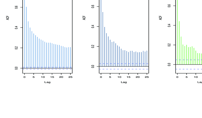
Figure 1: Auto covariance functions of $\mathbf{X}$ [left] and of two sub sampled processes corresponding to $\gamma=2.8$ [middle] and $\gamma=1.9$ [right]. The number of observed values of the sub sampled processes is equal to $5000$

In Figure 1 are depicted the empirical auto covariances of a trajectory of the process $X$ and of two sampled trajectories $Y_{1}$ and $Y_{2}$ . The memory parameter of $X$ is $d=0.35$ and the parameters of the two sampling distributions are respectively $\gamma_{1}=2.8$ and $\gamma_{2}=1.9$. According to Proposition 9, the process $Y_{1}$ has the same memory parameter as $X$, while the memory intensity is reduced for the process $Y_{2}$.

Then we estimate the memory parameters of the sampled processes by using the FEXP procedure introduced by [16, 2]. The FEXP estimator is adapted to processes having a spectral density. From Propositions 5 and 4, this is the case for our sampled processes. Figure 2 shows the estimate and a confidence interval. Two values, $d=0.1$ (lower curves) and $d=0.35$ (upper curves) of the memory parameter of $X$ are considered. In abscissa, the parameter $\gamma$ of the sampling distribution is allowed to vary between $1.7$ and $3.3$. From Proposition 9 the value of the memory parameter is $d$ if $\gamma\geq 2$ and $d-1+\gamma/2$ otherwise. In the case $d=0.1$ short memory is obtained for $\gamma<1.8$. In the case $d=0.35$, sample distributions leading to short memory are too heavy tailed to allow tractable simulations.

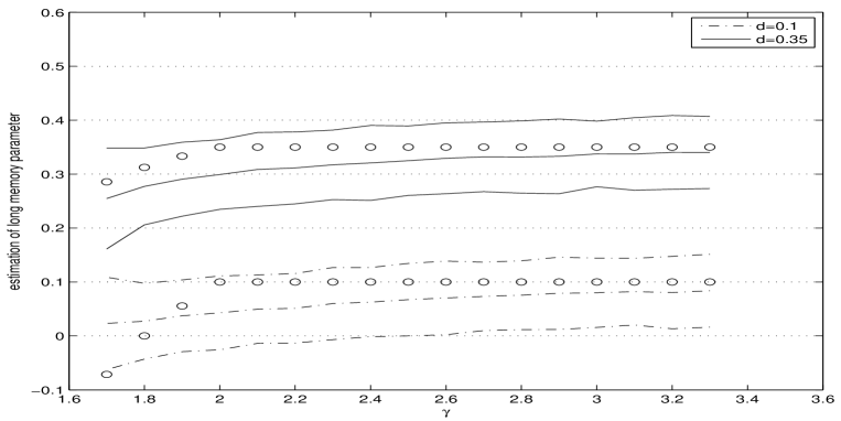
Figure 2: Estimation of the long memory parameter for $d=0.1$ and $d=0.35$ as function of parameter $\gamma$. The confidence regions are obtained using 500 independent replications. The circles represent the theoretical values of the parameter obtained in Proposition 9. For each $\gamma$, the estimation of $d$ is evaluated on $5000$ observations

4 Sampling generalised fractional processes

Consider now the family of generalised fractional processes whose spectral density has the form

$$f_{X}(\lambda)=|\Phi(\lambda)|^{2}\Big{|}\prod_{j=1}^{M}(e^{i\lambda}-e^{i\theta_{j}})^{-d_{j}}(e^{i\lambda}-e^{-i\theta_{j}})^{-d_{j}}\Big{|}^{2},$$ (4.33)

with exponents $d_{j}$ in $]0,1/2[$, and where $|\Phi(\lambda)|^{2}$ is the spectral density of an ARMA process.

4.1 Decrease of memory by heavy-tailed sampling law

See [11], [14], [19] for results and references on this class of processes. Taking $M=1$ and $\theta_{1}=0$, it is clear that this family includes the FARIMA processes, which belong to the framework of section 3. It is proved in [14] that as $h\to\infty$ the covariance sequence is a sum of periodic sequences damped by a regularly varying factor

$$\sigma_{X}(h)=h^{2d-1}\left(\sum c_{1,j}\cos(h\theta_{j})+c_{2,j}\sin(h\theta_{j})+o(1)\right)$$ (4.34)

where $d=\max\{d_{j};j=1,\ldots,M\}$ and where the sum extends over indexes corresponding to $d_{j}=d$. Hence, these models generally present seasonal long-memory, and for them the regular form $\sigma_{X}(h)=h^{2d-1}L(h)$ is lost. Precisely, this regularity remains only when, in (4.33), $d=\max\{d_{j};j=1,\ldots,M\}$ corresponds to the unique frequency $\theta=0$. In all other cases, from (4.34), it has to be to be replaced by

$$\sigma_{X}(h)=O(h^{2d-1}).$$

From the previous comments it is clear that Propositions 6 and 8 are no longer valid in the case of seasonal long-memory. That means that in this situation, it is not sure that long memory is preserved by a sampling law having a finite expectation. But it is true that long-memory can be lost. Indeed, Proposition 7 applies with $\alpha=1-2d$ where $d=\max\{d_{j};j=1,\ldots,M\}$, and the following result holds:

Proposition 10.

When sampling a process with spectral density (4.33) along a random walk such that the sampling law satisfies (3.29), the obtained process has short memory as soon as $1<\gamma<2(1-d)$ where $d=\max\{d_{j};j=1,\ldots,M\}$.

4.2 The effect of deterministic sampling

In a first step we just suppose that $\mathbf{X}$ has a spectral density $f_{X}$, which is unbounded in one or several frequencies (we call them singular frequencies). It is clearly the case of the generalised fractional processes. The examples shall be taken in this family. We investigate the effect of deterministic sampling on the number and the values of the singularities. Let us suppose that $S=\delta_{k}$, the law concentrated at $k$. It is well known that if $\mathbf{X}$ has a spectral density, the spectral density of the sampled process $\mathbf{Y}=(X_{kn})_{n}$ is

$$f_{Y}(\lambda) = \frac{1}{2\ell+1}\sum_{j=-l}^{l}f_{X}\left(\frac{\lambda-2\pi j}{2\ell+1}\right)\qquad\hbox{if}\;k=2\ell+1$$ (4.35)

$$f_{Y}(\lambda) = \frac{1}{2\ell}\left(\sum_{j=-\ell+1}^{\ell-1}f_{X}\left(\frac{\lambda-2\pi j}{2\ell}\right)+f_{X}\left(\frac{\lambda-2\pi\ell\hbox{sgn}(\lambda)}{2\ell}\right)\right)\qquad\hbox{if}\;k=2\ell$$

Proposition 11.

Let the spectral density of $(X_{n})_{n}$ have $N_{X}\geq 1$ singular frequencies. Then, denoting by $N_{Y}$ the number of singular frequencies of the spectral density of the sampled process $(Y_{n}=X_{kn})_{n}$

• $1\leq N_{Y}\leq N_{X}.$

• $N_{Y}<N_{X}$ if and only if $f_{X}$ has at least two singular frequencies $\lambda_{0}\neq\lambda_{1}$ such that, for some integer number $j^{*}$,

  $$\lambda_{0}-\lambda_{1}=\frac{2\pi j^{*}}{k}$$

Proof.

We choose $k=2\ell+1$ to simplify. The proofs for $k=2\ell$ are quite similar. Now remark that for fixed $j$,

$$\frac{\lambda-2\pi j}{2\ell+1}\in I_{j}:=\left[\frac{-\pi-2\pi j}{2\ell+1},\frac{\pi-2\pi j}{2\ell+1}\right[,\quad\hbox{for}\quad\lambda\in[-\pi,\pi[.$$

The intervals $I_{j}$ are non overlapping and $\cup_{j=-\ell}^{\ell}I_{j}=[-\pi,\pi[$. Now suppose that $f_{X}$ is unbounded at some $\lambda_{0}$. Then $f_{Y}$ is unbounded at the unique frequency $\lambda^{*}$ satisfying $\lambda_{0}=\frac{\lambda^{*}-2\pi j_{0}}{2\ell+1}$ for a suitable value $j_{0}$ of $j$. In other words, to every singular frequency of $f_{X}$ corresponds a unique singular frequency of $f_{Y}$. As a consequence, the number of singular frequencies of $f_{Y}$ is at least $1$, and cannot exceed the number of singularities of $f_{X}$.

It is clearly possible to reduce the number of singularities by deterministic sampling. Indeed, two distinct singular frequencies of $f_{X}$, $\lambda_{0}$ and $\lambda_{1}$ produce the same singular frequency $\lambda^{*}$ of $f_{Y}$ if and only if

$$\frac{\lambda^{*}-2\pi j_{0}}{2\ell+1}=\lambda_{0},\quad\hbox{and}\quad\frac{\lambda^{*}-2\pi j_{1}}{2\ell+1}=\lambda_{1},$$

which happens if and only if $\lambda_{0}-\lambda_{1}$ is a multiple of the basic frequency $\frac{2\pi}{2\ell+1}$.

∎

Proposition 11 is illustrated by the three following examples showing the various effects of the aliasing phenomenon when sampling generalised fractional processes.

We take $k=3$, so that the spectral density of $\mathbf{Y}$ is

$$f_{Y}(\lambda)=\frac{1}{3}\left(f_{X}\left(\frac{\lambda-2\pi}{3}\right)+f_{X}\left(\frac{\lambda}{3}\right)+f_{X}\left(\frac{\lambda+2\pi}{3}\right)\right).$$

Example 1.

Firstly consider $f_{X}(\lambda)=|e^{i\lambda}-1|^{-2d}$, the spectral density of the FARIMA ($0,d,0$) process. Then

$$f_{Y}(\lambda)=\frac{1}{3}\left(|e^{i\frac{\lambda-2\pi}{3}}-1|^{-2d}+|e^{i\frac{\lambda}{3}}-1|^{-2d}+|e^{i\frac{\lambda+2\pi}{3}}-1|^{-2d}\right)$$

has, on $[-\pi,\pi[$, only one singularity at $\lambda=0$, associated with the same memory parameter $d$ as for $f_{X}(\lambda)$. The memory of $\mathbf{Y}$ has the same characteristics as the memory of $\mathbf{X}$. This was already noticed in [7] and [12].

Example 2.

Consider now $f_{X}(\lambda)=|e^{i\lambda}-e^{\frac{2i\pi}{3}}|^{-2d}|e^{i\lambda}-e^{\frac{-2i\pi}{3}}|^{-2d}$, the spectral density of a long-memory seasonal process (see [19]). The sampled spectral density is

$$f_{Y}(\lambda)=\frac{1}{3}\sum_{j=-1}^{1}|e^{i\frac{\lambda-2\pi}{3}}-e^{\frac{2i\pi}{3}}|^{-2d}|e^{i\frac{\lambda-2\pi}{3}}-e^{\frac{-2i\pi}{3}}|^{-2d},$$

and is everywhere continuous on $[-\pi,\pi]$, except at $\lambda=0$ where

$$f_{Y}(\lambda)\sim c|\lambda|^{-2d}.$$

In other words the memory is preserved, but the seasonal effect disappears after sampling.

Example 3.

Consider now a case of two seasonalities ($\pm\pi/4$ and $\pm 3\pi/4$) associated with two different memory parameters $d_{1}$ and $d_{2}$:

$$f_{X}(\lambda)=|e^{i\lambda}-e^{\frac{i\pi}{4}}|^{-2d_{1}}|e^{i\lambda}-e^{\frac{-i\pi}{4}}|^{-2d_{1}}|e^{i\lambda}-e^{\frac{3i\pi}{4}}|^{-2d_{2}}|e^{i\lambda}-e^{\frac{-3i\pi}{4}}|^{-2d_{2}}.$$

It is easily checked that $f_{Y}$ has the same singular frequencies as $f_{X}$, with an exchange of the memory parameters:

$$f_{Y}(\lambda) \sim c\Big{|}\lambda\pm\frac{\pi}{4}\Big{|}^{-2d_{2}}\qquad\hbox{near}\;\mp\pi/4$$

$$f_{Y}(\lambda) \sim c\Big{|}\lambda\pm\frac{3\pi}{4}\Big{|}^{-2d_{1}}\qquad\hbox{near}\;\mp 3\pi/4.$$

5 Appendix

5.1 Proof of Lemma 2

Let us consider the two $z$-transforms of the bounded sequence $\sigma_{Y}(j)$:

$$\hat{\sigma}_{Y}^{-}(z) = \sum_{j=0}^{\infty}z^{j}\sigma_{Y}(j)\quad|z|<1$$

and

$$\hat{\sigma}_{Y}^{+}(z) = \sum_{j=0}^{\infty}z^{-j}\sigma_{Y}(j)\quad|z|>1.$$

On the first hand, from the representation

$$\sigma_{Y}(j)=\mathbb{E}(\sigma_{X}(T_{j}))=\int_{-\pi}^{\pi}f_{X}(\lambda)\hat{S}(\lambda)^{j}d_{\lambda},$$

we have

$$\hat{\sigma}_{Y}^{-}(z) = \sum_{j=0}^{\infty}z^{j}\int_{-\pi}^{\pi}f(\lambda)\left(\hat{S}(\lambda)\right)^{j}d\lambda=\int_{-\pi}^{\pi}\frac{f(\lambda)}{1-z\hat{S}(\lambda)}d\lambda,\quad|z|<1\;$$ (5.36)

$$\hat{\sigma}_{Y}^{+}(z) = \sum_{j=0}^{\infty}z^{-j}\int_{-\pi}^{\pi}f(\lambda)\left(S(\lambda)\right)^{j}d\lambda=\int_{-\pi}^{\pi}\frac{f(\lambda)}{1-\frac{\hat{S}(\lambda)}{z}}d\lambda,\quad|z|>1\;$$ (5.37)

On the second hand, let $C_{r}$ be the circle $|z|=r$. If $0<r<1$, for all $j\geq 0$

$${\frac{1}{2i\pi}}\int_{C_{r}}\hat{\sigma}_{Y}^{-}(z)z^{-j-1}dz = {\frac{1}{2\pi}}\int_{-\pi}^{\pi}(re^{i\theta})^{-j}\hat{\sigma}_{Y}^{-}(re^{i\theta})d\theta$$ (5.38)

$$= \sum_{l=0}^{\infty}{\frac{r^{l-j}\sigma_{Y}(l)}{2\pi}}\int_{-\pi}^{\pi}e^{i(l-j)\theta}d\theta=\sigma_{Y}(j),$$

and, similarly, if $r>1$

$${\frac{1}{2i\pi}}\int_{C_{r}}\hat{\sigma}_{Y}^{+}(z)z^{j-1}dz = {\frac{1}{2\pi}}\int_{-\pi}^{\pi}(re^{i\theta})^{j}\hat{\sigma}_{Y}^{+}(re^{i\theta})d\theta$$ (5.39)

$$= \sum_{l=0}^{\infty}{\frac{r^{j-l}\sigma_{Y}(l)}{2\pi}}\int_{-\pi}^{\pi}e^{i(j-l)\theta}d\theta=\sigma_{Y}(j),$$

Gathering (5.36) with (5.38) and (5.37) with (5.39) leads to

$$\sigma_{Y}(j)=\begin{cases}{\frac{1}{2\pi}}\int_{-\pi}^{\pi}e^{-ij\theta}\left(r^{-j}\int_{-\pi}^{\pi}\frac{f(\lambda)}{1-re^{i\theta}\hat{S}(\lambda)}d\lambda\right)d\theta,&\text{if $r<1$}\\ {\frac{1}{2\pi}}\int_{-\pi}^{\pi}e^{ij\theta}\left(r^{j}\int_{-\pi}^{\pi}\frac{f(\lambda)}{1-\frac{e^{-i\theta}\hat{S}(\lambda)}{r}}d\lambda\right)d\theta,&\text{if $r>1$}\\ \end{cases}$$ (5.40)

Changing the integrand in (5.40) into its conjugate when $r<1$, and $r$ for $1/r$ when $r>1$ leads to gives

$$\sigma_{Y}(j)=r^{-j}\int_{-\pi}^{\pi}e^{ij\theta}g(r,\theta)d\theta,,\qquad\forall r\in[0,1[$$ (5.41)

where $g(r,\theta)$ is defined in (2.6). As the first member does not depend on $r$, (2.5) is proved.

Let us now prove (2.7). Firstly,

$$Im\left(\frac{1}{1-re^{-i\theta}\hat{S}(\lambda)}+\frac{1}{1-re^{-i\theta}\hat{S}(-\lambda)}\right)\\ =\frac{1}{2}\left(\frac{1}{1-re^{-i\theta}\hat{S}(\lambda)}+\frac{1}{1-re^{-i\theta}\hat{S}(-\lambda)}-\frac{1}{1-re^{i\theta}\hat{S}(-\lambda)}-\frac{1}{1-re^{i\theta}\hat{S}(\lambda)}\right)$$

is an odd function of $\lambda$. Hence, the imaginary part of the integrand in (2.6) disappears after integration.

Secondly,

$$Re\left(\frac{1}{1-re^{-i\theta}\hat{S}(\lambda)}+\frac{1}{1-re^{-i\theta}\hat{S}(-\lambda)}\right)\\ =\frac{1}{2}\left(\frac{1-r^{2}|\hat{S}(\lambda)|^{2}}{|1-re^{-i\theta}\hat{S}(\lambda)|^{2}}+\frac{1-r^{2}|\hat{S}(\lambda)|^{2}}{|1-re^{-i\theta}\hat{S}(-\lambda)|^{2}}+2\right),$$ (5.42)

and the proof is over.

5.2 A few technical results

Hereafter we recall some properties used in the paper.

Lemma 12.

The Poisson kernel (2.4) satisfies

$$2\pi P_{s}(t)\leq\frac{1-s^{2}}{(1-s)^{2}}=\frac{1+s}{1-s}\leq\frac{2}{\eta}\qquad\forall s<1-\eta,\quad\hbox{with}\;s<1.$$ (5.43)

$$0<\delta<|t|\leq\frac{\pi}{2}\Longrightarrow P_{s}(t)<P_{s}(\delta).$$ (5.44)

$$2\pi\sup_{0<s<1}P_{s}(t)=\frac{1}{|\sin t|}\qquad\forall t\in]-\pi/2,\pi/2[.$$ (5.45)

Proof.

The bound (5.43) is direct. Inequality (5.44) comes from the monotonicity of the kernel with respect to $s$.

Let us prove (5.45):

$$\frac{\partial}{\partial s}\left(P_{s}(t)\right)=2\frac{s^{2}\cos t-2s+\cos t}{(1+s^{2}-2s\cos t)^{2}}.$$

It is easily checked that the numerator has one single root $s_{0}=\frac{1-|\sin t|}{\cos t}$ in $[0,1[$, and $P_{s_{0}}(t)=|\sin t|^{-1}.$ ∎

The following result comes from spectral considerations.

Lemma 13.

With $\rho=\rho(\lambda)$ and $\tau=\tau(\lambda)$ defined in (2.9), for all $r\in[0,1[$ and $\theta\in]-\pi,\pi[$,

$$g^{*}(r,\theta):=\frac{1}{4}\int_{-\pi}^{\pi}\left(\frac{1}{\pi}+P_{r\rho}(\tau-\theta)+P_{r\rho}(\tau+\theta)\right)d\lambda=1$$ (5.46)

Proof.

Notice first that if $f_{X}\equiv 1$, the process $X$ is a white noise with $\mathrm{Var}(X_{1})=2\pi$. Hence, the sampled process is also a white noise with variance $2\pi$. Applying (2.6) to a white noise, we get

$$2\pi\delta_{0}(j)=r^{-j}\int_{-\pi}^{\pi}e^{ij\theta}g^{*}(r,\theta)d\theta.$$ (5.47)

for all $r\in[0,1[$. Since $r^{j}\delta_{0}(j)=\delta_{0}(j)$, we can rewrite (5.47) as

$$2\pi\delta_{0}(j)=\int_{-\pi}^{\pi}e^{ij\theta}g^{*}(r,\theta)d\theta.$$

This means that $g^{*}(r,\theta)$ is the Fourier transform of $(2\pi\delta_{0}(j))_{j}$. Consequently $g^{*}(r,\theta)\equiv 1$. ∎

5.3 Proof of Proposition 4

As for Proposition 3, the proof consists in finding an integrable function $g(\theta)$ such that

$$|g(r,\theta)|\leq g(\theta)\quad\forall r\in]0,1[,\theta\in]-\pi,\pi[.$$ (5.48)

For that purpose, we need the following estimation of $\hat{S}(\lambda)$ near zero.

$$|1-\hat{S}(\lambda)| = \Big{|}(1-e^{i\lambda})\sum_{j\geq 1}S(j)\frac{1-e^{ij\lambda}}{1-e^{i\lambda}}\Big{|}=|1-e^{i\lambda}|\Big{|}\sum_{j\geq 1}S(j)e^{\frac{(j-1)\lambda}{2}}\frac{\sin(j\lambda/2)}{\sin\lambda/2}\Big{|}$$ (5.49)

$$\leq |1-e^{i\lambda}|\sum_{j\geq 1}jS(j)$$

$$= |2i\sin(\lambda/2)e^{i\lambda/2}|\sum_{j\geq 1}jS(j)=2|\sin(\lambda/2)|\sum_{j\geq 1}jS(j)\leq|\lambda|\sum_{j\geq 1}jS(j)$$

$$= C|\lambda|.$$

Now we use the fact that

$$|u|\leq u_{0}<1\Longrightarrow|1-u|>1-u_{0}\quad\hbox{and}\quad\sin(\arg(1-u))<u_{0}.$$

Since $u_{0}<\pi/2$, this implies $\arg(1-u)<\pi u_{0}/2$.

From this and inequality (5.49) we obtain

$$|\lambda|\leq\frac{1}{C}\Longrightarrow|\tau(\lambda)|\leq\frac{\pi C|\lambda|}{2}$$ (5.50)

For a fixed $\theta>0$ let $\lambda_{0}$ be such that $\phi$ is bounded on $[-\lambda_{0},\lambda_{0}]$. Denoting

$$b(\theta)=\min\left\{\lambda_{0},\frac{1}{C},\frac{\theta}{\pi C}\right\},$$

we separate $[-\pi,\pi]$ into four intervals:

$$[-\pi,-b(\theta)[,\;[-b(\theta),0[,\;]0,b(\theta)],\;]b(\theta),\pi].$$

In the sequel we only deal with the two last intervals, and concerning the integrand in (2.7) we only treat the part $P_{r\rho}(\tau-\theta)$:

$$I_{1}(\theta)+I_{2}(\theta) = \int_{0}^{b(\theta)}f(\lambda)P_{r\rho(\lambda)}(\tau(\lambda)-\theta)d\lambda+$$

$$+ \int_{b(\theta)}^{\pi}f(\lambda)P_{r\rho(\lambda)}(\tau(\lambda)-\theta)d\lambda.$$

$\bullet$ Bounding $I_{1}$:

From (5.50), since $b(\theta)\leq\theta/(\pi C)$, we have $|\tau(\lambda)|\leq\theta/2$ which implies

$$\frac{\theta}{2}\leq|\tau(\lambda)-\theta|.$$

Via (5.44) and (5.45), this leads to

$$P_{r\rho}(\tau-\theta)\leq P_{r\rho}(\theta/2)\leq\frac{1}{2\theta}.$$

Consequently

$$I_{1} \leq \frac{\sup_{[0,b(\theta)]}(\phi(\lambda))}{2\theta}\int_{0}^{b(\theta)}\lambda^{-2d}d\lambda=\frac{\sup_{[0,b(\theta)]}(\phi(\lambda))}{2\theta}(b(\theta))^{-2d+1}$$

$$\leq C_{1}\theta^{-2d}$$

since $b(\theta)\leq\theta/(\pi C)$ and $-2d+1>0$.

$\bullet$ Bounding $I_{2}$:

When $\lambda>b(\theta)$, we have $\lambda^{-2d}\leq C_{2}\max\{\theta^{-2d},1\}$ for some constant $C_{2}$. Hence

$$I_{2}\leq C_{2}\max\{\theta^{-2d},1\}\int_{-\pi}^{\pi}\phi(\lambda)P_{r\rho}(\theta-\tau)d\lambda.$$ (5.51)

Since $\phi$ is bounded in a neighbourhood of zero, the arguments used to prove Proposition 3 show that the integral in (5.51) is bounded by a constant.

Finally $I_{1}+I_{2}$ is bounded by an integrable function $g(\theta)$ and the proposition is proved.

5.4 Proof of Proposition 5

The following lemma gives the local behaviour of $\hat{S}(\lambda)$ under assumption (2.13).

Lemma 14.

Since $S(j)\sim cj^{-\gamma}$ with $1<\gamma<2$ and $c>0$,

$$|\lambda|^{1-\gamma}(1-\hat{S}(\lambda))\to Z,\;\hbox{if}\;\lambda\to 0.$$ (5.52)

where $Re(Z)>0$ and $Im(Z)<0$.

Proof.

From the assumption on $S(j)$,

$$\sum_{j\geq 1}S(j)(1-\cos(j\lambda)) \sim_{\lambda\to 0} c\sum_{j\geq 1}j^{-\gamma}(1-\cos(j\lambda))$$

and

$$\sum_{j\geq 1}S(j)\sin(j\lambda) \sim_{\lambda\to 0} c\sum_{j\geq 1}j^{-\gamma}\sin(j\lambda).$$

Then, using well known results of Zygmund ([23]; pages 186 and 189)

$$\sum_{j\geq 1}j^{-\gamma}(1-\cos(j\lambda)) \sim_{\lambda\to 0} \frac{c}{\gamma-1}|\lambda|^{\gamma-1}=:c_{1}|\lambda|^{\gamma-1}.$$

and

$$\sum_{j\geq 1}j^{-\gamma}\sin(j\lambda) \sim_{\lambda\to 0} c\Gamma(1-\gamma)\cos\left(\frac{\pi\gamma}{2}\right)|\lambda|^{\gamma-1}=:c_{2}|\lambda|^{\gamma-1}$$

It is clear that $c_{1}>0$, and $c_{2}<0$ follows from the fact that $\Gamma(x)<0$ for $x\in]-1,0[$ and $\cos\left(\pi\gamma/2\right)<0$. ∎

In the sequel we take $\lambda>0$. From this lemma, if $\lambda$ is small enough (say $0\leq\lambda\leq\lambda_{0}$),

$$c_{3}\lambda^{\gamma-1}\leq \tau(\lambda) \leq c^{\prime}_{3}\lambda^{\gamma-1}$$ (5.53)

and

$$1-c_{4}\lambda^{\gamma-1}\leq \rho(\lambda) \leq 1-c^{\prime}_{4}\lambda^{\gamma-1}$$ (5.54)

where the constants are positive.

For a fixed $\theta>0$, we deduce from (5.53)

$$\lambda<\min\left\{\lambda_{0},\left(\frac{\theta}{c^{\prime}_{3}}\right)^{1/(\gamma-1)}\right\}\quad\hbox{implies}\quad 0<\theta-c^{\prime}_{3}\lambda^{\gamma-1}\leq\theta-\tau(\lambda)$$ (5.55)

After choosing $\lambda_{1}\leq\lambda_{0}$ such that $\phi$ is bounded on $[0,\lambda_{1}]$ define

$$c(\theta)=\min\left\{\lambda_{1},\left(\frac{\theta}{c^{\prime}_{3}}\right)^{1/(\gamma-1)}\right\}.$$

Then we split $[-\pi,\pi]$ into six intervals

$$[-\pi,-\lambda_{1}[,\;[-\lambda_{1},-c(\theta)/2[,\;[-c(\theta)/2,0[,\;]0,c(\theta)/2],\;]c(\theta)/2,\lambda_{1}],\;]\lambda_{1},\pi].$$

We only consider the integral on the three last domains and the part $P_{r\rho}(\tau-\theta)$ of the integrand in (2.7).

$\bullet$ When $\lambda\in]0,c(\theta)/2]$, inequality (5.55) and properties (5.44) and (5.45) of the Poisson kernel lead to

$$P_{r\rho}(\theta-\tau)\leq P_{r\rho}(\theta-c^{\prime}_{3}\lambda^{\gamma-1})\leq\frac{C}{\theta-c^{\prime}_{3}\lambda^{\gamma-1}},$$

whence

$$I_{1} = \int_{0}^{c(\theta)/2}f(\lambda)P_{r\rho}(\theta-\tau)d\lambda\leq C^{\prime}_{1}\int_{0}^{c(\theta)/2}\frac{\lambda^{-2d}}{\theta-c^{\prime}_{3}\lambda^{\gamma-1}}d\lambda$$

$$\leq C^{\prime}_{1}\int_{0}^{\frac{1}{2}\left(\frac{\theta}{c^{\prime}3}\right)^{1/(\gamma-1)}}\frac{\lambda^{-2d}}{\theta-c^{\prime}_{3}\lambda^{\gamma-1}}d\lambda$$

$$= C^{\prime}_{2}\theta^{\frac{-2d+1}{\gamma-1}-1}\int_{0}^{2^{-\frac{1}{\gamma-1}}}\frac{u^{\frac{-2d+1}{\gamma-1}-1}}{1-u}du.$$

Since $\frac{-2d+1}{\gamma-1}-1>-1$, the last integral is finite, implying

$$I_{1}\leq C^{\prime}_{3}\theta^{\frac{-2d+1}{\gamma-1}-1},$$

which is an integrable function of $\theta$.

$\bullet$ Thanks to (5.43) and to the r.h.s. of (5.54), we have on the interval $]c(\theta)/2,\lambda_{1}]$

$$P_{r\rho}(\theta-\tau)\leq\frac{C^{\prime}_{3}}{\lambda^{\gamma-1}}.$$

Since $\phi$ is bounded on this domain,

$$I_{2} \leq C^{\prime}_{3}\sup_{0<\lambda\leq\lambda_{1}}{\phi(\lambda)}\int_{c(\theta)/2}^{\lambda_{1}}\lambda^{-2d+1-\gamma}d\lambda$$

$$= \frac{C^{\prime}_{3}\sup_{0<\lambda\leq\lambda_{1}}{\phi(\lambda)}}{-2d+2-\gamma}\left(\lambda_{1}^{-2d+2-\gamma}-(c(\theta)/2)^{-2d+2-\gamma}\right)$$

$$\leq \frac{C^{\prime}_{3}\sup_{0<\lambda\leq\lambda_{1}}{\phi(\lambda)}}{-2d+2-\gamma}\left(\lambda_{1}^{-2d+2-\gamma}+(c(\theta)/2)^{-2d+2-\gamma}\right)$$

$$= C^{\prime}_{4}\left(\lambda_{1}^{-2d+2-\gamma}+\left(\min\left\{\lambda_{1},\left(\frac{\theta}{c^{\prime}3}\right)^{1/(\gamma-1)}\right\}\right)^{-2d+2-\gamma}\right).$$

where the function between brackets is integrable because

$$\frac{-2d+2-\gamma}{\gamma-1}=\frac{-2d+1}{\gamma-1}-1>-1.$$

$\bullet$ Finally,

$$I_{3}=\int_{\lambda_{1}}^{\pi}f(\lambda)P_{r\rho}(\theta-\lambda)d\lambda\leq\lambda_{1}^{-2d}\int_{-\pi}^{\pi}\phi(\lambda)P_{r\rho}(\theta-\lambda)d\lambda$$

which has already been treated since $\phi$ is bounded near zero.

Gathering the above results on $I_{1}$, $I_{2}$ and $I_{3}$ completes the proof.

References

• [1] Bardet, JM; Lang, G.; Oppenheim, G; Philippe, and Taqqu, M (2002) Generators of long-range dependent processes : A survey. In Long-Range Dependence : Theory and Applications. Eds Doukhan, Taqqu and Oppenheim birkhauser Boston.
• [2] Bardet, J.M.; Lang, G. ; Oppenheim, G.; Philippe, A. Stoev, S. and Taqqu, M. (2003). Semi-parametric estimation of the long-range dependent processes : A survey. In Long-Range Dependence : Theory and Applications. Eds Doukhan, Taqqu and Oppenheim birkhauser Boston
• [3] Beutler R. J. (1970) Alias-free Randomly Timed Sampling of Stochastic Processes. IEEE Trans. Inf. Theory. Vol. IT-16 (2). pp 147–152.
• [4] Bingham N. H., Goldie C. M. and Teugels J. L. (1987) Regular variation. Encyclopedia of Mathematics. Cambridge U. Press.
• [5] Brewer K. (1975) Some consequences of temporal aggregation and systematic sampling for ARMA or ARMAX models. J. Econom. 1, 133–154.
• [6] Brockwell P. J. , Davis R. A. (1991) Time Series: Theory and Methods. Springer Verlag. New York.
• [7] Chambers M., (1998). Long-memory and aggregation in macroeconomic time-series. International Economic Rev. 39, 1053–1072.
• [8] Ding Z., Granger C. W. J. , Engle R. F. (1992) A long Memory Property of Stock Market Returns and a New Model. Discussion paper 92-21, Department of Economics, University of California, San Diego.
• [9] Feller W. (1971)An Introduction to Probability Theory and Applications Vol. II. Wiley.
• [10] Granger C. W. J., Joyeux R. (1980) An introduction to long memory time series models and fractional differencing. J. Time Ser. Anal. 1, 15–29.
• [11] Gray H. L., Zhang N. F., Woodward W. A. (1989). On generalized fractional processes. J. Time Ser. Anal. 10, 233–257.
• [12] Hwang S. (2000). The Effects of Systematic Sampling and Temporal Aggregation on Discrete Time Long Memory Processes and Their Finite Sample Properties. Econometric Theory. 16, 347-372
• [13] Kadi A., Oppenheim G., Viano M.-C. (1994). Random aggregation of uni and multivariate linear processes, J. Time Ser. Anal. 15, 31–44.
• [14] Leipus R., Viano M.-C. (2000). Modelling long-memory time series with finite or infinite variance: a general approach. J. Time Ser. Anal. 21, 61–74.
• [15] Masry E.(1971). Random Sampling and Reconstruction of Spectra. Information and Control Vol. 19 (4): 275-288.
• [16] Moulines E. Soulier Ph. (1999) Log-periodogram regression of time series with long range dependence Annals of statistics, 27(4), 1415-1439.
• [17] Niemi H. (1984) The invertibility of sampled and aggregate ARMA models. Metrika 31, 43–50.
• [18] Oppenheim G. (1982) Échantillonnage aléatoire d’un processus ARMA. C. R. Acad. Sci. Paris Sér. I Math. 295 (1982), no. 5, 403–406.
• [19] Oppenheim G., Ould Haye M., Viano M.-C. (2000) long-memory with seasonal effects. Stat. Inf. for Stoch. Proc. Vol. 3, 53–68.
• [20] Shapiro H. S., Silverman R. A. (1960). Alias-Free Sampling of Random Noise. Journal of the Society for Industrial and Applied Mathematics, Vol. 8-2, 225-248
• [21] Sram D. O., Wei W. S. (1986). Temporal aggregation in the ARIMA processes. J. Time Ser. Anal. 7, 279–292.
• [22] Stout W. F. (1974). Almost sure convergence. Academic Press New York.
• [23] Zygmund A. (1959) Trigonometric series. Vol 1. Camb. Un. Press.