Momentum-space interferometry with trapped ultracold atoms

Abstract

Quantum interferometers are generally set so that phase differences between paths in coordinate space combine constructive or destructively. Indeed, the interfering paths can also meet in momentum space leading to momentum-space fringes. We propose and analyze a method to produce interference in momentum space by phase-imprinting part of a trapped atomic cloud with a detuned laser. For one-particle wave functions analytical expressions are found for the fringe width and shift versus the phase imprinted. The effects of unsharpness or displacement of the phase jump are also studied, as well as many-body effects to determine the potential applicability of momentum-space interferometry.

I Introduction

In most quantum interferometers the phase differential between paths that meet in a coordinate-space point or region at a given time lead to constructive or destructive wave combinations and thus to fringes, but the paths can also interfere in momentum space and produce momentum-space fringes. In particular, during the crossing of a wavepacket over a small and thin barrier (compared to the energy and width of the wavepacket), see Fig. 1a, the momentum distribution can change dramatically, vanishing at the center of the distribution, and being enhanced at the wings. This process would violate classical energy-conservation PRL98 , and is due to interference in momentum space between incident and transmitted parts of the wave PRA01 ; PRA05 .

The experimental implementation of this effect is in principle possible with current cold-atom technology, by turning off an effective detuned-laser barrier in the midst of the wavepacket passage, but a version which is simpler to implement is described here. The effect of the scattering barrier in the original proposal is to imprint an appropriate phase on approximately half of the wavepacket, and this can also be achieved by shining part of a trapped, initially stationary, wavepacket with a strong laser pulse, during a short time in the scale in which a perturbation propagates (the correlation time BS04 ), see Fig. 1b. The phase imprinting technique was first introduced with the purpose of generating vortices Lewenstein99 ; Cornell01 . Here we shall study the properties of the resulting fringes, and show that the effect on the momentum distribution is similar to the effect of the scattering process, with the creation of a vanishing point (“dark notch”) at the center and enhancement of the wings. Furthermore, we shall study the shift, width and visibility of this central “dark notch” as a function of the imprinted phase, as a necessary step to determine the potential applicability of momentum-space interferometry. The imprinted phase carries information about the laser interaction (time, laser intensity, frequency) that can be obtained from the notch. By immediately removing the external trap, the momentum distribution is essentially frozen after the imprinting, and many-body effects cease to play a role. Then, the momentum-space notch will become by expansion a coordinate-space notch measurable with standard time-of-flight techniques. Alternatively, the momentum distribution can be accessed by stimulated Raman transitions GW01 or through the single-particle reduced density matrix Bloch .

In the following section we will describe the setting in more detail for a single particle or many non-interacting particles. In Section III we will consider the role of interactions within the mean-field regime and in Section IV we will look at Tonks-Girardeau and non-interacting Fermi gases.

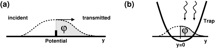
Figure 1: Schematic settings: (a) phase imprinting caused by wave packet passage above a weak, narrow potential, (b) phase imprinting caused by illumination with a detuned laser of a trapped wave packet.

II Non-Interacting Regime

We start considering the non-interacting regime in which the single-particle description is valid. A highly anisotropic three-dimensional harmonic trap is assumed, so that the transverse degrees of freedom remain frozen and the system becomes effectively one-dimensional, along the axis with lowest trap frequency $\omega$. It is useful to introduce dimensionless variables, namely a dimensionless position $y=\sqrt{\frac{m\omega}{\hbar}}x$, where $x$ is the dimensional position and $m$ the mass of the single particle, and a dimensionless momentum $q=\sqrt{\frac{\hbar}{m\omega}}k$, where $k$ is the dimensional wavenumber. The Hamiltonian describing the system is $H=-\frac{\hbar^{2}}{2m}\frac{\partial^{2}}{\partial x^{2}}+\frac{m\omega^{2}}{2}x^{2}$ and in the above dimensionless variables we get $H=\frac{\hbar\omega}{2}\left(-\frac{\partial^{2}}{\partial y^{2}}+y^{2}\right)$. The corresponding eigenvalues are $E_{n}=\frac{\hbar\omega}{2}(2n+1)$ and the eigenstates are $\psi_{n}(y)=\frac{1}{\sqrt{2^{n}n!\sqrt{\pi}}}H_{n}(y)e^{-y^{2}/2}$, where $H_{n}(y)$ is the $n$-th Hermite polynomial. The eigenstates are normalized such that $\int dy\,\psi_{n}(y)\psi_{m}(y)=\delta_{n,m}$.

Initially, the trapped particle is described by the wavefunction $\psi_{0}(y)$ in coordinate space. Then a phase is imprinted on the right hand side of the trap, i.e. for $y>0$. For atoms, this can be achieved by shining an appropriate detuned laser pulse for a short time $t$. The detuned laser acts as a mechanical potential $V\Theta(y)$ on the atom, where $V=\Omega^{2}\hbar/4\Delta$, $\Omega$ is the Rabi frequency, and $\Delta$ the detuning (laser frequency minus transition frequency). If the time $t$ is short, the effect is to imprint a phase $\varphi=-Vt/\hbar$ on the wave function for $y>0$. The wavefunction in coordinate space becomes $\psi_{0}(y)e^{i\varphi w(y)}$ with $w(y)=\Theta(y)$, and in momentum space

$$\phi_{0}(q) = \frac{1}{\sqrt{2\pi}}\int_{-\infty}^{0}dy\,\psi_{0}(y)e^{-iqy}$$

$$+ e^{i\varphi}\frac{1}{\sqrt{2\pi}}\int_{0}^{\infty}dy\,\psi_{0}(y)e^{-iqy}.$$

Each momentum gets an amplitude contribution from two different terms and we may expect interferences in $\left|\phi_{0}(q)\right|^{2}$ for $\varphi>0$. In the following, this interference pattern will be studied and analytical expressions will be found for the fringe shift, width and visibility versus the phase $\varphi$ imprinted. The effects of unsharpness or spatial displacement of the phase jump are also studied.

II.1 Reference Case

Let us first study the effect of imprinting a phase $\varphi$ on the ground state of the harmonic trap, $n=0$. In this case the momentum probability density becomes

$$\left|\phi_{0}(q)\right|^{2}=\frac{e^{-q^{2}}}{\sqrt{\pi}}\left|\cos\left(\frac{\varphi}{2}\right)+\sin\left(\frac{\varphi}{2}\right)\mbox{erfi}\left(\frac{q}{\sqrt{2}}\right)\right|^{2},$$ (1)

which has a zero at $q_{0}$, a solution of

$$\mbox{erfi}\left(\frac{q_{0}}{\sqrt{2}}\right)=-\mbox{cot}\left(\frac{\varphi}{2}\right).$$ (2)

Momentum distributions for this reference case after different phase imprintings are displayed in Fig. 2a. Note the optimality of $\varphi=\pi$ to produce a deep minimum, in fact a zero, exactly at the peak of the original distribution, $q_{0}=0$, and the enhancement at the wings. In the following, we will concentrate on this central “dark notch”. The “motion” of $q_{0}$ with $\varphi$ can be seen in Fig. 2a, and in more detail in Fig. 3a (solid line), where $q_{0}$ is plotted versus $\varphi$. It shows a linear behavior in $\pi/2<\varphi<3\pi/2$ and slight deviations beyond that range. The width $\Delta q=q_{+}-q_{-}$ of the central interference dip is defined as the difference between the momentum $q_{+}$ of the maximum on the right-hand side of the minimum and the momentum $q_{-}$ of the maximum on the left-hand side. Fig. 3b (solid line) shows the width versus the phase. Note that the width is always greater that $\sqrt{2\pi}$ (value of the thick dotted line).

Another important quantity is the visibility of the minimum, which we define as

$$v=\frac{\min_{\pm}\left(\left|\phi_{0}(q_{\pm})\right|^{2}-\left|\phi_{0}(q_{0})\right|^{2}\right)}{\frac{\left|\phi_{0}(q_{+})\right|^{2}+\left|\phi_{0}(q_{-})\right|^{2}}{2}+\left|\phi_{0}(q_{0})\right|^{2}}.$$

This visibility is plotted in Fig. 3c (solid line). From the calculations we can infer that the visibility limits the working range of the interferometer to $\pi/2<\phi<3\pi/2$, and is optimal around $\phi=\pi$.

Figure 2: Wave function in momentum space for different phase imprintings $\varphi$; (a) reference case, $y_{0}=0$, $\zeta=0$, (b) effect of shifting, $y_{0}=0.3$, $\zeta=0$, (c) effect of smoothing, $y_{0}=0$, $\zeta=0.1$, (d) effect of interaction, solution of the GPE: $y_{0}=0$, $\zeta=0$, $g=20$.

Figure 3: (a) Momentum of the minimum versus $\varphi$, (b) width of the minimum versus $\varphi$, (c) visibility of the minimum versus $\varphi$; in all cases $n=0$.
Analytical approximations: thick dotted lines: $\tilde{v}$, $\widetilde{\Delta q}$, $\tilde{q}_{0}$; dotted lines: $\bar{v}$, $\overline{\Delta q}$, $\bar{q}_{0}$ (Thomas-Fermi with $g=20$).
Exact results: solid line: reference case, $v$, $\Delta q$, $q_{0}$ with $y_{0}=0,\zeta=0$; boxes: effect of shifting, $v$, $\Delta q$, $q_{0}$ with $y_{0}=0.3,\zeta=0$; triangles: effect of smoothing, $v$, $\Delta q$, $q_{0}$ with $y_{0}=0,\zeta=0.1$; circles: effect of interaction, $v$, $\Delta q$, $q_{0}$ based on the solution of the GPE with $y_{0}=0,\zeta=0,g=20$.

II.2 Analytical approximations for the reference case

The goal now is to derive approximate analytical formulae describing the properties of the central “dark notch” as a function of the imprinted phase. From $\frac{\partial\left|\phi_{0}(q)\right|^{2}}{\partial q}=0$, we get the extreme points of $\left|\phi_{0}(q)\right|^{2}$ as solutions of

$$\overbrace{\left(\cos\left(\frac{\varphi}{2}\right)+\sin\left(\frac{\varphi}{2}\right)\mbox{erfi}\left(\frac{q}{\sqrt{2}}\right)\right)}^{z_{1}}$$ (3)

$$\times \underbrace{\left(q\cos\left(\frac{\varphi}{2}\right)-\sin\left(\frac{\varphi}{2}\right)\left(e^{q^{2}/2}\sqrt{\frac{2}{\pi}}-q\,\mbox{erfi}\left(\frac{q}{\sqrt{2}}\right)\right)\right)}_{z_{2}}$$

$$= 0.$$

Note that if $q$ is a solution of (3) for $\varphi=\pi+\Delta\varphi$ then $-q$ is a solution for $\varphi=\pi-\Delta\varphi$.

One of the solutions of equation (3) fulfilling $z_{1}=0$ and describing the momentum of the minimum is approximately given by

$$q_{0}\approx\sqrt{\frac{\pi}{2}}\frac{\varphi-\pi}{2}=:\tilde{q}_{0}$$ (4)

(based on a linearization of $z_{1}=0$ around $\varphi\approx\pi$ and $q\approx 0$). This describes a linear displacement of the minimum with $\varphi$. Fig. 3a shows the exact momentum of the minimum $q_{0}$ (solid line) and $\tilde{q}_{0}$ (thick dotted line) versus $\varphi$.

Now we shall obtain expressions for the (momentum of the) left maximum, $q_{-}$, and the right maximum $q_{+}$. An approximate solution of $z_{2}=0$ is

$$q_{+}\approx\frac{\varphi}{\sqrt{2\pi}}=:\tilde{q}_{+},$$

which follows from a linearization of $z_{2}=0$ around $\varphi\approx 0$ and $q\approx 0$. Another approximate solution of $z_{2}=0$ is

$$q_{-}\approx-\frac{2\pi-\varphi}{\sqrt{2\pi}}=:\tilde{q}_{-},$$

obtained by linearizing $z_{2}=0$ around $\varphi\approx 2\pi$ and $q\approx 0$. Thus we get for the the width of the interference dip

$$\Delta q=q_{+}-q_{-}\approx\tilde{q}_{+}-\tilde{q}_{-}=\sqrt{2\pi}=:\widetilde{\Delta q}.$$

Figure 3b compares the numerically calculated exact width $\Delta q$ (solid line) with $\widetilde{\Delta q}$ (thick dotted line).

We can also find a simple expression for the visibility. From Eq. (1) and using also the approximations of the momentum of the two maxima and the minima and retaining only the first order in $\varphi$ we get

$$\left|\phi_{0}(q_{-})\right|^{2} \approx \alpha+\beta(\varphi-\pi),$$

$$\left|\phi_{0}(q_{0})\right|^{2} \approx 0,$$

$$\left|\phi_{0}(q_{+})\right|^{2} \approx \alpha-\beta(\varphi-\pi),$$

where

$$\alpha = \frac{e^{-\pi/2}}{\sqrt{\pi}}\mbox{erfi}\left(\frac{\sqrt{\pi}}{2}\right)^{2}\approx 0.210,$$

$$\beta = \frac{e^{-\pi/2}}{\pi^{3/2}}\mbox{erfi}\left(\frac{\sqrt{\pi}}{2}\right)\left(-2e^{\pi/4}+\pi+\pi\mbox{erfi}\left(\frac{\sqrt{\pi}}{2}\right)\right)$$

$$\approx 0.148.$$

The final result is

$$v\approx 1-\frac{\beta}{\alpha}\left|\varphi-\pi\right|=:\tilde{v},$$

also shown in Fig. 3c (thick dotted line). It gives a lower bound for the exact result $v$ (solid line).

II.3 Perturbations of the reference case

In this subsection we examine the effect of perturbations of the reference case. First we want to discuss the effect of shifting the edge of the phase imprinted region, $y_{0}$, out of the center of the trap, i.e. we have $w(z)=\Theta(y-y_{0})$. Right after the phase-imprinting, the $0$-th eigenstate now becomes $\psi_{0}(y)e^{i\varphi w(z)}=\psi_{0}(y)e^{i\varphi\Theta(y-y_{0})}$, and the momentum distribution becomes

$$\left|\phi_{0}(q)\right|^{2}=\frac{e^{-q^{2}}}{\sqrt{\pi}}\left|\cos\left(\frac{\varphi}{2}\right)+\sin\left(\frac{\varphi}{2}\right)\mbox{erfi}\left(\frac{q-iy_{0}}{\sqrt{2}}\right)\right|^{2}.$$ (5)

From $\frac{\partial\left|\phi_{0}(q)\right|^{2}}{\partial q}=0$, we get the extreme points as solutions of

$$\sqrt{\frac{\pi}{2}}q\exp[-\frac{1}{2}(q^{2}-y_{0}^{2})]\left|z\right|^{2} = \sin\left(\frac{\varphi}{2}\right)\mbox{Re}\left(ze^{iqy_{0}}\right),$$

where $z=\cos\left(\frac{\varphi}{2}\right)+\sin\left(\frac{\varphi}{2}\right)\mbox{erfi}\left(\frac{q-iy_{0}}{\sqrt{2}}\right)$. Again, if $q$ is a solution of (LABEL:eq_exact) for $\varphi=\pi+\Delta\varphi$ then $-q$ is a solution for $\varphi=\pi-\Delta\varphi$. In addition, because (LABEL:eq_exact) is not changing if $y_{0}$ is replaced by $-y_{0}$, the solutions are the same for $\pm y_{0}$. If $y_{0}\ll 1$, to first order in $y_{0}$ Eq. (5) and Eq. (LABEL:eq_exact) are independent of $y_{0}$ and therefore the above derived approximations in Section II.2 for the case $y_{0}=0$ still hold. An example for $y_{0}=0.3$ is plotted in Fig. 2b. The corresponding momentum, width, and visibility of the minima versus $\varphi$ is also plotted in Fig. 3 (boxes). The main effect of increasing $y_{0}$ is to lower the visibility (Fig. 3c).

Finally, we want to look at the effect of a more realistic smooth profile of the imprinted phase, instead of using an idealized step function. Therefore, we consider now a sigmoid function

$$w(y)=\frac{1}{2}[1+{\rm tanh}(y/\zeta)],$$ (7)

which for $\zeta\rightarrow 0$ becomes $\Theta(y)$. The results for a smoothing $\zeta=0.1$ can be seen in Fig 2c and in Fig. 3 (triangles). Smoothing results mainly in a shift of the maximum of the visibility (see Fig. 3c).

II.4 Momentum interference for Excited States

We shall next consider the effect of phase imprinting on excited states of the harmonic trap with the simplest profile $w(y)=\Theta(y)$. The probability amplitude in momentum space is then given by

$$\left|\phi_{n}(q)\right|^{2}=\frac{1}{2\pi 2^{n}n!\sqrt{\pi}}$$

$$\times\left|\int_{0}^{\infty}dy\,H_{n}(y)e^{-y^{2}/2}\left[(-1)^{n}e^{iyq}+e^{i\varphi}e^{-iyq}\right]\right|^{2},$$

which clearly simplifies for $n=0$ to Eq. (1).

Let us look for $q_{0}$ fulfilling $\left|\phi_{n}(q_{0})\right|^{2}=0$, i.e. for the momentum of the minimum. Assuming $q_{0}\ll 1$ such that $(-1)^{n}e^{iyq_{0}}+e^{i\varphi}e^{-iyq_{0}}\approx((-1)^{n}+e^{i\varphi})+iq_{0}((-1)^{n}-e^{i\varphi})y$,

$$\left|\phi_{n}(q_{0})\right|^{2} \approx \frac{1}{2\pi 2^{n}n!\sqrt{\pi}}$$

$$\times \left|((-1)^{n}+e^{i\varphi})A_{n}+iq_{0}((-1)^{n}-e^{i\varphi})B_{n}\right|^{2},$$

where we have introduced $A_{n}=\int_{0}^{\infty}dy\,H_{n}(y)e^{-y^{2}/2}$, and $B_{n}=\int_{0}^{\infty}dy\,yH_{n}(y)e^{-y^{2}/2}$. Solving this for $\left|\phi_{n}(q_{0})\right|^{2}=0$, we get

$$q_{0}\approx i\frac{(-1)^{n}+e^{i\varphi}}{(-1)^{n}-e^{i\varphi}}\frac{A_{n}}{B_{n}}.$$ (8)

The cases in which $n$ is even or odd will be examined separately.

$n$ even:

We are interested in the motion of the zero $\left|\phi_{n}(q_{0})\right|^{2}=0$ for $\varphi\approx\pi$. From Eq. (8) we get in first order in $\varphi-\pi$ that

$$q_{0}\approx\frac{A_{n}}{B_{n}}\frac{\varphi-\pi}{2}=:\tilde{q}_{0}.$$

Examples for the exact solution $q_{0}$ and the approximation $\tilde{q}_{0}$ for $n=0,2$ can be found in Figure 4a.

$n$ odd:

Now we are interested in the motion of the zero $\left|\phi_{n}(q_{0})\right|^{2}=0$ versus $\varphi$ for $\varphi\approx 0$. From Eq. (8) we get in first order in $\varphi$ that

$$q_{0}\approx\frac{A_{n}}{B_{n}}\frac{\varphi}{2}=:\tilde{q}_{0}.$$

Examples for the exact solution $q_{0}$ and the approximation $\tilde{q}_{0}$ for $n=1,3$ can be found in Figure 4b.

In addition, Fig. 4c shows the value of the ratio $\frac{A_{n}}{B_{n}}$ for odd and even $n$. Clearly, increasing $n$ makes the interferometer less sensitive to phase variations and $n=0$ provides the optimal behavior.

Figure 4: Effect for excited states: (a,b) Momentum of minimum versus $\varphi$; (a) $n=0$: $q_{0}$ (solid line), $\tilde{q}_{0}$ (thick dotted line); $n=2$: $q_{0}$ (triangles), $\tilde{q}_{0}$ (dotted line); (b) $n=1$: $q_{0}$ (solid line), $\tilde{q}_{0}$ (thick dotted line); $n=3$: $q_{0}$ (triangles), $\tilde{q}_{0}$ (dotted line); (c) Ratio $\frac{A_{n}}{B_{n}}$ versus $n$.

III The mean-field regime

We shall consider now the role of the interactions within the mean-field approach. In the mean-field regime, for low enough temperatures the phase fluctuations can be suppressed GanShl03 . Weakly interacting ultracold gases in 1D are then described by the Gross-Pitaevskii equation (GPE).

Figure 5: Interference in the momentum distribution of a Bose-Einstein condensate in the Thomas-Fermi regime.

Assume that an effectively 1D Bose-Einstein condensate is prepared in the harmonic trap. The condensate wave function is the ground state of the 1D (stationary) GPE

$$\mu\Psi(x)=-\frac{\hbar^{2}}{2m}\frac{\partial^{2}\Psi(x)}{\partial x^{2}}+\frac{m\omega^{2}}{2}x^{2}\\ +\,\frac{\hbar}{2}g_{1D}\left|\Psi(x)\right|^{2}\Psi(x),$$

where $\mu$ is the chemical potential and $g_{1D}$ the effective 1D coupling parameter related to the three-dimensional scattering length Olshanii98 . We assume that $\int dx\left|\Psi(x)\right|^{2}=1$. By introducing $u:=2\mu/(\hbar\omega)$, $g:=\sqrt{\frac{m}{\hbar\omega}}g_{1D}$, and $\psi(y):=\sqrt[4]{\frac{\hbar}{m\omega}}\Psi\left(\sqrt{\frac{\hbar}{m\omega}}y\right)$ we can write this equation in dimensionless form,

$$u\psi(y)=-\frac{\partial^{2}\psi(y)}{\partial y^{2}}+y^{2}\\ +\,g\left|\psi(y)\right|^{2}\psi(y),$$

with $\int dy\left|\psi(y)\right|^{2}=1$. The ground state can be numerically computed by using the imaginary time method gr14 ; gr16 . For $\varphi=0$, it is well known that as the mean-field interaction is increased, the density profile becomes more uniform, while the resulting momentum distribution $\left|\phi\right|^{2}$ is sharply peaked BP96 ; DPS96 . To study the effect of a small $g$ as a perturbation of the previous results, we shall imprint a phase $\varphi$ on the ground state wavefunction and calculate the minimum of the resulting interference pattern in momentum-space. An example with $g=20$ is shown in Fig. 2d. The visibility, the width and the momentum of the minimum versus $\varphi$ with $g=20$ is shown in Fig. 3 (circles). The main effect is that the slope in Fig. 3b decreases with increasing atom-atom interaction, i.e. the sensitivity of the interferometer with respect to $\varphi$ decreases with increasing $g$. A large atom-atom interaction $g$ may also perturb the measurement of the momentum distribution by time-of-flight techniques. There is however also a positive effect: an increase of $g$ makes the interference dip sharper and improves the visibility, see Fig. 3c.

It is possible to derive analytical approximate formulae for large $g$. For $g\gg 1$ the condensate enters into the Thomas-Fermi regime BP96 ; DPS96 . The mean-field interaction is then so large that the kinetic energy can be neglected in the Hamiltonian so that the time-independent GPE reads $u\psi(y)=\left(y^{2}+g\left|\psi(y)\right|^{2}\right)\psi(y)$. The Thomas-Fermi wavefunction is then given by $\psi_{TF}(y)=\sqrt{(u-y^{2})/g}$ with $u=(3g/4)^{2/3}$ whenever $\left|y\right|<d$ and zero elsewhere; $d=\sqrt{u}$ is the Thomas-Fermi half-width.

The probability distribution in momentum space after a phase imprinting $\varphi$ with a profile $w(y)=\Theta(y)$ is given in this case by

$$|\phi_{TF}(q)|^{2}=\frac{3\pi}{8dq^{2}}\left[J_{1}(qd)\cos\left(\frac{\varphi}{2}\right)+{\bf H}_{1}(qd)\sin\left(\frac{\varphi}{2}\right)\right]^{2}.$$ (9)

Here, $J_{1}(k)$ is the Bessel function of first order and ${\bf H}_{1}(y)$ is the first order Struve function AS65 . $|\phi_{TF}(q)|^{2}/d$ is plotted for different values of $\varphi$ in Fig. 5. Again there is a minimum for $\varphi=\pi$ at $q=0$ which is shifted if $\varphi$ is changed.

The minima and the maxima of $|\phi_{TF}(q)|^{2}$ for a fixed $\varphi$ can be found by looking at the zeros of the derivative, this leads to the equation

$$\underbrace{\frac{1}{qd}\left[J_{1}(qd)\cos\left(\frac{\varphi}{2}\right)+{\bf H}_{1}(qd)\sin\left(\frac{\varphi}{2}\right)\right]}_{a_{1}}\times$$

$$\underbrace{\frac{1}{(qd)^{2}}\left[\pi qdJ_{2}(qd)\cos\left(\frac{\varphi}{2}\right)+\left(2+\pi qd{\bf H}_{-2}(qd)\sin\left(\frac{\varphi}{2}\right)\right)\right]}_{a_{2}}$$

$$=0.$$

Making $a_{1}=0$ and using a linearization around $q\approx 0$ and $\varphi\approx\pi$, we arrive at

$$q\approx\frac{3\pi}{8d}(\varphi-\pi)=:\bar{q}_{0},$$

where $d=(3g/4)^{1/3}$, which allows to find $d$ measuring the notch displacement. Making $a_{2}=0$ and using a linearization around $q\approx 0$ and $\varphi\approx 0$, we arrive at

$$q\approx\frac{8}{3\pi d}\varphi=:\bar{q}_{+},$$

and by using a linearization around $q\approx 0$ and $\varphi\approx 2\pi$, we arrive at

$$q\approx-\frac{8}{3\pi d}(2\pi-\varphi)=:\bar{q}_{-}.$$

An estimate of the width is then $\overline{\Delta q}=\bar{q}_{+}-\bar{q}_{-}=\frac{16}{3d}$. An approximation for the visibility can be also derived as in Section II.2,

$$v\approx 1-0.5\left|\varphi-\pi\right|=:\bar{v}.$$

The approximate values of the notch momentum, width, and visibility in the Thomas-Fermi regime are also plotted in Fig. 3 (dotted lines).

IV The Tonks-Girardeau and non-interacting Fermi gases

At low enough densities, and under tight-transverse confinement, ultracold gases enter the Tonks-Girardeau (TG) regime Girardeau60 , in which the strength of the effective short-range interactions becomes so large that the mean-field theory fails GW00 . Fortunately, Bose-Fermi duality offers a powerful and exact approach, exploiting the similarities between the TG and spin-polarized non-interacting Fermi gases. The ground-state wavefunction of the later in a harmonic trap is the familiar Slater determinant, $\Psi_{F}(y_{1},\dots,y_{N})=\frac{1}{\sqrt{N!}}{\rm det}_{n,k=(0,1)}^{(N-1,N)}\psi_{n}(y_{k})$, built from the set of single-particle orthonormal eigenstates $\{\psi_{n}(y)\}$. Such atom Fock state can be efficiently prepared using the atom culling technique as described in atomculling . Note that the wavefunction $\Psi_{F}$ is totally antisymmetric and vanishes whenever the positions of two particles coincide. The TG wavefunction is obtained from $\Psi_{F}$ by imposing the correct symmetry under permutation of particles, i.e., using the Fermi-Bose (FB) mapping Girardeau60

$$\Psi_{TG}(y_{1},\dots,y_{N})=\prod_{1\leq j<k\leq N}{\rm sgn}(y_{k}-y_{j})\Psi_{F}(y_{1},\dots,y_{N}).$$

Clearly, both dual systems share the same density profile GW00 $\rho_{TG/F}(y,t)=N\!\!\int|\Psi_{TG/F}(y,y_{2},\dots,y_{N};t)|^{2}{\rm d}y_{2}\cdots{\rm d}y_{N}=\sum_{n=0}^{N-1}|\psi_{n}(y,t)|^{2}$, as it is the case for any other local correlation function. However, their momentum distributions

$$n(q)=(2\pi)^{-1}\int{\rm d}y{\rm d}y^{\prime}e^{iq(y-y^{\prime})}\rho(y,y^{\prime})$$ (10)

are drastically different. Provided that the reduced single-particle density matrix (RSPDM) of spin-polarized fermions is

$$\rho_{F}(y,y^{\prime})=\sum_{n=0}^{N-1}\psi_{n}^{*}(y)\psi_{n}(y^{\prime}),$$ (11)

the momentum distribution is the sum $n_{F}(q)=\sum_{n=0}^{N-1}|\tilde{\psi}_{n}(q)|^{2}$ (where $\tilde{\psi}_{n}$ denotes the Fourier transform of $\psi_{n}$). For the TG gas, an efficient way of computing the RSPDM has been introduced PB07 ; dark07 , namely,

$$\rho_{TG}(y,y^{\prime})=\sum_{l,n=0}^{N-1}\psi_{l}^{*}(y){\rm A}_{ln}(y,y^{\prime})\psi_{n}(y^{\prime}),$$ (12)

where ${\rm\bf A}(y,y^{\prime})=({\bf P}^{-1})^{T}{\rm det}{\bf P}$ and the elements of the matrix ${\bf P}$ are $P_{ln}(y,y^{\prime})=\int{\rm d}z\psi_{l}^{*}(z)\phi_{n}(z){\rm sgn}(z-y){\rm sgn}(z-y^{\prime})$, which reduces to $P_{ln}=\delta_{ln}-2\int_{y}^{y^{\prime}}{\rm d}z\psi_{l}^{*}(z)\phi_{n}(z)$ for $y<y^{\prime}$ without loss of generality . The momentum distribution of the TG gas, can thus be obtained as a double Fourier transform.

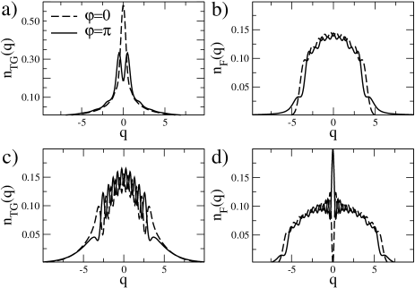
Figure 6: Interference in momentum space, $N=10$, a $\varphi=\pi$ phase is imprinted for $y>0$ (solid line), $\varphi=0$ case (dashed line); (a) TG gas, (b) Fermi gas, (c) TG gas after parity-selective evaporation, (d) Fermi gas after parity-selective evaporation.

We consider a phase imprinting with $w(y)=\Theta(y)$. Under this phase imprinting, a remarkable difference arises between the momentum distribution of both dual systems. For a moderate $N$ the visibility of the interference fringes in the TG gas is reduced (see Fig. 6a) but in the fermionic case the pattern has been washed out completely (see Fig. 6b). For larger $N$ the visibility of the TG dip decreases. It is hence clear that the observation of such effect in any of these dual systems would be difficult, and we turn our attention to a closely related alternative approach.

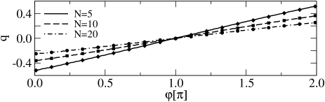
Figure 7: Displacement of the maximum of the momentum distribution as a function of the phase imprinted, for parity selective evaporation, fermionic cloud with only odd states. The symbols correspond to a smooth phase-imprinting profile with $\zeta=1/2$, whereas for the lines $\zeta=0$.

Recently, a parity-selective evaporation (PSE) method has been proposed which allows to prepare in principle excited states composed exclusively of odd-parity single-particle eigenstates dark06 . This is achieved by shinning a blue-detuned laser at $y\sim 0$ which removes the even-parity eigenstates. For a spin-polarized Fermi gas the excited many-body wavefunction becomes $\Psi_{F}(y_{1},\dots,y_{N})=\frac{1}{\sqrt{N!}}{\rm det}_{n,k=1}^{N}\psi_{2n-1}(y_{k})$. The corresponding momentum distribution exhibits a well-defined zero at $q=0$ for all $N$ which is stationary, and robust against significant smoothing of the phase-imprinting profile. The TG wavefunction equally follows from the Bose-Fermi map for PSE-prepared states. However, the $n_{TG}(q)$ is qualitatively insensitive to the selected parity of the single-particle states, and lacks any principal peak (or dip) potentially useful for momentum-space interferometry (see Fig. 6c). On the other hand, the pattern $n_{F}(q)$ in the fermionic case is reversed under phase imprinting, turning a zero into a peak in the momentum distribution (see Fig. 6d). Let us consider again a phase imprinting with the sigmoid profile (7). In Fig. 7 we have calculated the shift of the maximum in $n_{F}(q)$ as a function of $\varphi$ for the cases $\zeta=0$ (Heaviside function) and $\zeta=0.5$. The dependence is found to be linear even in the presence of the large smoothing in the profile $\zeta=0.5$.

Therefore, between both dual systems the TG gas is preferred using phase imprinting, whereas in combination with PSE, the fermionic system is a better candidate.

V Discussion

The localized phase imprinting method BS04 on trapped cold atoms has been discussed up to now mostly in connection with the generation and study of solitons. In this paper we have instead focused on the characterization of the momentum distribution right after the phase imprinting.

First, phase imprinting of half of the wavepacket can be regarded as a simple way to realize the interferometry in momentum space that has been previously put forward for more complex scattering processes between cold atoms an weak laser barriers PRL98 ; PRA01 ; PRA05 . Similar to the scattering setting, a central “dark notch” appears in the momentum distribution after phase imprinting, as well as an enhancement of the wings. An advantage with respect to the scattering method is that there is no need to make the width in momentum of the incident wave packet small to get the same transmission coefficient and therefore the same phase shift for all momenta. Thus we can make the trap tighter and tighter increasing the sensitivity.

Furthermore, the characterization of the momentum distribution is a preliminary step to determine the potential applicability of momentum interferometry where an unknown phase should be determined from the momentum shift of the central “dark notch”.

We have studied different configurations, regimes, and perturbations. The momentum dark notch for non-interacting particles in the ground state provides the most sensitive meter for the imprinted phase among the different states considered. In dimensionless units, the momentum shift of the “dark notch” versus the imprinted phase is in this case approximately given by $\tilde{q}_{0}=\sqrt{\frac{\pi}{2}}\frac{\varphi-\pi}{2}$ (see Eq. (4)). In dimensional units we get for the velocity

$$\tilde{v}_{0}=\sqrt{\frac{\hbar\omega}{m}}\left(\frac{\pi}{2}\right)^{3/2}\frac{\varphi-\pi}{\pi},$$

such that we can enhance the sensitivity concerning phase differences in principle to arbitrary high values by letting $\omega\to\infty$. If the external trap is immediately removed after the phase imprinting, the momentum distribution is essentially frozen and the velocity $\tilde{v}_{0}$ can be measured with standard time-of-flight technique. Assuming a free time of flight of duration $t$ after the phase imprinting the “dark notch” will move a distance $\tilde{s}_{0}=t\tilde{v}_{0}$. If we have a spacial resolution of $\Delta s$ then the resolvance $r$ of our momentum interferometer can be defined for the reference case as

$$r:=\frac{\pi}{\Delta\varphi}=\frac{t}{\Delta s}\sqrt{\frac{\hbar\omega}{m}}\left(\frac{\pi}{2}\right)^{3/2},$$

where $\Delta\varphi$ is the minimum resolvable deviation of the phase from $\pi$. For $t=200\,\mbox{ms}$, $m=$mass(⁸⁷Rb), $\omega=2\pi\times 2\,\mbox{kHz}$ and $\Delta s=5\mu{\mbox{m}}$, we get $r\approx 239$. The effects of unsharpness or spatial displacement of the phase jump have also been studied and the results qualitatively still holds. Many-body effects in the mean-field regime lead to a mild sensitivity loss but also to an interesting increase of visibility. In all cases there is still a linear dependence of the “dark notch” velocity on the phase $\varphi$, i.e. $v_{0}\approx\alpha\,(\varphi-\pi)$ such that the phase can be determined from the velocity of the “dark notch”.

Other extreme regimes, as the Tonks-Girardeau gas of Bosons or an ideal Fermi gas diminish the interference, except, in the later case, when an auxiliary parity-selection procedure is applied to retain odd-states. A peak is then formed with linear dependence on the imprinted phase, very stable with respect to the smoothness of the profile of the imprinting laser.

Finally, note that even though there are no atom-atom interactions in the reference case, some of the aspects usually attributed to the solitons may already be recognized, in particular the formation of the dark notch in momentum representation and its shift with the value of the phase jump or its smoothness. Dynamical studies of the state evolution will provide further comparison with soliton dynamics and will be dealt with elsewhere.

References

- (1) S. Brouard and J. G. Muga, Phys. Rev. Lett. 81, 2621 (1998).
- (2) A. L. Pérez Prieto, S. Brouard, and J. G. Muga, Phys. Rev. A 64, 012710 (2001).
- (3) A. Pérez Prieto, S. Brouard and J. G. Muga, Phys. Rev. A 71, 012703 (2005).
- (4) K. Bongs and K. Sengstock, Rep. Prog. Phys. 67, 907 (2004).
- (5) Ł. Dobrek, M. Gajda, M. Lewenstein, K. Sengstock, G. Birkl, and W. Ertmer, Phys. Rev. A 60, R3381 (1999).
- (6) B. P. Anderson, P. C. Haljan, C. A. Regal, D. L. Feder, L. A. Collins, C. W. Clark, and E. A. Cornell, Phys. Rev. Lett. 86, 2926 (2001).
- (7) M. D. Girardeau and E. M. Wright, Phys. Rev. Lett. 87, 050403, (2001).
- (8) I. Bloch et al., Nature 403, 166 (2000).
- (9) D.M. Gangardt and G.V. Shlyapnikov, Phys. Rev. Lett. 90, 010401 (2003).
- (10) M. Olshanii, Phys. Rev. Lett. 81, 938, (1998); V. Dunjko, V. Lorent, and M. Olshanii, ibid 86, 5413 (2001).
- (11) M.M. Cerimele, M.L. Chiofalo, F. Pistella, S. Succi, M.P. Tosi, Phys. Rev. E 62 (2000) 1382.
- (12) M.L. Chiofalo, S. Succi, M.P. Tosi, Phys. Rev. E 62 (2000) 7438.
- (13) G. Baym and C. J. Pethick, Phys. Rev. Lett. 76, 6 (1996).
- (14) F. Dalfovo, L. Pitaevskii, and S. Stringari, Physica Scripta, T66, 234 (1996).
- (15) A. Abramowitz and I. A. Stegun, Handbook of Mathematical Functions (Dover, New York, 1965)
- (16) M. Girardeau, J. Math. Phys. 1, 516, (1960).
- (17) M. D. Girardeau and E. M. Wright, Phys. Rev. Lett. 84, 5239 (2000).
- (18) A. M. Dudarev, M. G. Raizen, and Q. Niu, Phys. Rev. Lett. 98, 063001 (2007); A. del Campo and J. G. Muga, Phys. Rev. A 78, 023412 (2008).
- (19) R. Pezer and H. Buljan, Phys. Rev. Lett. 98 240403 (2007).
- (20) H. Buljan, K. Lelas, R. Pezer, and M. Jablan, Phys. Rev. 76, 043609 (2007).
- (21) H. Buljan, O. Manela, R. Pezer, A. Vardi, and M. Segev, Phys. Rev. A 74, 043610 (2006).