Axisymmetric smoothed particle hydrodynamics with self-gravity

Abstract

The axisymmetric form of the hydrodynamic equations within the smoothed particle hydrodynamics (SPH) formalism is presented and checked using idealized scenarios taken from astrophysics (free fall collapse, implosion and further pulsation of a sun-like star), gas dynamics (wall heating problem, collision of two streams of gas) and inertial confinement fusion (ICF, -ablative implosion of a small capsule-). New material concerning the standard SPH formalism is given. That includes the numerical handling of those mass points which move close to the singularity axis, more accurate expressions for the artificial viscosity and the heat conduction term and an easy way to incorporate self-gravity in the simulations. The algorithm developed to compute gravity does not rely in any sort of grid, leading to a numerical scheme totally compatible with the lagrangian nature of the SPH equations.

1 Introduction

Since the smoothed-particle hydrodynamics method was proposed by Gingold & Monaghan (1977) and Lucy (1977) thirty years ago it has become a powerful and very successful method, which is routinely used worldwide to model systems with complicated geometries. In particular the combination of the SPH method with hierarchical algorithms, addressed to efficiently organize data and calculate gravity, have led to a robust and reliable schemes able to handle complex geometries in three dimensions. In spite of these achievements little effort has been put in the development of axisymmetric applications of the method. However, a large body of interesting applications has to do with systems which have axisymmetrical geometry such as accretion discs, rotating stars or explosive phenomena (i.e. novae or supernovae events) provided the ignition takes place in a point-like region at the symmetry axis. The interaction between the gas ejected during a supernova explosion and the circumstellar matter has been extensively simulated using cylindric coordinates either with eulerian (Blondin et al., 1996) or SPH (Velarde et al., 2006) codes. In Inertial Confinement Fusion (ICF) studies the collapse of the deuterium capsule induced by laser ablation can be also approximated using two-dimensional hydrodynamics. Axisymmetrical hydrocodes are also useful to conduct resolution studies of three-dimensional codes just by imposing an initial configuration with the adequate symmetry. In these cases a comparison between the results obtained using the 3D-hydrocode and the equivalent, although usually better resolved, 2D simulation could help in numerical convergence studies. Several formulations of different complexity have been proposed to handle with the axisymmetric version of SPH. While the first algorithms were in general very crude, i.e. Herant & Benz (1992) and references therein, neglecting the so called hoop-stress terms, there were also more consistent SPH approximations, (Petscheck& Libersky, 1993). Recently more complete formulations were given by Brookshaw (2003) and by Omang et al. (2006). In particular the scheme devised by Omang et al. includes not only the hoop-stress terms but also a consistent treatment of the singularity line defined by the symmetry axis. The algorithm proposed by these authors relies in the use of interpolative kernels especially adapted to the cylindrical geometry. Although the resulting scheme is robust, being able to successfully pass several test cases, it has the numerical inconvenient that an elliptical integral has to be solved numerically at each integration step for each particle.

In this paper we propose a new formulation of the axisymmetric SPH technique which preserves many of the virtues stated by Brookshaw (2003) and Omang et al. (2006), being also able to handle the singularity axis in an efficient way. In our scheme there is no necessity to modify the interpolating kernel (we use the cubic spline polynomial). Instead, taking advantage of the symmetry properties across the Z-axis, we found several analytical correction factors to the physical magnitudes. These correction factors only affect particles moving at a distance from the Z-axis lesser than $2h$, being $h$ the smoothing-length parameter. For the remaining particles the SPH equations are identical to those given in Brookshaw (2003). In addition, we also give expressions for the artificial viscosity and a new heat conduction algorithm, which takes into account the hoop-stress contribution. Finally, we propose an original method to handle gravity within the SPH paradigm which is consistent with the gridless nature of that particle method. The text is organized as follows: the basic fluid equations written in axisymmetric coordinates, and corrected from axis effects when necessary, are provided in Section 2. In Section 3 we add useful physics to these equations consisting of an artificial viscosity term to handle shock waves (Section 3.1), an expression for thermal conduction (Section 3.2) and an algorithm addressed to calculate self-gravity within the axisymmetric hypothesis (Section 3.3). Section 4 is devoted to describe and discuss five test cases aimed at validating the proposed scheme. Finally the main conclusions of our work as well as some comments about the limitations of the developed scheme and prospects for the future are presented in Section 5.

2 Fluid equations in the axisymmetric approach.

An elegant approach to the axisymmetric Euler fluid equations was given by Brookshaw (2003) who derived the SPH form of these basic equations using the minimal action principle (see Monaghan 2005 and references therein for the history of variational SPH). The resulting expressions for mass, momentum and energy conservation written in the cylindrical coordinate system ${\mathbf{s}}=(r,z)$ are:

$$\eta_{i}=\sum_{j=1}^{N}m_{j}W_{ij}$$ (1)

$$\cases{\ddot{r}=2\pi\frac{P_{i}}{\eta_{i}}-2\pi\sum\limits_{j=1}^{N}m_{j}\left(\frac{P_{i}r_{i}}{\eta_{i}^{2}}+\frac{P_{j}r_{j}}{\eta_{j}^{2}}\right)\frac{\partial W_{ij}}{\partial r_{i}}\cr\cr\ddot{z}=-2\pi\sum\limits_{j=1}^{N}m_{j}\left(\frac{P_{i}r_{i}}{\eta_{i}^{2}}+\frac{P_{j}r_{j}}{\eta_{j}^{2}}\right)\frac{\partial W_{ij}}{\partial z_{i}}\cr\cr}$$ (2)

$$\frac{du_{i}}{dt}=-2\pi\frac{P_{i}~{}{v_{r_{i}}}}{\eta_{i}}+2\pi\frac{P_{i}~{}r_{i}}{\eta_{i}^{2}}\sum_{j=1}^{N}m_{j}(\mathbf{v_{i}-v_{j}})\cdot\mathbf{D}_{i}~{}W_{ij}$$ (3)

where $\eta_{i}=2\pi r_{i}\rho_{i}$ is the two-dimensional density of the i-particle, $\mathbf{v}=(v_{r},v_{z})$ its velocity, $W_{ij}=W_{ij}(\frac{|\mathbf{s_{i}-s_{j}|}}{h_{i}})$ the interpolating kernel and the remaining symbols have their usual meaning. The differential operator ${\mathbf{D}}=(\frac{\partial}{\partial r},\frac{\partial}{\partial z})$ is a cartesian operator written in the $(r,z)$  plane of cylindric coordinates. The first terms on the right in the r-component of equation (2) and equation (3) are called the hoop-stress terms. They are geometrical terms which arise from the nabla operator written in cylindrical coordinates. The smoothing-length parameter, $h$, is usually taken as the local resolution of the SPH. Equations (1), (2) and (3) along with the adequate equation of state (EOS) are the starting point to carry out numerical simulations of fluid systems with axisymmetric geometry. As boundary conditions we consider reflective ghost particles across the Z-axis and open flow at the outer limits of the system. For the $i$-particle with coordinates $(r_{i},z_{i})$ and velocity $(\dot{r}_{i},\dot{z}_{i})$ it is defined its reflective $k$-particle by taking $(r_{k},z_{k})=(-r_{i},z_{i})$, $(\dot{r}_{k},\dot{z}_{k})=(-\dot{r}_{i},\dot{z}_{i})$ and $m_{k}=m_{i}$. Thus position, velocity as well as other magnitudes such as density or internal energy of reflective particles are updated at each step not using the SPH equations but from the evolution of real particles. Even though the use of reflective boundary conditions is not strictly necessary in axisymmetric geometry it is useful to correctly represent the density and its derivatives near to the singularity axis.

2.1 Correction terms close to the singularity axis

One of the major causes of inaccuracy of axisymmetric SPH is the treatment of particles that get close to the symmetry axis. Unlike spherically symmetric systems where there is only one singular point, just at the center, here there is a singular line at $r=0$. A good treatment of particles moving close to the Z-axis is especially relevant for implosions such as the collapse of a self-gravitating system or in inertial confinement fusion studies. As far as we know only Omang et al. (2006) have consistently addressed this problem. In that paper the interpolation kernel is modified according to the particular geometry of the system, spherical or cylindrical. The resulting scheme does not have singularity problems when the particles approach the axis. However the resulting kernel does not have an analytical expression and must be calculated at any step for each particle using a numerical integration. Recently, useful fitting formulae were proposed by Omang et al. (2007) but still involving a large number of operations which slows the calculation.

An alternative way to handle with the symmetry axis, without modifying the basic SPH scheme given above, is to calculate correction terms to equations (1), (2) and (3), which become significant only close to the Z-axis. These correction factors arise because of the limited capability of standard kernels to interpolate accurately non linear functions. In the particular case of the two-dimensional density, $\eta=2\pi|r|\rho$, its profile is not longer linear in the axis neighbourhoods due to the presence of reflective particles. Usually the errors are small and the interpolation is precise to second order in $h$. Unfortunately, close to the symmetry axis errors grow and density and other physical magnitudes are not well reproduced, as it will be shown below. The detailed derivation of these corrections are given in Appendix A, leading to the following equations:

$$\widehat{\eta}_{i}=\sum_{j=1}^{N}m_{j}W_{ij}\times f_{1}^{i}=\eta_{i}\times f_{1}^{i}$$ (4)

where $\widehat{\eta}_{i}$ is the new, improved, two-dimensional density and $f_{1}^{i}$ is a correction factor which, for the cubic-spline kernel, reads (Appendix A):

$$f_{1}^{i}=\cases{\left[\frac{7}{15}\zeta_{i}^{-1}+\frac{2}{3}\zeta_{i}-\frac{1}{6}\zeta_{i}^{3}+\frac{1}{20}\zeta_{i}^{4}\right]^{-1}\qquad 0<\zeta_{i}<1\cr\cr\left[\frac{8}{15}\zeta_{i}^{-1}-\frac{1}{3}+\frac{4}{3}\zeta_{i}-\frac{2}{3}\zeta_{i}^{2}+\frac{1}{6}\zeta_{i}^{3}-\frac{1}{60}\zeta_{i}^{4}\right]^{-1}\cr\qquad\qquad\qquad\qquad{\mathrm{f}or}\qquad\qquad 1<\zeta_{i}<2\cr\cr 1\qquad\qquad\qquad\qquad\zeta_{i}>2\cr\cr}$$ (5)

being $\zeta_{i}=r_{i}/h_{i}$. A plot of $f_{1}(\zeta)$ and its first derivative is given in Fig. 1. Hereafter a hat will be placed over any corrected, and therefore, ”true” magnitude.

Figure 1: Plot of the correction factors $f_{1}$ and $f_{2}$ and their derivatives as a function of $\zeta=r/h$. The cubic spline interpolator kernel was assumed to compute $f_{1}$ and $f_{2}$ (Appendix A).

At this point it is useful to introduce a couple of algebraic rules:

$$\widehat{A}_{i}=\sum_{j}m_{j}\frac{A_{j}}{\widehat{\eta}_{j}}W_{ij}$$ (6)

$$\widehat{\eta A}_{i}=f_{1}^{i}\sum_{j}m_{j}A_{j}W_{ij}$$ (7)

which are valid as long as, close to the axis, the magnitude $A$ has a weak dependence in the r-coordinate. In particular, setting $A=1$  in equation (7) leads to equation (4).

To find the influence of the above correction factor in the momentum equation, equation (2), its is better to write the components of that equation in differential form. For the radial component we have:

$$\ddot{r}=-\frac{1}{\rho}\frac{\partial P}{\partial r}=-\frac{2\pi r}{\widehat{\eta}}\frac{\partial P}{\partial r}=2\pi\frac{P}{\widehat{\eta}}-\frac{2\pi rP}{\widehat{\eta}^{2}}\frac{\partial\widehat{\eta}}{\partial r}-\frac{\partial}{\partial r}\left(\frac{2\pi rP}{\widehat{\eta}}\right)$$ (8)

When $r\rightarrow 0$ the particle approaches the Z-axis where symmetry enforces the last term on the right to vanish for spherically symmetric kernels. The first term on the right is the hoop-stress term which should be exactly balanced by the central term when $r\rightarrow 0$, because the acceleration should be zero at the symmetry axis. Nevertheless, this does not happen unless the correction factor $f_{1}(\zeta)$ is taken into account during the calculation of the gradient of $\widehat{\eta}$:

$$\frac{\partial\widehat{\eta}}{\partial r}=\frac{\partial(f_{1}(\zeta)\eta)}{\partial r}=f_{1}(\zeta)\frac{d\eta}{dr}+\eta\frac{\partial f_{1}(\zeta)}{\partial r}$$ (9)

Similarly, for the Z-component in the momentum equation:

$$\ddot{z}=-\frac{1}{\rho}\frac{\partial P}{\partial z}=-\frac{2\pi r}{\widehat{\eta}}\frac{\partial P}{\partial z}=-\frac{2\pi rP}{\widehat{\eta}^{2}}\frac{\partial\widehat{\eta}}{\partial z}-\frac{\partial}{\partial z}\left(\frac{2\pi rP}{\widehat{\eta}}\right)$$ (10)

where now we simply have:

$$\frac{\partial\widehat{\eta}}{\partial z}=f_{1}(\zeta)\frac{\partial\eta}{\partial z}$$ (11)

The resulting momentum components in discrete SPH form can be obtained from equations (6) to (11):

$$\ddot{r}_{i}=2\pi\frac{P_{i}}{\widehat{\eta}_{i}}-2\pi\sum_{j=1}^{N}\left[m_{j}\left(\frac{P_{i}r_{i}}{\widehat{\eta}_{i}^{2}}\times f_{1}^{i}(\zeta_{i})+\frac{P_{j}r_{j}}{\widehat{\eta}_{j}^{2}}\right)\frac{\partial W_{ij}}{\partial r_{i}}\right]-$$

$$\left(\frac{2\pi P_{i}~{}r_{i}}{\widehat{\eta}_{i}\times f_{1}^{i}}\right)~{}\frac{df_{1}^{i}(\zeta_{i})}{dr_{i}}\qquad\qquad$$ (12)

$$\ddot{z}_{i}=-2\pi\sum_{j=1}^{N}m_{j}\left(\frac{P_{i}r_{i}}{\widehat{\eta_{i}}^{2}}\times f_{1}^{i}(\zeta_{i})+\frac{P_{j}r_{j}}{\widehat{\eta_{j}}^{2}}\right)\frac{\partial W_{ij}}{\partial z_{i}}$$ (13)

The value of pressure in equations (12) and (13) must be computed through the EOS using the ’corrected’ 3D-density, $\widehat{\rho}=\widehat{\eta}/(2\pi r)$.

Note that close to the axis the summatories in equations (12) and (13) are non symmetric with respect any pair of particles. Still the r-component of the momentum is conserved, even for those particles with $r<2h$, because of the imposed reflective boundary conditions. In the Z-axis the momentum is not exactly conserved within the band defined by $r<2h$. In general such loss is small, affecting a tiny amount of mass. In most of the tests described below total momentum was very well preserved.

A similar approach can be worked out to improve the energy equation:

$$\frac{du}{dt}=-2\pi\frac{P}{\widehat{\eta}}~{}v_{r}+2\pi\frac{Pr}{\widehat{\eta}^{2}}\frac{d\widehat{\eta}}{dt}$$ (14)

where:

$$\frac{d\widehat{\eta}}{dt}=\left[v_{r}\frac{\partial\widehat{\eta}}{\partial r}-\frac{\partial\widehat{(\eta v_{r})}}{\partial r}\right]+\left[v_{z}\frac{\partial\widehat{\eta}}{\partial z}-\frac{\partial\widehat{(\eta v_{z})}}{\partial z}\right]$$ (15)

being $\widehat{\eta}=\eta\times f_{1}$; $\widehat{(\eta v_{z})}=(\eta v_{z})\times f_{1}$ and $\widehat{(\eta v_{r})}=(\eta v_{r})\times f_{2}$. The factor $f_{2}$ is (Appendix A):

$$f_{2}^{i}=\cases{\left[\frac{14}{15}\zeta_{i}^{-1}+\frac{4}{9}\zeta_{i}-\frac{1}{15}\zeta_{i}^{3}+\frac{1}{60}\zeta_{i}^{4}\right]^{-1}\qquad 0<\zeta_{i}<1\cr\cr\big{[}-\frac{1}{45}\zeta_{i}^{-2}+\frac{16}{15}\zeta_{i}^{-1}-\frac{1}{3}+\frac{8}{9}\zeta_{i}-\frac{1}{3}\zeta_{i}^{2}+\frac{1}{15}\zeta_{i}^{3}-\cr\cr\qquad\frac{1}{180}\zeta_{i}^{4}\big{]}^{-1}\qquad\qquad\qquad\mathrm{for}\qquad 1<\zeta_{i}<2\cr\cr 1\qquad\qquad\qquad\qquad\zeta_{i}>2\cr\cr}$$ (16)

The resulting energy equation in discrete SPH form is:

$$\frac{du_{i}}{dt}=-2\pi\frac{P_{i}}{\widehat{\eta}_{i}}~{}v_{r_{i}}+2\pi\frac{P_{i}r_{i}}{\widehat{\eta_{i}}^{2}}\frac{d\widehat{\eta_{i}}}{dt}$$ (17)

where:

$$\frac{d\widehat{\eta_{i}}}{dt}=\sum_{j=1}^{N}m_{j}\left(f_{1}^{i}v_{r_{i}}-f_{2}^{i}v_{r_{j}}\right)\frac{\partial W_{ij}}{\partial r_{i}}+$$ (18)

(19)

$$\sum_{j=1}^{N}m_{j}\left(\frac{\partial f_{1}^{i}}{\partial r_{i}}v_{r_{i}}-\frac{\partial f_{2}^{i}}{\partial r_{i}}v_{r_{j}}\right)W_{ij}$$ (20)

(21)

$$+f_{1}^{i}\sum_{j=1}^{N}m_{j}\left(v_{z_{i}}-v_{z_{j}}\right)\frac{\partial W_{ij}}{\partial z_{i}}$$ (22)

Note that $f_{1}^{i}$, $f_{2}^{i}$ and their derivatives are only function of the current radial coordinate of the particle and its smoothing length. Thus, they can easily be computed and stored in a vector without introducing any significant computational overload. Examples about the use of the axisymmetric fluid equations with axis corrections, equations (4), (12), (13) and (17) in practical situations will be provided and discussed in Section 4.

3 Adding physics: Shocks, Thermal conduction and gravity

3.1 Artificial viscosity

As in three dimensions the treatment of shocks in the axisymmetric approach also relies in the artificial viscosity formalism. Nonetheless, there are a variety of artificial viscosity algorithms suited for SPH to choose at. We have adapted the standard recipe by Monaghan & Gingold (1983) to the peculiarities of the 2D-axisymmetric hydrodynamics. In that approach the artificial viscosity gives rise to a viscous bulk and shear pressure which is added to the normal gas pressure only in those regions where the particles collide (in the SPH sense). In three dimensions it is defined a magnitude, $\Pi_{ij}$:

$$\Pi_{ij}^{3D}=\cases{\frac{-\alpha_{0}\bar{c}_{ij}\mu_{ij}+\beta_{0}{\mu^{2}_{ij}}}{\bar{\rho}_{ij}}\qquad\qquad\qquad\mathbf{v_{ij}}\cdot\mathbf{r_{ij}}<0\cr\cr 0\qquad\qquad\qquad\qquad\qquad\quad\mathbf{v_{ij}}\cdot\mathbf{r_{ij}}>0\cr}$$ (23)

which is closely related to the viscous pressure. In equation (19) $\alpha_{0}$ and $\beta_{0}$ are constants of the order of unity, $\bar{\rho}_{ij}$ and $\bar{c}_{ij}$  are the average of density and sound speed of $i$ and $j$- particles, and $\mu_{ij}$ is:

$$\mu_{ij}=\frac{h_{ij}~{}\mathbf{v}_{ij}\cdot~{}\mathbf{r}_{ij}}{r^{2}_{ij}+\nu^{2}}$$ (24)

here $\mathbf{v}_{ij}=(\mathbf{v}_{i}-\mathbf{v}_{j})$, $\mathbf{r}_{ij}=(\mathbf{r}_{i}-\mathbf{r}_{j})$ and $\nu=0.1h$ avoids divergences when $r_{ij}\rightarrow 0$. The scalar magnitude $\Pi_{ij}$ has a linear and a quadratic term. The linear component mimics bulk and shear viscosity of fluids whereas the quadratic one is important to avoid particle interpenetration in strong shocks.

The easiest way to write the contribution of the artificial viscosity to the momentum and energy equations in an axisymmetric code is by changing the mass of the particles according to their distance to the Z-axis: $m\longrightarrow\frac{m}{2\pi r}$. The viscous acceleration becomes:

$$\mathbf{a}_{i}^{vis}=\sum_{j=1}^{N}\frac{m_{j}}{2\pi\bar{r}_{ij}}\Pi_{ij}^{3D}\mathbf{D}_{i}W_{ij}$$ (25)

Taking $\bar{\rho}_{ij}=\bar{\eta}_{ij}/(2\pi\bar{r}_{ij})$ in equation (19) the explicit dependence on $r_{ij}$  in the viscous acceleration formula is removed,

$$\mathbf{a}_{i}^{vis}=\sum_{j=1}^{N}m_{j}\Pi_{ij}^{(1)}\mathbf{D}_{i}W_{ij}$$ (26)

where $\Pi_{ij}^{(1)}$ is:

$$\Pi_{ij}^{(1)}=\cases{\frac{-\alpha_{0}\bar{c}_{ij}\mu_{ij}+\beta_{0}~{}\mu^{2}_{ij}}{\overline{\widehat{\eta}}_{ij}}\quad\mathbf{v_{ij}}\cdot\mathbf{s_{ij}}<0\cr\cr 0\qquad\qquad\qquad\quad\mathbf{v_{ij}}\cdot\mathbf{s_{ij}}>0\cr}$$ (27)

being $\mu_{ij}$:

$$\mu_{ij}=\frac{h_{ij}~{}\mathbf{v}_{ij}\cdot~{}\mathbf{s}_{ij}}{s^{2}_{ij}+\nu^{2}}$$ (28)

Expressions (22),(23) and (24) account for the cartesian part of viscosity. It has been shown (i.e. Monaghan 2005) that, in the continuous limit, these expressions become the Navier-Stokes equations provided shear and bulk viscosity coefficients are taken $\eta_{vis}=\rho\alpha_{0}hc/8$ and $\zeta_{vis}=5\eta_{vis}/3$ respectively. However, in cylindric geometry the stress tensor which appear in the Navier-Stokes equations also includes a term proportional to velocity divergence through the so called second viscosity coefficient. Therefore an extra term containing the magnitude $(v_{r}/r)$ must be added to $\Pi_{ij}^{(1)}$ to account for the convergence of the flux towards the axis. This new term, $\Pi_{ij}^{(2)}$, should fulfill a few basic requirements: 1) Far enough from the axis it should be negligible, 2) must vanish for those particles with $v_{r}\geq 0$, 3) for homologous contractions the viscous acceleration related to that term should be negligible, 4) it should be symmetric with respect particles $i$ and $j$ to conserve momentum. An expression satisfying the four items is:

$$\Pi_{ij}^{(2)}=\cases{\frac{-\alpha_{1}\bar{c}_{ij}q_{ij}+\beta_{1}~{}q_{ij}^{2}}{\overline{\widehat{\eta}}_{ij}}\quad v_{r_{i}}{\mathrm{and}}~{}v_{r_{j}}<0\cr\cr 0\qquad\qquad\qquad\quad{\mathrm{other~{}cases}}\cr}$$ (29)

where $q_{ij}=0.5~{}(\frac{h_{i}v_{r_{i}}}{r_{i}}+\frac{h_{j}v_{r_{j}}}{r_{j}})$. The resulting viscous acceleration is:

$$\mathbf{a}_{i}^{vis}=\sum_{j=1}^{N}m_{j}\Pi_{ij}^{2D}\mathbf{D}_{i}W_{ij}$$ (30)

where $\Pi_{ij}^{vis}=\Pi_{ij}^{(1)}+\Pi_{ij}^{(2)}$ Note that for a homologous contraction $v_{r}\propto r$ meaning $q\simeq\mathrm{const.}$, hence the gradient of $\left<\eta\Pi^{(2)}\right>$ vanishes fulfilling the third requirement above. In diverging shocks $\Pi_{ij}^{(2)}$ vanishes and only the cartesian part of viscosity matters. Therefore constants $\alpha_{0},\beta_{0}$ should remain close to their standard values $\alpha_{0}\simeq 1$ and $\beta_{0}\simeq 2$. All simulations presented in this paper were carried out using $\alpha_{1}=\alpha_{0}=1,~{}\beta_{1}=\beta_{0}=2$. In converging shocks, however, the effect of $\Pi_{ij}^{(2)}$ is to increase artificial viscosity introducing more damping in the system.

Equation (26), has the advantage that is formally similar to that used in three-dimensions. Therefore one can benefit from the well known features of the artificial viscosity in 3D, which can be directly translated to the axisymmetric version (several useful variations of equation (19) can be found in Monaghan 2005 ). In particular, it is straightforward to write the corresponding energy equation:

$$\left(\frac{du_{i}}{dt}\right)_{vis}\ =\frac{1}{2}\sum_{j=1}^{N}m_{j}\Pi^{2D}_{ij}(\mathbf{v_{i}-v_{j}})\cdot\mathbf{D}_{i}W_{ij}$$ (31)

which has to be added to the right hand of equation (3).

3.2 An approach to the conduction term.

The differential equation describing the evolution of the specific internal energy due to conductive or diffusive heat transfer is:

$$\left(\frac{du}{dt}\right)_{cond}=\frac{1}{\rho}\mathbf{\nabla}\cdot(\kappa\mathbf{\nabla}T)$$ (32)

being $\kappa$ the conductivity coefficient which in turn is a function of the local thermodynamic state of the material. The main difficulty to write equation (28) in a discrete equation suitable to SPH calculations is the existence of a second derivative. It is well known that second and higher order derivatives often pours a lot of numerical noise in disordered systems. A way to avoid that shortcoming is to reduce one degree the order of the derivative by taking the integral expression of equation (28), Brookshaw (1985) . It has been shown (see, for example, Jubelgas et al. (2004)) that in 3D-cartesian coordinates the following expression allows to approximate a second derivative using only the first derivative of the interpolation kernel:

$$\left(\nabla^{2}Y\right)_{i}=2\sum_{j=1}^{N}\frac{m_{j}}{\rho_{j}}\frac{Y_{j}-Y_{i}}{r_{ij}^{2}}\mathbf{r}_{ij}\cdot\mathbf{\nabla_{i}W_{ij}}$$ (33)

where $Y$ represents any scalar magnitude and $\mathbf{r}_{ij}=\mathbf{r}_{i}-\mathbf{r}_{j}$. An useful algebraic relationship which allows to write the heat transfer equation in SPH notation is:

$$\mathbf{\nabla}\cdot(\kappa\mathbf{\nabla T})=\frac{1}{2}\left[\nabla^{2}(\kappa T)-T\nabla^{2}\kappa+\kappa\nabla^{2}T\right]$$ (34)

Combining equations (29) and (30) the usual form of the heat transfer equation used in 3D-SPH studies is obtained. A mathematical expression for the heat transfer equation in axisymmetric SPH was given by Brookshaw (2003). However in the derivation of equation (29) there was not taken into account the $\simeq 1/r$  term which naturally arises whenever the divergence of a vector is estimated in cylindric coordinates:

$$\mathbf{\nabla}\cdot(\mathbf{\nabla}Y)=\frac{\left(\frac{\partial Y}{\partial r}\right)}{r}+\frac{\partial}{\partial r}\left(\frac{\partial Y}{\partial r}\right)+\frac{\partial}{\partial z}\left(\frac{\partial Y}{\partial z}\right)$$ (35)

It will be shown in Section 4.1 how the inclusion of the first term on the right of equation (31) improves the quality of the results in a particular test.

To obtain the adequate numerical approximation to equation (28) in axisymmetric SPH we first make use of equation (30):

$$\left(\frac{du}{dt}\right)_{cond}=\frac{1}{2\rho}\left\{\nabla^{2}(\kappa T)-T\nabla^{2}\kappa+\kappa\nabla^{2}T\right\}$$ (36)

Then, using equation (31) to develop each term inside the brackets and using the 2D-operator $\mathbf{D}\equiv(\frac{\partial}{\partial r},\frac{\partial}{\partial z})$  instead of $\mathbf{\nabla}$ the following expression is obtained:

$$\left(\frac{du_{i}}{dt}\right)_{cond}=\frac{1}{2\rho}\left\{\frac{1}{r_{i}}\frac{\partial(\kappa T_{i})}{\partial r_{i}}-\frac{T_{i}}{r_{i}}\frac{\partial\kappa_{i}}{\partial r_{i}}+\frac{\kappa_{i}}{r_{i}}\frac{\partial T_{i}}{\partial r_{i}}\right\}+$$ (37)

(38)

$$\frac{1}{\rho_{i}}\sum_{j=1}^{N}\left(m_{j}\frac{\kappa_{i}+\kappa_{j}}{\widehat{\eta}_{j}}(T_{i}-T_{j})\frac{\mathbf{s}_{ij}}{s_{ij}^{2}}\cdot\mathbf{D}_{i}W_{ij}\right)$$ (39)

The magnitudes inside the brackets are the new terms related to the hoop-stress. In order to calculate the derivatives we make use of one of the golden rules of SPH (Monaghan 2005 ):

$$\frac{\partial C_{i}}{\partial r_{i}}=\sum_{j}\frac{m_{j}}{\widehat{\eta}_{j}}(C_{j}-C_{i})\frac{\partial W_{ij}}{\partial r_{i}}$$ (40)

After a little algebra the following expression is obtained:

$$\left(\frac{du_{i}}{dt}\right)_{cond}=-\pi\sum_{j=1}^{N}m_{j}\frac{(\kappa_{i}+\kappa_{j})}{\widehat{\eta}_{i}\widehat{\eta}_{j}}(T_{i}-T_{j})\frac{\partial W_{ij}}{\partial r_{i}}+$$ (41)

$$2\pi r_{i}\sum_{j=1}^{N}m_{j}\frac{(\kappa_{i}+\kappa_{j})}{\widehat{\eta}_{i}\widehat{\eta}_{j}}(T_{i}-T_{j})\frac{\mathbf{s}_{ij}}{s_{ij}^{2}}\cdot\mathbf{D}_{i}W_{ij}$$ (42)

The presence of $(T_{i}-T_{j})$  in the equation ensures that there is not heat flux between different parts of an isothermal system. Note that the presence of the $r_{i}$ multiplier in the second term on the right side of equation (35) does not ensure complete conservation of the heat flux. However the total energy losses in the numerical test below simulating a thermal wave evolution were negligible. Of course equation (35) can be symmetrized by taking the arithmetical mean $\bar{r}_{ij}$ instead of $r_{i}$ but in that case the evolution of the thermal wave was not so well reproduced. On another note equation (35) is compatible to the second principle of thermodynamics in the sense that heat always flows from high to low temperature particles. To demonstrate this let us take a pair of particles $i$ and $j$ so that $T_{i}>T_{j}$. The second term on the right becomes negative because the scalar product ${\bf s_{ij}\cdot D_{i}}W_{ij}$ is always negative. The first term on the right is negative for $r_{i}<r_{j}$ and positive for $r_{i}>r_{j}$. As the heat flow from particle $i$ must be negative the only trouble could come if $r_{i}>r_{j}$. Nevertheless, even in that case heat flux is still negative if $r_{i}/(r_{i}-r_{j})>1/2$ because the sign of the second term in equation (35) prevails. Thus $r_{i}/(r_{i}-r_{j})>1/2$ is a sufficient condition tho get the right sign of heat flux between any pair of particles. As $r_{i}-r_{j}\simeq h$ such condition is fullfiled in a large domain of the system. The exception could be the axis vicinity where $r_{i}\rightarrow 0$. Nevertheless in that case symmetry enforces the heat flux to be negligible. Therefore we expect a good behaviour of the heat flux arrow although there are not excluded marginal violations if resolution is poor and strong heat fluxes were present close to $r=0$. A way to ensure complete compatibility to the second principle of thermodynamics is to make zero the flux between any pair of particles violating such principle.

3.3 Self-Gravity

Current 2D-hydrocodes often handle gravity by solving the Poisson equation or, if the system remains nearly spherical, by simply computing the enclosed lagrangian mass in a sphere below the point and using the Gauss law. Methods based on the Poisson solvers have proven very useful to find gravity in eulerian hydrodynamics where the same grid used to compute the motion of the fluid elements can be used in the calculation of gravity. However they have the difficulty to set suitable outer boundary conditions owing to the infinite range of the gravitational force. In lagrangian gridless methods such as SPH it is better to use the direct interaction among mass particles themselves to calculate gravity. The evaluation of the gravitational force through direct particle-particle interaction leads to an $N^{2}$ scheme that makes the computation feasible only for a limited number of particles. When $N$ is high, as it is frequent in three-dimensional calculations, one has to rely in approximate schemes such as those based in hierarchical-tree methods, Hernquist & Katz (1989). However hierarchical methods do not work efficiently in the 2D-axisymmetric approach because what we call particles are in fact rings of different size. Usually the ratio between the radius of these rings and the distance to the point where the force needs to be computed is too large to permit the multipolar approach to evaluate the gravitational force. Fortunately, the good resolution usually achieved in 2D using a moderate number of particles makes the direct calculation affordable.

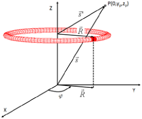
Figure 2: Sketch of the coordinate system and notation used to describe gravity.

According to Fig. 2 the gravitational force per unit of mass in a point P of coordinates $(0,y_{p},z_{p})$ (being Z the symmetry axis) due to the ring is:

$$\mathbf{g}(0,y_{p},z_{p})=G\int_{0}^{2\pi}\frac{\rho Rd\varphi}{(R^{2}+s^{\prime 2}-2y_{p}R\sin\varphi)^{3/2}}\times$$

$$\left[(R\sin\varphi-y_{p})~{}\mathbf{j}+(z-z_{p})\mathbf{k}\right]$$ (43)

where the meaning of the symbols is that shown in Fig. 2. The gravitational force acting onto the i-particle can be easily written as:

$$\mathbf{g_{i}}=\sum_{j=1}^{N}\frac{G}{2\pi}\frac{m_{j}}{(R_{j}^{2}+s_{i}^{\prime 2})^{3/2}}\times\qquad$$

$$\left[(R_{j}I_{1}-y_{i}I_{2})~{}\mathbf{j}+(z_{j}-z_{i})I_{2})~{}\mathbf{k}\right]$$ (44)

where $s_{i}^{\prime 2}=y_{i}^{2}+(z_{j}-z_{i})^{2}$, and $m_{j}=2\pi R_{j}\rho_{j}$ is the mass of the particle associated to the j-ring. Integrals $I_{1}$ and $I_{2}$ are defined as follows:

$$I_{1}=\int_{0}^{2\pi}\frac{\sin\varphi~{}d\varphi}{(1-\tau\sin\varphi)^{3/2}}$$ (45)

$$I_{2}=\int_{0}^{2\pi}\frac{d\varphi}{(1-\tau\sin\varphi)^{3/2}}$$ (46)

where the parameter $\tau$ is:

$$\tau=\frac{2y_{i}R_{j}}{R_{j}^{2}+s_{i}^{\prime 2}}$$ (47)

Although the elliptical integrals $I_{1}$ and $I_{2}$ can not be solved analytically they can be tabulated as a function of the parameter $\tau$ given by equation (40). It is straightforward to show that the value of $\tau$  is always inside the interval $\tau\epsilon[0,1)$, although for $\tau\rightarrow 1$ the integrals $I_{1}$ and $I_{2}$ become divergent. Therefore the gravity force can be calculated in an efficient way using the following recipe:

1) Build a table for $I_{1}$ and $I_{2}$ as a function of $\tau$. A table with $10^{4}$ rows with values $0\leq\tau\leq 0.9999$ evenly spaced is sufficient.

2) To increase the speed do not interpolate from that table but take just the row which is closest to the actual value of $\tau$ calculated using equation (40).

3) Note that parameter $\tau$ is symmetric with respect any pair of particles, $\tau_{i}=\tau_{j}$, thus $I_{1}(\tau_{i})=I_{1}(\tau_{j})$ and $I_{2}(\tau_{i})=I_{2}(\tau_{j})$. Therefore only half of the interactions have to be calculated.

If the algorithm is optimized the scheme is able to provide the exact value of the gravity for several dozens of thousand particles. In many applications using $\simeq 5~{}10^{4}$ particles in two-dimensions is enough to guarantee a good resolution.

Another physical magnitude of interest is the gravitational potential at the position of the i-particle. It is easy to show that the contribution of the j- ring to the gravitational potential is:

$$V_{i}=\frac{G}{2\pi}\frac{m_{j}}{(R_{j}^{2}+s_{i}^{\prime 2})^{1/2}}I_{3}$$ (48)

where,

$$I_{3}=\int_{0}^{2\pi}\frac{d\varphi}{(1-\tau\sin\varphi)^{1/2}}$$ (49)

Again the same recipe given above to compute the force can be used to efficiently calculate $V_{i}$. On the other hand the exact computation of the gravitational potential allows to calculate the gravitational force by taking the gradient of $V$ at any point.

$$\mathbf{g_{i}}=-(\mathbf{D}V)_{i}$$ (50)

A more suitable form for SPH calculations can be obtained using:

$$\widehat{\eta}\mathbf{D}V=\mathbf{D}(\widehat{\eta V)}-V\mathbf{D}\widehat{\eta}$$ (51)

which, according to equations (7) and (9), leads to the following discrete equation:

$$\mathbf{g_{i}}=-(\mathbf{D}V)_{i}=\frac{f_{1}^{i}}{\widehat{\eta}_{i}}\sum_{j=1}^{N}m_{j}(V_{i}-V_{j})\mathbf{D}_{i}W_{ij}+$$

$$\frac{\left(\frac{df_{1}^{i}}{dr}\right)}{\widehat{\eta}_{i}}\sum_{j=1}^{N}m_{j}(V_{i}-V_{j})W_{ij}~{}u_{r}$$ (52)

where $f_{1}$ is the corrective term given by equation (5) and $u_{r}$ the unit vector in the r-axis.

This second route to calculate the gravitational force is computationally more efficient than evaluating equation (37) because the gradient of the potential is a local quantity which can be calculated in the same part of the algorithm devised to compute the density or other magnitudes in the hydrocode. It has the additional advantage that the resulting force is smoothed by the SPH interpolation procedure avoiding divergences when a pair of particles become too close. In Fig. 5 (bottom-right) there are shown the gravity profile calculated using equation (45) (filled triangles) and the pressure gradient term (continuum line) along a sun-like polytropic structure. As it can seen the fit is satisfactory except at the surface where the pressure gradient is overestimated. Although using the potential to calculate gravity is not as exact as the direct force calculation it is a factor two faster because there is a lesser amount of numerical operations in the double loop of the gravity routine.

Needless to say, the simplicity of the proposed scheme makes the parallelization of the gravity computational module straightforward. In this case calculations with $10^{5}-10^{6}$ particles could become feasible even for desktop computers with multiple core processors.

3.3.1 Free-fall collapse of homogeneous gas structures. Rotation.

As an initial check of the gravity algorithm resulting from equation (45) we have simulated the free-fall collapse of a uniform density sphere of mass M₀ and radius R₀. It is a standard test which has the following analytical solution:

$$\frac{t}{t_{ff}}=1-\frac{2}{\pi}\left\{\sin^{-1}\left[\left(\frac{r}{r_{0}}\right)^{\frac{1}{2}}\right]-\left(\frac{r}{r_{0}}\right)^{\frac{1}{2}}\left(1-\frac{r}{r_{0}}\right)^{\frac{1}{2}}\right\}$$ (53)

where $r_{0}$ is the initial position of the fluid element and $0\leq t\leq t_{ff}$. The free-fall time $t_{ff}$ is:

$$t_{ff}=\frac{\pi}{2}\left(\frac{R_{0}^{3}}{2GM_{0}}\right)^{\frac{1}{2}}$$ (54)

We built an uniform sphere with M₀=1 M_☉ and R₀=R_☉ filled with $N=15396$ particles settled in a square lattice. Gas pressure and artificial viscosity were set to zero so that the structure collapsed under gravity force. Afterwards the implosion was followed until the elapsed time was close to $t_{ff}$. Although restricted to spherical symmetry the free-fall test is quite demanding because the evolution is highly non linear, allowing for a good check of both the gravity module and the integration scheme (see next section for details). In Fig. 3 there is represented the evolution of a particle initially located at $r_{0}=2/3~{}R_{\sun}$. As we can see its evolution is in good agreement to the analytical solution given by equation (46).

Figure 3: Free-fall test. Triangles represent the analytical solution in each case. The initial radius of the particle was $r_{0}=2/3~{}R_{\sun}$, $z_{0}=0$ in all cases.

A question of great interest in astrophysics is the capability of axisymmetric SPH codes to handle rotation. The topic is far from trivial because in general it involves transport of angular momentum via viscous coupling. Even though a complete answer to that question is beyond the scope of the present work there is a particular case that can be handled with the present scheme: the fast implosion (or expansion) of a self-gravitating rotating cloud. If the characteristic dynamical time is much shorter that the viscous coupling time we can impose angular momentum conservation around the symmetry axis to solve this problem. The strategy is simply to add the centrifugal force which arises from finite angular momentum to the r-component of gravity. As an example we have simulated the collapse of a slender rotating cylinder of gas with uniform density centered at the coordinate origin. The initial conditions are specified by the mass $M_{cyl}$ the radius $R_{cyl}$ and the length of the cylinder $Z_{cyl}$. If we suppose rigid rotation the specific angular momentum of a mass point is given by $L_{z}(r_{0})=w_{0}~{}r_{0}^{2}$ being $w_{0}$ the initial angular velocity of the cylinder and $r_{0}$ the position of the fluid element at the initial time $t_{0}$. Angular momentum conservation demands $L_{z}(r,t)=L_{z}(r_{0})$ so that the centrifugal force is $F_{c}=L_{z}^{2}(r_{0})/r^{3}(t)$ which is added to the first component of gravity, calculated using equation (45), to obtain an effective gravity value. As in the case of the spherical collapse we have taken $M_{cyl}=M_{\sun}$ and $R_{cyl}=R_{\sun}$ while the cylinder length was $Z_{cyl}=20R_{cyl}$. The evolution of mass points were followed assuming two values for the angular momentum: 1) zero angular momentum and 2) $L_{z}(r_{0})=\sqrt{(0.5g_{0}r_{0}^{3})}$ where $r_{0}=2/3~{}R_{cyl}$ for which centrifugal force was a half of gravitational force at that position. In this case we have used a larger number of particles, $N=70000$  to reduce boundary effects.

On the other hand, assuming $Z_{cyl}>>R_{cyl}$ and using the Gauss-law it is possible to work out an analytical approach to the above scenario. The acceleration equation becomes:

$$\ddot{r}=-g_{0}\frac{r_{0}}{r}+\frac{L_{0}^{2}}{r^{3}}$$ (55)

where $L_{0}\equiv L_{z}(r_{0})$ and $g_{0}$ is the value of gravity at $r=r_{0}$. According to the Gauss-law $g_{0}=2GM_{cyl}~{}r_{0}/(R_{cyl}^{2}~{}Z_{cyl})$, but it is better to take $g_{0}$ directly from the SPH simulation to ensure identical initial conditions in both calculations. The solution of equation (48) is:

$$t(r)=-\int_{r_{0}}^{r}\frac{dr^{\prime}}{\left[-2g_{0}r_{0}\ln\frac{r^{\prime}}{r_{0}}+L_{0}^{2}\left(\frac{1}{r_{0}^{2}}-\frac{1}{r^{\prime 2}}\right)\right]^{\frac{1}{2}}}$$ (56)

which has to be solved numerically once $r_{0}$ and $L_{0}$ are specified.

Fig. 3 depicts the evolution of a particle initially located at $r_{0}=2/3~{}R_{cyl},Z_{0}\simeq 0$ without and with initial angular momentum as well as that obtained using the the analytical approach, equation (49). The case with zero angular momentum led to the free fall of the mass element which was less violent than the spherical case owing to the lower initial density in the cylinder. As it can be seen in Fig. 3 the agreement between analytical and SPH results is not as good as in the spherical case for $t>t_{ff}$. This is not surprising because boundary effects at cylinder edges progressively affects gravity at current particle test position and its evolution is very sensible to small variations of gravity force.

When angular momentum was added to the cylinder at $t_{0}=0$ s the implosion of the structure slowed down. As commented above the amount of angular momentum was chosen to get a centrifugal force contribution at $r_{0}=2/3~{}R_{cyl}$  equal to a half of gravity force at that position. As we can see in Fig. 3 the result of the simulation is in better agreement to the analytical approach than the pure free-fall case. This is because the evolution is driven not only by gravity and errors due to the finite size of the rotating cylinder are not affecting so much the outcome as in the non rotating case. At $t\simeq 5$ t_ff the fluid element begins to be centrifugally sustained, in good match to the analytical estimation.

4 Test cases

In this section we describe and discuss in detail five test cases addressed to validate the computational scheme developed in the precedent sections. The first test involves the propagation of a thermal discontinuity born at the symmetry axis. It is a well known calculation which has an analytical solution to compare with. Three calculations: the gravitational collapse of a polytrope, the implosion of a homogeneous capsule, and the wall shock problem deal with implosions of spherically symmetric systems. Although, at first glance, such constraint looks too restrictive in fact it is not, because the spherical symmetry is not a natural geometry for axisymmetrical systems described with cylindrical coordinates. Any deviation from the pure spherical symmetry during the implosion will trigger the growth of hydrodynamical instabilities. Therefore the preservation of the symmetry during the calculation is an important feature to be added to mass, momentum and energy conservation. Finally the last test was devoted to simulate the collision of two bubbles of fluid along the Z-axis.

The initial models were calculated by mapping the spherically symmetric profiles into a 2D distribution of particles settled in a square lattice. The mass of the particles was conveniently adjusted to reproduce the density profile of the one-dimensional model. For example, masses proportional to the $r-$coordinate of the particle were taken to obtain models with constant density. Reflective boundary conditions using specular ghosts particles were imposed across the Z-axis. The EOS was that of an ideal gas with $\gamma=5/3$ and radiation in the test devoted to the collapse of a polytrope, and only gas ideal for the other tests. We have used and adaptive smoothing length parameter $h(\mathbf{s},t)$ which was updated at each time step to keep a constant number of neighbours $n_{v}=36$ within a circle of radius $2h$. The interpolating kernel was the cubic polynomial spline. Numerical integration of SPH fluid equations was performed using a two-step centered scheme with second order accuracy. It is worth to mention that in the free-fall test of a homogeneous sphere the velocity was updated using the XSPH variant of Monaghan (1989) to avoid particle penetration through the symmetry axis. In this particular test mass points at low radius are proner to cross Z-axis because pressure and viscous forces were artificially set to zero. Therefore any residual value of gravity can impel particles located close to the center towards unphysical $r<0$ values. We have updated only the $r$-component of velocity using the following expression:

$$\tilde{\dot{r}_{i}}=\dot{r}_{i}+\epsilon~{}2\pi~{}r_{i}\sum_{j=1}^{N}\frac{m_{j}}{\widehat{\eta}_{ij}}\left(\dot{r}_{j}-\dot{r}_{i}\right)~{}W_{ij}$$ (57)

where $\tilde{\dot{r}_{i}}$ is the new, smoother, velocity. The parameter $\epsilon$ was taken variable:

$$\epsilon=\cases{\epsilon_{0}\left(1-\frac{\left(\frac{r}{h}\right)^{2}}{9}\right)\qquad\qquad r\leq 3h\cr 0\qquad\qquad\qquad r>3h\cr}$$ (58)

where $\epsilon_{0}=0.5$. Using XSPH variant to move particles enforces $\dot{r}\rightarrow 0$ when $r\rightarrow 0$, making it difficult for particles to cross the axis.

4.1 Evolution of a thermal discontinuity

Lets consider the problem relative to the propagation of a thermal wave moving through an uniform static medium. This is a well known test, addressed to check the capability of the numerical scheme to handle thermal discontinuities. The initial model was a sample of 57908 particles evenly distributed in a square lattice so that the density was $\rho=1$ g.cm^-3. A $\delta$-like jump in internal energy originates a a thermal wave front which evolves according to:

$$u(r,z,t)=\frac{A}{(4\pi c_{v}kt)^{\frac{3}{2}}}\exp\left(-\frac{r^{2}+z^{2}}{4c_{v}kt}\right)+u_{0}$$ (59)

where $c_{v}$ is the specific heat and $k$ is the thermal conductivity. The following set of values were taken: $A=10^{5}$ ergs.cm³/g, $u_{0}=10^{3}$ erg.g^-1 and $c_{v}k=1$ cm².s^-1. The initial internal energy profile was that given by equation (52) for $t=1$ s, which was taken as the initial time (t=0 s) for the SPH simulation. The evolution of the thermal signal is then controlled by the heat conduction equation, equation (35).

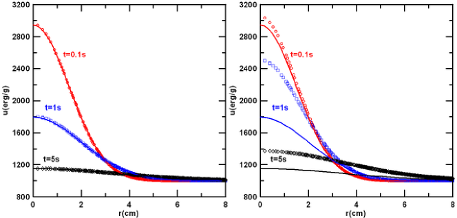
Figure 4: Evolution of a thermal discontinuity initially seeded around the symmetry axis. The profile of the internal energy at different times is well reproduced by the SPH when the hoop-stress term is included (left). However when that term is neglected the result does not match the analytical solution represented by the continuum line (right).

In Fig. 4 (left) there is represented the thermal profile at different times. As we can see the coincidence with the analytical solution given by equation (52) is excellent. As time goes on the peak of the signal and its slope decreases due to heat diffusion. The initial discontinuity is rapidly smeared out by thermal diffusion and soon a thermal wave is born which travels to the right, equalizing the internal energy of the system. At t=5 s the profile of the internal energy of the gas is already quite flat and the system is not far from thermal equilibrium. At that moment total energy was conserved up to $5~{}10^{-5}$. In Fig. 4 (right) it is shown the evolution of the thermal profile which results when the first term on the right side in equation (35) is removed. As we can see the evolution is no longer reproduced by the SPH calculation. Therefore it is of utmost importance to include that term, especially in those calculations dealing with strong thermal gradients close to the symmetry axis.

4.2 Gravitational collapse of a polytrope

The second test involves a catastrophic, albeit highly unprobable, astrophysical scenario. A spherically symmetric sun-like polytrope was suddenly unstabilized by removing the $20\%$ of its internal energy so that the structure collapsed under the gravity force. At some point the collapse is halted and an accretion shock forms which manages to eject part of the mass of the polytrope. Several episodes of recontraction followed by mass loss ensued until the star sets in a new equilibrium state. Even though that particular scenario is not realistic it contains several pieces of physics of great interest because accretion shocks and pulsational instabilities are ubiquitous in astrophysics. As the initial model has spherical symmetry we expect it to be preserved during the implosion and further bounce. The conservation of the symmetry is a demanding test for multidimensional hydrocodes in those cases where there are episodes of strong decelerations. In the particular case of axisymmetric hydrodynamics the higher numerical noise close to the symmetry axis may trigger the growth of convective instabilities. An additional advantage of considering an spherically symmetric initial model is that the evolution calculated with the SPH code can be checked using standard lagrangian hydrodynamics in one dimension.

Figure 5: Density, gravity and pressure gradient profiles of the polytrope. Upper-left and right: density profile without and with axis corrections respectively. Bottom-left and right: the same but for the pressure gradient. The absolute value of gravity computed using the gradient of the gravitational potential calculated using equation (45) is marked with full triangles (bottom-right). All mass points of the polytrope have been represented. Neglecting axis corrections leads to a much larger dispersion in the profiles.

The initial model was a $1$ M_☉ spherically symmetric polytrope of index $n=3$. The radius was set equal to $1$ R_☉ so that the central density was $\rho_{c}=77$ g.cm^-3 . Once the 1D equilibrium model was built it was mapped to a 2D distribution of 51408 particles located in a rectangular lattice. The mass of the particles were conveniently adjusted to reproduce the density profile of the polytrope. In Fig. 5 there are shown the profiles of density and gradient of pressure at t=0 s calculated using the 2D-SPH. As we can see the inclusion of the corrective term $f_{1}$ given by equation (5) in the momentum equation is crucial to get good enough profiles of these quantities to guarantee the stability of the initial model. The polytrope was perturbed by reducing the temperature everywhere in a 20% of its equilibrium value. Afterwards the evolution was followed with the 2D-SPH from the implosion until the first pulsation and compared to that obtained by a 1D lagragian hydrocode. The main features of the model and a summary of the results are shown in Table 1.

Table 1: Main features of test models described in Sections 4.2 and 4.3. Conservation of momentum is given by the center of mass displacement $\Delta\bar{r}=\left[(\bar{r}(t)-\bar{r}_{0})-\bar{v}_{r}^{0}t\right]$  and $\Delta\bar{z}=\left[(\bar{z}(t)-\bar{z}_{0})-\bar{v}_{z}^{0}t\right]$  divided by the radius of the configuration at that time (columns 5 and 6). Momentum and energy conservation correspond to the last calculated model shown in Figs. 6, 7, 8 and 9.

Test	Number of Part.	$\left(\frac{\rho_{max}}{\rho_{0}}\right)_{1D}$	$\left(\frac{\rho_{max}}{\rho_{0}}\right)_{2D}$	$\frac{|\Delta\bar{r}|}{R}$	$\frac{|\Delta\bar{z}|}{R}$	$\frac{|\Delta E|}{E_{0}}$
Polytrope	51408	2.43	2.49	$5~{}10^{-15}$	$10^{-11}$	$5~{}10^{-3}$
Capsule implosion	30448	29	32	$4~{}10^{-14}$	$10^{-11}$	$8~{}10^{-3}$
Noh test	50334	64	58	$6~{}10^{-14}$	$3~{}10^{-8}$	$2~{}10^{-3}$
Gas clouds collision	55814	-	-	$5~{}10^{-14}$	$1.3~{}10^{-3}$	$10^{-2}$

Soon after the model was destabilized the polytrope started to collapse. At t$=960$ s a maximum of the central density $\rho_{max}=192.8$ g.cm^-3was reached. A similar maximum of $\rho_{max}=187.1$ g.cm^-3was obtained using one-dimensional hydrodynamics. The profiles of density and radial velocity at different times are depicted in Fig. 6. As we can see the evolution calculated in one and two dimensions is very similar and, in general, both profiles are in good agreement. At our last calculated time, t$=1545$ s, the shock is already breaking out the surface of the polytrope. Shortly after that time some mass is ejected from the surface and, as the 1D calculation shows, the star embarks in a long pulsational stage until a new equilibrium state is achieved.

Therefore the numerical scheme was able to handle with this scenario. The algorithm devised to calculated the gravity using equation (45), which relies in the direct interaction between rings (Fig. 2), did a good job. The artificial viscosity module was also able to keep track with the shocks although, at some stages, the post-shock region showed a small amount of spurious oscillations. These numerical oscillations in the velocity profile are clearly visible in Fig. 6 at t$=1545$ s. In the last three columns of Table 1 there is information concerning momentum and energy conservation at t$=1545$ s, our last calculated model. There was an excellent momentum conservation, close to machine precision, whereas the conservation of energy was more modest, $\simeq 0.5\%$. On the other hand the spherical symmetry was also quite well preserved during the calculation. On the negative side we find that the two-dimensional calculation was systematically delayed with respect its one-dimensional counterpart. The relative shift in time remained approximately constant, around $1,5$%, during the evolution. For the sake of clarity the elapsed times shown in Fig. 6 were that of the SPH simulation and the times of the one-dimensional evolution were conveniently chosen to fit the 2D profiles.

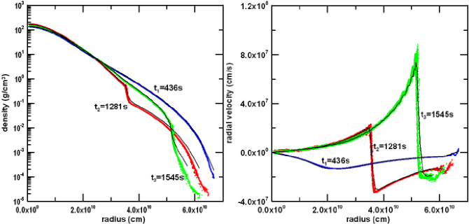
Figure 6: Density profile (left) and radial velocity (right) during the implosion and further rebound of the polytrope at different times. The black continuum line is the profile calculated using a one-dimensional hydrocode of similar resolution. At t=1545 s the shock wave is breaking the surface of the star. In the figure all particles used during the calculation are shown.

4.3 Implosion of a homogeneous capsule

Probably the most unfavourable case to numerical simulation is that of a strong implosion as it currently appears, for example, in ICF studies. Thus, our third test deals with the implosion of a homogeneous spherical capsule of size $R_{0}=1$  cm and density $\rho_{0}=1$ g.cm^-3, induced by the (artificial) ablation of its surface. The ablation of the capsule was triggered by the instantaneous deposition of energy in the outermost layers of the capsule, which had their internal energy increased in the same proportion. The energy deposition profile was taken linear from $s=0.8$ cm to $s=R_{0}=1$ cm so that the internal energy at $R_{0}=1$ cm was a factor $10^{4}$ higher than that at s=0.8 cm. Below s=0.8 cm a flat profile of the internal energy was assumed. The rocket effect caused by the evaporation of the surface layers forms a strong shock wave which compresses the interior of the capsule. The convergence of the shock at the center of the sphere increases the temperature and the density in a large factor, much larger than that obtained in the previous section dealing with the collapse of a solar-like polytrope. The main features of the model are shown in Table 1 and Fig. 7. The profiles of density and radial velocity at several times are depicted in Fig. 7 which also shows the profiles obtained using a 1D-lagrangian hydrocode (continuum lines) with the same physics and identical initial conditions. The evolution of the capsule can be summarized as follows. Soon after the initial energy deposition a pair of shock waves moving in opposite directions appear (profiles at t=0.0044 s in Fig. 7). As the reverse shock approaches the center it becomes stronger owing to the spherical convergence (profiles at t=0.0087 s in Fig. 7). Once the maximum compression point is reached, $\rho_{max}=31$ g.cm^-3at t$=0.0111$  s, the wave reflects. When t=0.0150 s the density peak has already dropped to 7 g.cm^-3and most of the material of the capsule is expanding homologously. At t=0.0264 s the reflected wave reaches the initial radius of the capsule, $R_{0}=1$ cm. At that time the material of the capsule is rather diluted $\rho(r)<<1$ g.cm^-3and the radial velocity profile consist of two homologously expanding zones separated by a transition region at $s\simeq 1$ cm. At the last calculated time, t$=0.0264$  s, the outermost layer of the sphere has expanded until $s=10$ cm, ten times the original size of the capsule. As we can see the 2D-simulation match quite well the 1D results. According to Table 1 the central density at the moment of maximum compression is almost the same in both calculations. The conservation of momentum is very good, close to machine precision (columns 5, 6 of Table 1), while numerical energy losses remained lesser than 1% (last column in Table 1). However, an inspection of Fig. 7 reveals that the spherical symmetry was not so well preserved as in the collapsing polytrope. Now the implosion of the capsule was more violent and the deceleration phase before the bounce was more intense, making easier the growth of instabilities. Even though the initial model had good spherical symmetry, the initial distribution of the particles in a regular lattice acts as a source of the so called hour-glass instability. Such instability is related to the existence of preferred directions along the grid through which the stress propagates. As in the previous test another point of conflict between the 1D and the 2D calculations is that the 2D evolution is a bit delayed with respect its one-dimensional counterpart. For instance, the times at which the maximum central densities are achieved are $t_{1D}=0.01095$ s and $t_{2D}=0.0111$ s, so that the relative difference was around $1-2$%. Such percent level of discrepancy remained approximately constant during the calculation.

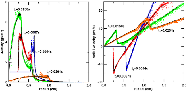
Figure 7: Same as in Fig. 6 but for the small capsule implosion.

4.4 Wall heating shock: the Noh test

The wall heating shock test, Noh (1987), was especially devised to analyze the performace of algorithms addressed to capture strong shocks. Basically the wall heating shock test consists in making a sphere or a cylinder implode by imposing a converging velocity field. For these geometries there is an analytical approach to the evolution of density and thermodynamical variables as a function of the initial conditions. The results of numerical codes can be compared with the analytical solution to seek the best method or to choose for optimal combination of parameters. It is well known that schemes which rely in artificial viscosity have difficulties to handle the wall heating shock test. The reason is that artificial viscosity spreads the shock over a 3-4 computational cells, which induces an unphysical rise of internal energy ahead the shock. In the case of spherical or cylindrical geometry the artificial increase in internal energy is magnified by the geometrical convergence of the shock. Therefore the wall shock problem represents a strong challenge for the axisymmetric SPH. Brookshaw (2003) carried out a similar test with the SPH code but far from the symmetry axis. In particular he modelled the impact of two supersonic streams of gas, obtaining good profiles for density and internal energy except in a small region around the collision line. The density profile showed a dip at that region while a large spike was seen in the internal energy. Both, the dip and the spike are numerical artifacts which can be smoothed out by using an artificial heat conduction term to spread the excess of internal energy and reduce the error around the contact discontinuity.

To check the performance of our code we have settled N=50334 particles in a square lattice. As in the previous tests the mass of the particles was conveniently crafted to reproduce an spherical homogeneous system with initial radius $R_{0}=1$ cm. The initial conditions were taken as in Noh (1987): $\rho(s,0)=1$ g.cm^-3; $\dot{s}(s,0)=-1$  cm.s^-1; $u(s,0)=0$ erg.g^-1. The exact solution at time t=0.6 s for $\gamma=5/3$ is shown in Fig. 8 (dashed line). The analytical profile is characterized by a constant post-shock state until distance $s=0.2$ cm followed by a rapid decrease in density and internal energy. In the shocked zone density reach a constant value $\rho=64$ g.cm^-3while internal energy was $u=0.5$ erg.g^-1. The combination of such harsh initial conditions plus geometrical convergence leads to an strong implosion, even harder than that described in the ablated capsule test. In Fig. 8 (left) there are shown the spherically averaged profiles of density and internal energy obtained using SPH at t$=0.6$ s. The error bars in the plot give the $1\sigma$ dispersion of these variables with respect its mean value in the shell. As we can see the resulting profiles compare poorly with the analytical results in the shocked region. In addition the dispersion is high, especially at low radius, a clear signature for the presence of numerical noise. Close to the axis there is the typical artificial combination of a dip (in density) and spike (in internal energy). The maximum density value was $\rho\simeq 58$ which is around 10% lower than the exact value. Such bad quantitative agreement was not unexpected because it is common to all hydrodynamic codes which use the artificial viscosity scheme. A way to improve the quality of the simulation is to allow for heat conduction in the hydrocode to remove the thermal energy spike and to sharpen the shock. Recipes to obtain an artificial conductivity coefficient in SPH to better handle the wall shock problem were given by Monaghan (1992) and Brookshaw (2003). For this calculation we have adapted the recipe of Monaghan to the features of the axisymmetric SPH defining an artificial conductivity for the i-particle:

$$k_{i}=\bar{\rho}_{ij}~{}\bar{c}_{v_{ij}}\bar{h}_{ij}\left(\bar{c}_{ij}+4|\mu_{ij}|\right)$$ (60)

where $\bar{c}_{v_{ij}}$ is the symmetrized specific heat and $|\mu_{ij}|$  is the artificial viscosity parameter given by equation (24). According to equation (53) $k_{i}=k_{j}$, which can be used directly in equation (35) to compute the artificial heat flux. As shown in Fig. 8 (right) the inclusion of the artificial heat conduction term leads to a significant improvement of the results. Not only the profound dip in density in the central region has been removed but the simulation shows much lesser dispersion around the averaged values of density and internal energy. However the maximum peak in density still remains $\simeq 10\%$ below the theoretical value. In this respect the only way to improve the results is sharpening the shock either by using adaptive kernels, Owen et al. (1998), Cabezón et al. (2008), or by increasing the number of particles.

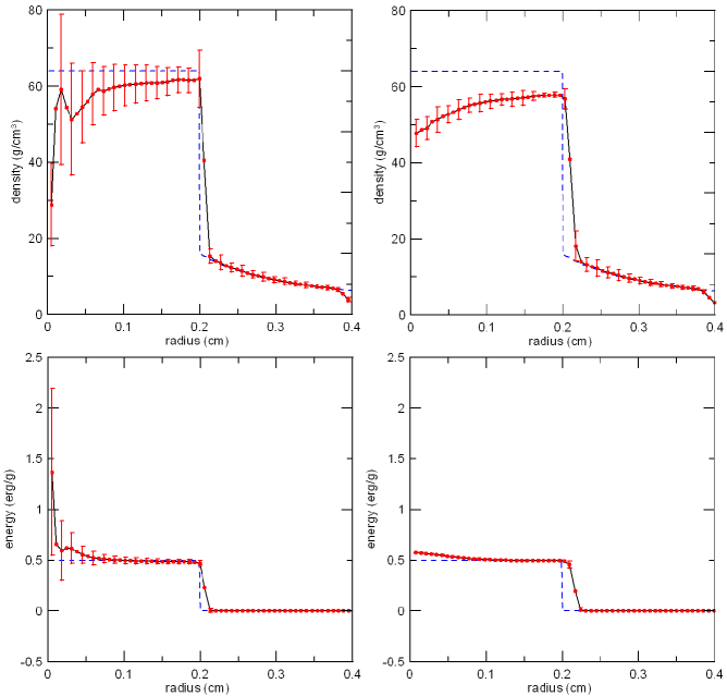
Figure 8: Results of the Noh test at t=0.6 s. Upper left and right: averaged density profiles without and with the artificial heat conduction. Bottom left and right: same but for internal energy. Dispersion around the averaged values are given by the error bars.

4.5 Supersonic collision of two streams of gas

Our last test is specifically addressed to check momentum conservation in a very anisotropic situation: the supersonic collision along the Z-axis of two homogeneous spherical clouds of gas with different size and mass. The size and mass of the spheres are $R_{1}=1$ cm; $M_{1}=4\pi/3$ g and $R_{2}=3$ cm; $M_{2}=36\pi$ g respectively so that their density is $\rho_{1}=\rho_{2}=1$ g.cm^-3. The biggest sphere is at rest with its center located at $(0,0)$ cm while the smaller one is centered at $(0,-5)$ cm moving upwards with velocity $v_{z}^{0}=10$ cm.s^-1. The initial internal energy of both spheres was $u_{1}^{0}=u_{2}^{0}=10^{-3}$ erg.g^-1 whereas EOS obeys an ideal gas law with $\gamma=5/3$. The corresponding initial Mach number was $M_{\mathrm{s}}^{0}\simeq 500$ thus the impact is supersonic. The number of particles in each sphere was $N_{1}=5480$ and $N_{2}=50334$ respectively.

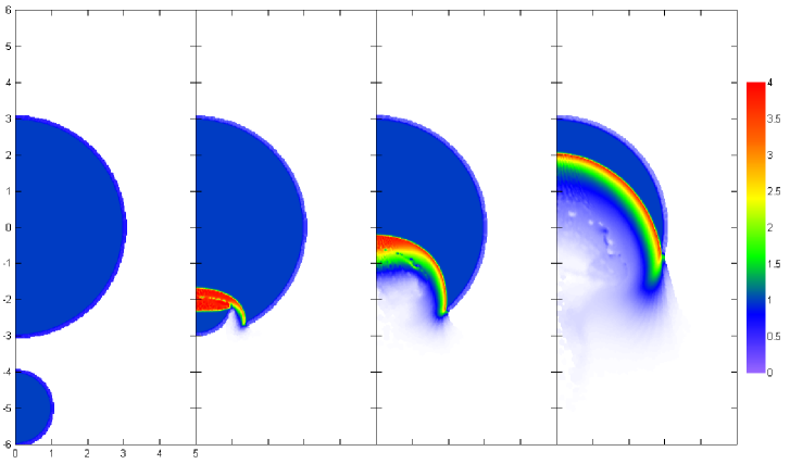
Figure 9: Density colour-map of the collision of two streams of gas at times t$=0$ s, t$=0.31$ s, t$=0.69$ s and t$=1.41$ s. Axis units are in centimeters.

In Fig. 9 there are represented several snapshots showing the density evolution during the collision process. As can be seen the large mass contrast leads to the complete deformation of the smaller sphere which, in the end transfers most of its initial momentum to the larger bubble. Information about the evolution of the center of mass of each bubble as well as that of the whole system is provided in Fig. 10. According to Figs. 9 and 10 the collision history can be roughly divided in three stages: 1) For $0\leq t\leq 0.5$ s, the incoming smaller cloud deforms while a large fraction of its kinetic energy went into internal energy around the collision region. A shock wave was launched into the larger bubble, 2) Between $0.5\leq t\leq 1$ s the total internal energy did not change so much. At $t=1$ s the velocity of the center of mass of both structures was practically the same, 3) For $t>1$ s the energy stored as internal energy is again restored to the system. At larger times the velocity of the smaller bubble became negative while the bigger cloud acquired a positive velocity to preserve total momentum. At our last time $t=1.4$ s the interaction between both structures is coming to an end. Fig. 10 also shows that, in spite of the large changes in the velocity of each bubble, the velocity of the center of mass of the whole system remained unaltered.

In the last row of Table 1 there are shown several magnitudes related to momentum and energy conservation. Conservation of linear momentum during the interaction was monitored through the displacement of the center of mass of the system. At the final time, $t=1.4$ s, the deviation of the center of mass position with respect the value expected from $\bar{v}_{z}^{0}t$ was much larger than that shown in the other tests. Still the relative error in the position of the center of mass once the collision has practically ceased was $\simeq 10^{-3}$. Angular momentum was very well preserved, almost to machine precision. Total energy was conserved to $10^{-2}$ relative to the initial kinetic energy of the system.

In an attempt to understand the origin of the discrepancy relative to momentum conservation in the Z-direction we ran exactly the same model but this time symmetrizing equation (13) (multiplying the term $P_{j}r_{j}/\hat{\eta}_{j}^{2}$  by $f_{1}^{j}$). There were no significant changes. We conclude that strict total momentum conservation in the Z-direction was not possible because of the interaction between real and reflected particles. Such interaction took place in a small band around the symmetry axis, acting as an external force which modified momentum of real particles. However that force can not be balanced by an opposite force acting in the left semiplane because, in the Z-direction, reflected particles were obliged to move exactly in the same way real particles did. Therefore if strong directional anisotropies appear in the vertical displacements of the mass points some degree of violation in momentum conservation is unavoidable. Eventually momentum conservation should improve as the number of particles increase because the amount of mass settled in the axis vicinity is lower.

Figure 10: Evolution of $\bar{v}_{z}$ of the center of mass of each bubble and of the system. Subscripts 1 and 2 refers to the smaller and larger bubble respectively. Evolution of total kinetic and internal energy is also given.

5 Conclusions

Despite the success of the smoothed particle hydrodynamics technique to handle gas-dynamics problems in three dimensions little effort has been invested to develop two-dimensional (axisymmetric) applications. This work intends to fill that gap by solving many of the problems often invoked in connection with SPH in cylindric coordinates. These are the treatment of the singularity axis, the handling of shock and thermal waves and, in many astrophysical scenarios, an accurate procedure to calculate the gravitational force. Our general philosophy in developing the mathematical formalism was to remain as close as possible to the cartesian scheme so that many of the results of the standard SPH in three dimensions can be extrapolated with minimum changes to the axisymmetric version.

Starting from the fluid Euler equations given by Brookshaw (2003) we have obtained analytical corrections to those particles which move close to the singularity axis. These corrections appear as multiplicative factors to the different terms of the fluid equations. Such multiplicative factors become equal to one when $r>2h$ (Fig. 1) so that there is no need to calculate them beyond that distance and the method is computationally efficient. Once the basic formalism was built we added several pieces of physics which make the scheme well suited to handle a large variety of problems. First of all an extension of the 3D standard artificial viscosity to the 2D-axisymmetric realm was devised, equations (23), (24) and (25). The artificial viscosity includes the convergence of the flow towards the symmetry axis via linear and quadratic terms proportional to $[\frac{v_{r}~{}h}{r}]$  (being r the distance to the symmetry axis). These terms arise because the diagonal part of the stress tensor in cylindric coordinates includes the divergence of the flow velocity. However the cartesian part of the divergence was already present in the standard formulation given by equations (22) and (23) giving rise to bulk and shear viscosity. Therefore only the axis converging part of velocity divergence, proportional to $v_{r}/r$ has been added. The resulting viscous force $\Pi^{2D}$  has two terms: $\Pi^{(1)}$ (cartesian) and $\Pi^{(2)}$ (axis converging part) which are calculated using similar expressions, equations (23), (25) involving four constants $\alpha_{0},\beta_{0}$ ($\Pi^{(1)}$) and $\alpha_{1},\beta_{1}$ ($\Pi^{(2)}$). The axis converging part of viscosity will be of importance only for strong implosions. Although in the simulations reported in this paper we have taken $\alpha_{0}=\alpha_{1}=1$ and $\beta_{0}=\beta_{1}=2$ there could be other plausible combinations worth to explore. A similar approach was used to built the conductive transport equation. Starting from the expression given by Brookshaw (1985) we have added a new term that accounts for the divergence of the temperature gradient in the axis neighborhoods. Even though the resulting expression was not totally antisymmetric it led to a satisfactory energy conservation in the tests described in sections 4.1 and 4.3. Finally the set of equations was completed with the inclusion of self-gravity. In axisymmetric geometry it is better to rely in the direct, ring to ring, interaction to compute gravity. Such procedure, although in general computationally expensive, has several advantages: 1) it does not rely in any sort of grid and gives the exact value of the gravitational force, 2) the calculations are feasible for a moderate number of particles (i.e. around $5~{}10^{4}$ in serial desktop machines) which often suffice in many 2D simulations 3) the scheme is clear and extremely simple making it straightforward to parallelize. The algorithm devised to compute gravity was able to keep track the free-fall collapse of an homogeneous sphere as well as of an homogeneous rotating cylinder. Given an initial amount of rotation the evolution of any point of the cylinder was handled by imposing angular momentum conservation around the symmetry axis.

Five test cases aimed at validating the computational scheme were considered. Each of them intended to check a particular physics item: heat conduction (Sects. 4.1 and 4.4), shock waves (Sect. 4.3 and 4.4) and gravity (Sects. 3.3.1 and 4.2). Momentum conservation was specially checked in Sect. 4.5. Because for the most part the initial configurations had spherical symmetry the preservation of that symmetry during the collapse and further expansion of the system was taken as an indicator of the general ability of the scheme to handle large changes in the spatial scale. It was also possible to make detailed comparisons of the results with those obtained either from analytical calculations, as in the case of the thermal wave propagation, or from one-dimensional simulations carried out using standard lagrangian hydrodynamics. The results, obtained using several dozen thousand particles, were in good agreement with the analytical expectations and to the 1D simulations. Additionally there was an almost perfect momentum conservation while numerical energy losses always remained lesser than $1\%$. The spherical symmetry was well preserved although a slight deviation was observed in the capsule implosion test, partially due to the so called hour-glass instability (owing to the initial setting of the particles in a lattice) and, despite the corrective terms, to the effect introduced by the singularity axis onto the approaching particles. A similar but probably more demanding test was the wall heating shock problem, dealing to the spherically symmetric implosion of a supersonic stream of gas. Although the results are not as good as those obtained with other methods which do not use artificial viscosity, they are comparable with one-dimensional calculations with similar resolution relying in artificial viscosity schemes. However the results improved when artificial heat conduction, calculated using equations (35) and (53), was switched-on.

As discussed in Sect. 4.5 a weak point of the formulation is that the inclusion of reflective particles in the scheme could degrade total momentum conservation in the Z-direction. However good momentum conservation, much better than energy conservation for instance, is expected in those systems in which the velocity field is not too anisotropic. If strong momentum exchange along the Z-axis is expected, as in the test described in Sect. 4.5, then momentum will be preserved to a similar level as total energy.

As a conclusion we can say that the formulation of the axisymmetric SPH given in this paper is a solid tool to carry out simulations using that particle method. However there are still a number of unresolved issues which deserve further development. One of them is how to build good initial models without settling particles of different mass in regular lattices. This is important because ordered lattices introduce spurious instabilities in the system and the mixing of particles with very different masses could lead to numerical artifacts. Another point of difficulty has to do with artificial viscosity, because it introduces too much shear viscosity in the system damping the natural development of hydrodynamical instabilities. The new term $\Pi_{ij}^{(2)}$ given by equation (25) of artificial viscosity comes from the diagonal of the stress tensor so its contribution to shear viscosity is probably lower than that of $\Pi_{ij}^{(1)}$. In any case the artificial viscosity formulation given in this work is so close to the standard formulation that it could benefit from future advances in the much better studied three-dimensional SPH. Finally, the simple test about the implosion of a rotating cylinder indicates that axisymmetric SPH is able to handle rotating structures but more work needs to be done to incorporate angular momentum transport into the numerical scheme.

5.1 Appendices

Appendix A Correction factors close to Z-axis

First, we derive the factor $f_{1}$ affecting the 2D-density $\eta$. Close to the Z-axis symmetry enforces the 3D-density $\rho$ to have a maximum or a minimum. Thus we can safely assume $\rho=\rho_{0}$ in the axis vicinity. If we make the one-dimensional SPH estimation of the averaged density along the r-axis:

$$<\eta(r)>=\int\limits_{-\infty}^{\infty}\eta(r^{\prime})W^{1D}(\frac{|r-r^{\prime}|}{h})dr^{\prime}$$ (61)

where $W^{1D}$ is the cubic-spline kernel in 1D:

$$W^{1D}(u_{r})=\frac{2}{3h}\cases{1-\frac{3}{2}u_{r}^{2}+\frac{3}{4}u_{r}^{3}\qquad\qquad 0\leq u_{r}\leq 1\cr\cr\frac{1}{4}(2-u_{r})^{3}\qquad\qquad\qquad 1<u_{r}\leq 2\cr\cr 0\qquad\qquad\qquad\qquad\qquad\quad u_{r}>2\cr}$$ (62)

being $u_{r}=|(r-r^{\prime})|/h$. If we take $\eta(r^{\prime})=2\pi|r^{\prime}|\rho_{0}$, which is only valid for $r^{\prime}\rightarrow 0$:

$$<\eta(r)>=2\pi\rho_{0}\int\limits_{-\infty}^{\infty}|r^{\prime}|W^{1D}(\frac{|r-r^{\prime}|}{h})dr^{\prime}$$ (63)

Using the cubic-spline the right side of equation (A3) can be integrated to give:

$$<\eta(r)>=\frac{\widehat{\eta}}{f_{1}(\zeta)}$$ (64)

where $\zeta=r/h$ and $\widehat{\eta}=2\pi r\rho$ is the corrected density (hereafter we put a hat over any corrected quantity). The correction factor $f_{1}(\zeta)$ is given by equation (5). The density in brackets is what SPH computes using summatories instead of integrals. Thus, adding the z-coordinate and using $W^{2D}$ the corrected density can be evaluated using:

$$\widehat{\eta}(r)=<\eta>f_{1}(\zeta)=\left(\sum_{j=1}^{N}m_{j}W^{2D}(|\mathbf{r_{i}-r_{j}|},h_{i})\right)\times f_{1}^{i}$$ (65)

A similar procedure can be used to get the adequate expressions for $\eta v_{r}$  and $\eta v_{z}$, needed to compute the temporal evolution of density, equation (15). Symmetry enforces the radial velocity to vanish at the symmetry axis, thus close to that axis $v_{r}=Cr$ and:

$$<\eta v_{r}>=\rho(z)2\pi K^{1D}C\int\limits_{-\infty}^{\infty}|r^{\prime}|r^{\prime}W_{r}(u_{r})dr^{\prime}$$ (66)

Again the integral on the right admits an analytical solution for the cubic-spline kernel. After a little algebra the following expression is obtained:

$$<\eta v_{r}>=\frac{\widehat{\eta v_{r}}}{f_{2}(\zeta)}$$ (67)

where $f_{2}(\zeta)$ is given by equation (16). The expression inside the brackets is what the numerical code calculates using summatories instead of integrals. Thus, the corrected $\widehat{\eta v_{r}}$, value of that magnitude is:

$$(\widehat{\eta v_{r}})_{i}=\left(\sum_{j=1}^{N}m_{j}v_{r_{j}}W(|\mathbf{s_{i}-s_{j}|},h_{i})\right)\times f_{2}^{i}$$ (68)

Similarly the correction to be applied to $\eta v_{z}$ is:

$$<\eta v_{z}>=\frac{\widehat{\eta v_{z}}}{f_{1}(\zeta)}$$ (69)

and its corresponding discrete expression is:

$$(\widehat{\eta v_{z}})_{i}=\left(\sum_{j=1}^{N}m_{j}v_{z_{j}}W(|\mathbf{s_{i}-s_{j}|},h_{i})\right)\times f_{1}^{i}$$ (70)

A plot of the factors $f_{1}(\zeta)$ and $f_{2}(\zeta)$ and their radial derivatives is given in Fig. 1. The factor $f_{1}(\zeta)$ is exactly one for $r=2h$ and goes to zero when $r/h\rightarrow 0$, as expected. However, it can be seen that factor $f_{2}(\eta)$ is close but not exactly one at $r=2h$ and its slope is not totally flat. This is because the integral expression in equation (A6) is quadratic in the radial coordinate $r$ thus the interpolation does not give the exact value of $<\eta v_{r}>$.

References

- Blondin et al. (1996) Blondin J.M., Lundqvist P., Chevalier R.A., 1996, ApJ, 472, 257
- Brookshaw (2003) Brookshaw L., 2003, ANZIAM J, 44, C114
- Brookshaw (1985) Brookshaw L., 1985, Proc. Astron. Soc. Aust., 6, 207
- Cabezón et al. (2008) Cabezón, R., García-Senz, D., Relaño, A., 2008, J. Comput. Phys.,227, 8523
- Gingold & Monaghan (1977) Gingold R.A., Monaghan J.J., 1977, MNRAS, 181, 375
- Herant & Benz (1992) Herant M., Benz W., 1992, ApJ, 387, 294
- Hernquist & Katz (1989) Hernquist L., Katz N., 1989, ApJS, 70, 419
- Jubelgas et al. (2004) Jubelgas M., Springel K., Dolag K., 2004 , MNRAS, 351, 423
- Lucy (1977) Lucy L.B., 1977, AJ, 82, 1013
- Monaghan (1989) Monaghan J.J., 1989, J. Comput. Phys.,82, 1
- Monaghan & Gingold (1983) Monaghan J.J., Gingold R.A., 1983, J. Comput. Phys.,52, 374
- Monaghan (1992) Monaghan J.J., 1992, ARAA, 30, 543
- (13) Monaghan J.J., 2005, Rep. Prog. Phys., 68, 1703
- Noh (1987) Noh W.F., 1987, J. Comput. Phys., 72, 78
- Omang et al. (2006) Omang, M., Borve S., Trulsen J., 2006, J. Comput. Phys., 213(1), 391
- Omang et al. (2007) Omang, M., Borve S., Trulsen J., 2007, Shock Waves, 16, 467
- Owen et al. (1998) Owen, J.M., Villumsen, J.V., Saphiro, P.R., Martel, H., 1998, ApJS, 116, 155
- Petscheck& Libersky (1993) Petscheck A.G., Libersky L.D., 1993, J. Comput. Phys., 109, 76
- Velarde et al. (2006) Velarde P., García-Senz D., Bravo E., Ogando P., Relaño A., García C., Oliva E., 2006, Physics of Plasmas, 13, 092901-1