Accuracy of bound-state form factors extracted from dispersive sum rules

Abstract

We discuss the extraction of form factors from three-point sum rules making use of harmonic-oscillator model, where we derive the exact expression for the relevant correlator. We determine the form factor of the ground state by the standard procedures adopted in the method of sum rules, and compare the obtained results with the known exact values. We show that the uncontrollable uncertainty in the extracted value of the form factor is typically much larger than that for the decay constant. In the example considered, we find the uncontrolled systematic error in the extracted form factor to exceed the 10% level.

1 Introduction

A QCD sum-rule calculation of hadron parameters svz ; ioffe involves two steps: (i) one calculates the operator product expansion (OPE) series for a relevant correlator and formulates the sum rule which relates this OPE to the sum over hadronic states, and (ii) one extracts the parameters of the ground state by some numerical procedure. Each of these steps leads to uncertainties in the final result.

The first step lies fully within QCD and allows for a rigorous treatment of the uncertainties: the correlator in QCD is not known precisely (because of uncertainties in quark masses, condensates, $\alpha_{s}$, radiative corrections, etc.) but the corresponding errors in the correlator may be controlled systematically (at least in principle).

The second step lies beyond QCD and is more cumbersome: even if several terms of the OPE for the correlator were known precisely, the hadronic parameters may be extracted from a sum rule only with limited accuracy – the corresponding error has to be treated as a systematic error of the employed method.

In this Letter, we continue our study of the systematic errors of hadron parameters obtained from dispersive sum rules. In an earlier analysis lms_sr we addressed the determination of the decay constant of the ground state by means of the two-point correlator. Here, we consider the extraction of the ground-state form factor from the three-point correlator in a quantum-mechanical harmonic-oscillator (HO) potential model. This simple model has strong advantages compared to more complicated cases: (i) it enables one to calculate the exact three-point function, and thus to generate the OPE to any order, and (ii) the bound-state parameters (masses, wave functions, form factors) are known precisely. Therefore, we may apply the standard sum-rule machinery to extract the form factor of the ground state and then compare it with the known exact form factor. In this way, we may probe the accuracy and reliability of the method. (For a discussion of many aspects of sum rules in quantum mechanics, we refer to nsvz ; nsvz1 ; qmsr ; orsay .)

We present an explicit example of the form factor extracted at a specific value of the momentum transfer, for which the exact correlator is described by the OPE with better than 1% accuracy and standard sum-rule techniques yield a form factor extremely stable in the Borel window. However, the value obtained from the sum-rule analysis differs from the exact value by more than 10%.

We therefore reinforce our previous statement that the standard procedures adopted in the method of sum rules do not allow one to obtain rigorous error estimates for the ground-state characteristics. In the case of form factors extracted from three-point correlators, the uncontrolled systematic errors may be considerably larger than those found in the case of decay constants extracted from two-point sum rules.

2 Harmonic-oscillator model

We consider a nonrelativistic model Hamiltonian $H$ with a HO interaction potential $V(r)$, $r\equiv|\vec{r}\,|$:

$$H=H_{0}+V(r),\qquad H_{0}={\vec{p}}^{\,2}/2m,\qquad V(r)={m\omega^{2}r^{2}}/{2}.$$ (2.1)

The full Green function $G(E)\equiv(H-E)^{-1}$ and the free Green function $G_{0}(E)\equiv(H_{0}-E)^{-1}$ are related by

$$G^{-1}(E)-G_{0}^{-1}(E)=V.$$ (2.2)

The solution $G(E)$ of this relation may be easily found by constructing its expansion in powers of the interaction $V$:

$$G(E)=G_{0}(E)-G_{0}(E)VG_{0}(E)+\cdots.$$ (2.3)

In our HO model, all characteristics of the bound states are easily calculable. For instance, for the ground state ($n=0$) one finds, with $q\equiv|\vec{q}|,$

$$E_{0}=\frac{3}{2}\omega,\qquad R_{0}\equiv|\Psi_{0}(\vec{r}=\vec{0})|^{2}=\left(\frac{m\omega}{\pi}\right)^{3/2},\qquad F_{0}(q)=\exp(-q^{2}/4m\omega),$$ (2.4)

where the elastic form factor of the ground state, $F_{0}(q),$ is defined according to

$$F_{0}(q)=\langle\Psi_{0}|J(\vec{q})|\Psi_{0}\rangle=\int d^{3}k\,\psi^{\dagger}(\vec{k})\psi(\vec{k}-\vec{q})=\int d^{3}r\,|\psi(\vec{r})|^{2}e^{i\vec{q}\vec{r}}$$ (2.5)

and the current operator $J(\vec{q})$ is given by the kernel

$$\langle\vec{r}\,^{\prime}|J(\vec{q})|\vec{r}\rangle=\exp(i\vec{q}\vec{r})\delta^{(3)}(\vec{r}-\vec{r}\,^{\prime}).$$ (2.6)

3 Polarization operator

The polarization operator

$$\Pi(T)=\langle\vec{r}_{f}=\vec{0}|\exp(-HT)|\vec{r}_{i}=\vec{0}\rangle$$ (3.7)

is used in the sum-rule approach for the extraction of the wave function at the origin (i.e., of the decay constant) of the ground state svz . A detailed analysis of the corresponding procedure for the HO model was presented in lms_sr . For the HO potential, the analytic expression for $\Pi(T)$ is known nsvz :

$$\Pi(T)=\left(\frac{\omega m}{\pi}\right)^{3/2}\frac{1}{\left[2\sinh(\omega T)\right]^{3/2}}.$$ (3.8)

The OPE series is the expansion of the exact quantity at small Euclidean time $T$ (or, equivalently, in powers of $\omega$):

$$\Pi_{\rm OPE}(T)=\left(\frac{m}{2\pi T}\right)^{3/2}\left(1-\frac{1}{4}\omega^{2}T^{2}+\frac{19}{480}{\omega^{4}T^{4}}+\cdots\right).$$ (3.9)

4 Vertex function

The basic quantity for the extraction of the form factor in the method of dispersive sum rules is the correlator of three currents ioffe . The analogue of this quantity in quantum mechanics is

$$\Gamma(E_{2},E_{1},q)=\langle\vec{r}_{f}=\vec{0}|(H-E_{2})^{-1}J(\vec{q})(H-E_{1})^{-1}|\vec{r}_{i}=\vec{0}\rangle,\qquad q\equiv|\vec{q}|,$$ (4.10)

[with the operator $J(\vec{q})$ defined in (2.6)] and its double Borel (Laplace) transform under $E_{1}\to\tau_{1}$ and $E_{2}\to\tau_{2}$

$$\Gamma(\tau_{2},\tau_{1},q)=\langle\vec{r}_{f}=\vec{0}|\exp(-H\tau_{2})J(\vec{q})\exp(-H\tau_{1})|\vec{r}_{i}=\vec{0}\rangle.$$ (4.11)

For large $\tau_{1}$ and $\tau_{2}$ the correlator is dominated by the ground state:

$$\Gamma(\tau_{2},\tau_{1},q)\to|\psi_{n=0}(r=0)|^{2}e^{-E_{0}(\tau_{1}+\tau_{2})}F_{0}(q^{2})+\cdots.$$ (4.12)

Let us notice the Ward identity which relates the vertex function at zero momentum to the polarization operator:

$$\Gamma(\tau_{1},\tau_{2},q=0)=\Pi(\tau_{1}+\tau_{2}).$$ (4.13)

This expression follows directly from the relation

$$J(\vec{q}=0)=1.$$ (4.14)

In HO model, we find the exact analytic expression for $\Gamma(\tau_{2},\tau_{1},q)$ by using the results for the Green function in configuration space $\langle\vec{r}\,^{\prime}=\vec{0}|G(T)|\vec{r}\rangle$ from nsvz . For our further investigation, we consider the vertex function for equal times $\tau_{1}=\tau_{2}=\frac{1}{2}T,$ which has the following explicit form:

$$\Gamma(T,q)=\left(\frac{m\omega}{\pi}\right)^{3/2}\frac{1}{\left[2\sinh(\omega T)\right]^{3/2}}\exp\left(-\frac{q^{2}}{4m\omega}\tanh\left(\frac{\omega T}{2}\right)\right).$$ (4.15)

The correlator is a function of two dimensionless variables $\omega T$ and $q^{2}/m\omega$.

Let us now construct for $\Gamma(T,q)$ the analogue of the OPE as used in the method of three-point sum rules in QCD. The corresponding procedure consists of two steps: First, we expand $\Gamma$ in powers of $\omega^{2}$ and obtain

$$\Gamma(T,q)=\sum\limits_{n=0}\Gamma_{2n}(q,T)\omega^{2n}.$$ (4.16)

Each term in this expansion can be computed from the diagrams depicted in Fig. 1.

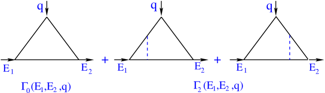
Fig. 1: Expansion of the correlator $\Gamma(E_{1},E_{2},q)$ in powers of the interaction.

This is, however, not the full story: In three-point sum rules one works with local condensates and, therefore, has for each $\Gamma_{2n}$, $n\geq 1,$ a power-series expansion in $T$. To keep the same track, we expand $\Gamma_{2n}$, $n\geq 1,$ in powers of $T$.

In applications, we keep the terms $\Gamma_{0},\ldots,\Gamma_{6}$ and omit higher-order terms; we then obtain the power corrections by expanding $\Gamma_{2}$, $\Gamma_{4}$, and $\Gamma_{6}$ in powers of $T$ retaining terms up to order $T^{8}$.

As the result of this procedure, the analogue of the OPE for $\Gamma$ takes the form

$$\Gamma_{\rm OPE}(T,q)=\Gamma_{0}(T,q)+\Gamma_{\rm power}(T,q),$$

$$\qquad\Gamma_{0}(T,q)=\left(\frac{m}{2\pi T}\right)^{3/2}\exp\left(-\frac{q^{2}T}{8m}\right),$$

$$\qquad\Gamma_{\rm power}(T,q)=\left(\frac{m}{2\pi T}\right)^{3/2}\left[-\frac{1}{4}\omega^{2}T^{2}+\frac{q^{2}\omega^{2}}{24m}T^{3}+\left(\frac{19}{480}\omega^{4}-\frac{5q^{4}\omega^{2}}{1536m^{2}}\right)T^{4}+\cdots\right].$$ (4.17)

We display here only terms up to $O(T^{4})$ in $\Gamma_{\rm power}$ but in calculations retain terms up to $O(T^{8})$ and $O(\omega^{6})$. These terms, as well as higher-order terms, may be easily generated from the exact expression (4.15).

It should be emphasized that the coefficients of each power of $T^{n}$ in the square brackets of (4) are polynomials in $q^{2}$ of order $(n-2)$. Therefore, if the momentum $q$ increases, one needs to include more and more power corrections in order to have a certain accuracy of the truncated OPE series for $\Gamma$. In QCD, this implies the necessity to know and include condensates of higher dimensions and restricts the applicability of three-point sum rules to the region of not too large $q^{2}$.

Figure 2 demonstrates the behaviour of the exact correlator and the truncated OPE series as described above for a fixed momentum transfer $q_{0}=1.5\,\omega$.

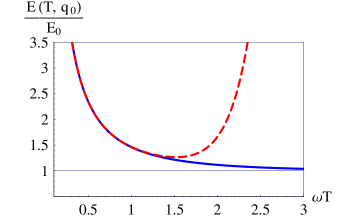
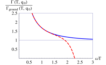
(a)	(b)
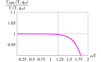
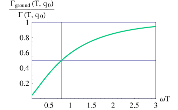
(c)	(d)

Fig. 2: (a) The energy $E(T,q_{0})=-\partial_{T}\log\Gamma(T,q_{0})$ and (b) the correlator $\Gamma(T,q_{0})$ for $q_{0}=1.5\,\omega$. Blue (full) line: calculation for the exact $\Gamma(T,q_{0})$; red (dashed) line: calculation for the truncated OPE series $\Gamma_{\rm OPE}(T,q_{0})$ with corrections up to order $(\omega T)^{8}$. (c) The accuracy of the truncated OPE for $\Gamma(T,q_{0})$ for $q_{0}=1.5\,\omega$. The vertical line at $q_{0}=1.2\,\omega$ is the upper boundary of the Borel window. (d) Relative contribution of the ground state to the correlator. The vertical line at $q_{0}=0.8\,\omega$ is the lower boundary of the Borel window.

Figures 2a,b make obvious how the ground-state form factor may be extracted from the correlator $\Gamma(T,q)$ known numerically (e.g., from the lattice): The correlator is dominated by the ground state at large values of $T$; so one may calculate the $T$- and $q$-dependent energy

$$E(T,q)=-\partial_{T}\log\Gamma(T,q),\qquad\partial_{T}\equiv\frac{\partial}{\partial T},$$ (4.18)

which exhibits a plateau at large $T$: $E(T,q)\to E_{0}$ for any $q$. Making sure that one has already reached the plateau and that the correlator is saturated by the ground state, one obtains the form factor from the relation

$$F_{0}(q)=\lim_{T\to\infty}\frac{1}{R_{0}}e^{E_{0}T}\Gamma(T,q).$$ (4.19)

Fig. 2c shows that the truncated OPE of (4) provides a good (say, better than 1% accuracy) description of $\Gamma(T,q)$ in the region $\omega T\leq 1.2$. The contribution of the excited states is still rather large in this region of $\omega T$ (see Fig. 2d) and thus a direct determination of the form factor from a truncated OPE is not possible. The procedures of the sum-rule method are aimed at modeling the contribution of higher states to the correlator and at obtaining in this way the ground-state form factor.

5 Sum rule

The sum rule is merely an expression of equality of the correlator calculated in the “quark” and in the hadron basis:

$$R_{0}e^{-{E_{0}}T}F_{0}(q)+\Gamma_{\rm excited}(T,q)=\Gamma_{0}+\Gamma_{\rm power}(T,q).$$ (5.20)

The quantity $\Gamma_{0}$ describes the free propagation and does not depend on the interaction. It may be written as a double spectral representation lms_prd75 :

$$\Gamma_{0}(T,q)=\int dz_{1}dz_{2}e^{-{\frac{1}{2}}z_{1}T}e^{-{\frac{1}{2}}z_{2}T}\Delta_{0}(z_{1},z_{2},q),\qquad\Delta_{0}(z_{1},z_{2},q)=\frac{1}{16\pi^{2}q}\theta\left((z_{1}+z_{2}-q^{2})^{2}-4z_{1}z_{2}<0\right).$$ (5.21)

Making use of the standard assumption that the contribution of the ground state is dual to the (rectangular) region of small values of $z_{1}$ and $z_{2}$, we obtain the relation:

$$R_{0}e^{-{E_{0}}T}F_{0}(q)=\int\limits_{0}^{z_{\rm eff}(T,q)}dz_{1}\int\limits_{0}^{z_{\rm eff}(T,q)}dz_{2}\,e^{-\frac{1}{2}z_{1}T}e^{-\frac{1}{2}z_{2}T}\Delta_{0}(z_{1},z_{2},q)+\Gamma_{\rm power}(T,q).$$ (5.22)

The above expression is exact if we use the exact $T$- and $q$-dependent effective continuum threshold, which cannot be calculated from the knowledge of only the OPE but can, of course, be reconstructed in our HO model, since we know the exact form factor (for details, see lms_sr ). Moreover, Eq. (5.22) may be even understood as the definition of the exact effective continuum threshold, if one makes use of the exact hadron parameters on the l.h.s. Therefore, this sum rule alone is not predictive. The form factor (as well as any other parameter) of the ground state may be obtained in the method of sum rules only if one imposes an independent criterion to fix the effective continuum threshold. It should be, however, understood that this procedure is essentially hand-made and does not arise from the underlying theory.

The standard assumption is to approximate $z_{\rm eff}(T,q)$ by a $T$-independent quantity, i.e., to replace it according to $z_{\rm eff}(T,q)\to z_{c}$. The quantity $z_{c}$ either may be chosen as a $q$-independent constant or may be adjusted for any value of $q$ separately.

We will now provide an example for the extraction of the form factor from sum rules where all the standard criteria point to a very accurate determination of the form factor; the actual error, however, turns out to be much larger.

Let us consider the extraction of the form factor at $q_{0}=1.5\,\omega$. This specific value is chosen on purpose: for this momentum transfer the sum rule for the form factor turns out to be most stable in the Borel window.

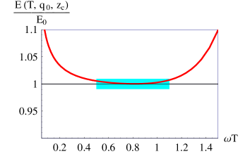
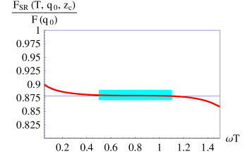
(a)	(b)
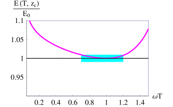
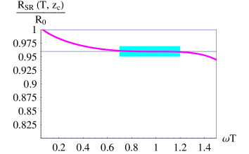
(c)	(d)

Fig. 3: (a) The energy of the cut correlator $E(T,q_{0},z_{c})=-\partial_{T}\log\Gamma(T,q_{0},z_{c})$ and (b) the sum-rule estimate for the form factor at $q_{0}=1.5\,\omega$ for $z_{c}=2.42\omega$. (c) The energy of the two-point cut correlator $E(T,z_{c})=-\partial_{T}\log\Pi(T,z_{c})$ and (d) the sum-rule estimate for the parameter $R_{0}$ for $z_{c}=2.454\omega$. The shaded rectangular areas indicate the regions of stability with 1% accuracy.

First, let us determine the “fiducial” interval (or “window”) of $T$ by the following two requirements: (i) The truncated OPE gives an approximation to the exact $\Gamma$ with, say, an accuracy better than 1%. This yields $\omega T\leq 1.2$. (ii) The ground state gives a sizeable contribution of, say, more than 50% to the correlator. This leads to $0.8\leq\omega T$. So the “window” where we will work to extract the ground-state form factor is $0.8\leq\omega T\leq 1.2$.

Next, we need to impose a criterion in order to fix $z_{c}$. A widely used procedure is the following jamin : One calculates

$$E(T,q_{0},z_{c})\equiv-\partial_{T}\log\Gamma(T,q_{0},z_{c}),$$ (5.23)

which depends on $T$ because of the approximation $z_{\rm eff}(T,q_{0})\to z_{c}$ (for details, consult lms_sr ). Then, one determines $z_{c}$ such that the function $E(T,q_{0},z_{c})$ has a horizontal tangent $E=E_{0}$, see Fig. 3a. This gives $z_{c}=2.42\omega$, which is used to calculate the form factor via Eq. (5.22) by the replacement $z_{\rm eff}(T,q_{0})\to z_{c}$. Our results are shown in Fig. 3b. The form factor is perfectly flat in the Borel window but nevertheless turns out to be by more than 10% lower than the known true value. For comparison, we present in Figs. 3c,d the corresponding plots for $R_{0}$ extracted from the sum rule for $\Pi(T)$ from lms_sr . Clearly, the general picture in both cases is similar but the deviation from the exact result is much greater for the form factor than for the decay constant.

Let us emphasize a rather dangerous point: (i) a perfect description of $\Gamma(T,q_{0})$ with better than 1% accuracy in the “window”, (ii) the deviation of $E(T,q_{0},z_{c})$ from $E_{0}$ at the level of only 1%, and (iii) a very good stability of $F(T,q)$ with better than 1% in the full “window” lead to an error of more than 10% in the extracted value of $F(q_{0})$! Clearly, this error could not be guessed on the basis of the other numbers obtained: the full picture mimics a very accurate extraction of the form factor, which is, however, certainly not the case.

6 Conclusions

Let us summarize the lessons one should learn from our analysis:

1. The knowledge of the correlator in a limited range of relatively small Euclidean times (that is, large Borel masses) is not sufficient for the determination of the ground-state parameters. As a consequence, a sum-rule extraction of the ground-state parameters without knowing the contribution of the hadronic continuum suffers from uncontrolled systematic uncertainties.

2. Modeling the hadron continuum by a Borel-parameter-independent effective continuum threshold $z_{c}$ allows one to fix this quantity $z_{c}$ by, e.g., requiring the average energy $E(T)$ to be close to $E_{0}$ in the Borel window. In this case, however, the error of the extracted ground-state parameter turns out to be typically much larger than

(i) the error of the description of the exact correlator by the truncated OPE and

(ii) the variation of the bound-state parameter in the Borel window.

3. It is important to realize that the Borel stability of the extracted ground-state parameter — the standard criterion that is believed to control both the reliability and the accuracy of the extracted ground-state parameter — does not in fact guarantee the extraction of its true value.

4. The adopted standard procedures for estimating the errors of the extracted bound-state parameters do not allow one to provide realistic error estimates.

The impossibility to control, at present, the systematic errors of the extracted hadron parameters is the weak feature of the sum-rule method and an obstacle for using the results from QCD sum rules for precision physics, such as electroweak physics.

Finally, we would like to comment on the obtained quantitative estimates. In HO model, the ground state is well separated from the first excitation, which contributes to the correlator, by a large gap of $2\omega$. This makes the HO model a very favourable case for the application of sum rules. Whether or not a comparable accuracy may be achieved in QCD, where this feature is absent, is questionable.

Acknowledgments: The authors are grateful to Hagop Sazdjian for interesting discussions. D. M. would like to thank the theory group of the Institut de Physique Nucléaire, Université Paris-Sud for hospitality during his stay in Orsay. D. M. gratefully acknowledges financial support from the Austrian Science Fund (FWF) under project P17692, RFBR under project 07-02-00551, and CNRS.

References

- (1) M. Shifman, A. Vainshtein, and V. Zakharov, Nucl. Phys. B 147 (1979) 385.
- (2) B. L. Ioffe and A. V. Smilga, Phys. Lett. B 114 (1982) 353; V. A. Nesterenko and A. V. Radyushkin, Phys. Lett. B 115 (1982) 410.
- (3) W. Lucha, D. Melikhov, and S. Simula, Phys. Rev. D 76 (2007) 036002; Phys. Lett. B 657 (2007) 148; Phys. Atom. Nucl. 71 (2008) 1461.
- (4) V. Novikov, M. Shifman, A. Vainshtein, and V. Zakharov, Nucl. Phys. B 237 (1984) 525.
- (5) A. I. Vainshtein, V. I. Zakharov, V. A. Novikov, and M. A. Shifman, Sov. J. Nucl. Phys. 32 (1980) 840.
- (6) V. A. Novikov et al., Phys. Rep. 41 (1978) 1; M. B. Voloshin, Nucl. Phys. B 154 (1979) 365; J. S. Bell and R. Bertlmann, Nucl. Phys. B 177 (1981) 218; Nucl. Phys. B 187 (1981) 285; V. A. Novikov, M. A. Shifman, A. I. Vainshtein, and V. I. Zakharov, Nucl. Phys. B 191 (1981) 301.
- (7) A. Le Yaouanc et al., Phys. Rev. D 62 (2000) 074007; Phys. Lett. B 488 (2000) 153; Phys. Lett. B 517 (2001) 135.
- (8) M. Jamin and B. Lange, Phys. Rev. D 65 (2002) 056005.
- (9) W. Lucha, D. Melikhov, and S. Simula, Phys. Rev. D 75 (2007) 096002.