Look-Ahead Benchmark Bias
in Portfolio Performance Evaluation

Abstract: Performance of investment managers are evaluated in comparison with benchmarks, such as financial indices. Due to the operational constraint that most professional databases do not track the change of constitution of benchmark portfolios, standard tests of performance suffer from the “look-ahead benchmark bias,” when they use the assets constituting the benchmarks of reference at the end of the testing period, rather than at the beginning of the period. Here, we report that the “look-ahead benchmark bias” can exhibit a surprisingly large amplitude for portfolios of common stocks (up to $8\%$ annum for the S&P500 taken as the benchmark) – while most studies have emphasized related survival biases in performance of mutual and hedge funds for which the biases can be expected to be even larger. We use the CRSP database from 1926 to 2006 and analyze the running top 500 US capitalizations to demonstrate that this bias can account for a gross overestimation of performance metrics such as the Sharpe ratio as well as an underestimation of risk, as measured for instance by peak-to-valley drawdowns. We demonstrate the presence of a significant bias in the estimation of the survival and look-ahead biases studied in the literature. A general methodology to test the properties of investment strategies is advanced in terms of random strategies with similar investment constraints.

JEL codes: G11 (Portfolio Choice; Investment Decisions), C52 (Model Evaluation and Selection)

Keywords: survival bias, look-ahead bias, portfolio optimization, benchmark, investment strategies

1 Introduction

Market professionals and financial economists alike strive to estimate the performance of mutual funds, of hedge-funds and more generally of any financial investment, and to quantify the return/risk characteristics of investment strategies. Having selected the funds and/or strategies of interest, a time-honored approach consists in quantifying their past performance over some time period. A large literature has followed this route, motivated by the eternal question of whether some managers/strategies systematically outperform others, with its implications for market efficiency and investment opportunities.

Backtesting investment performance may appear straightforward and natural at first sight. However, a significant literature has unearthed, studied and tried to correct for ex-post conditioning biases, which include the survival bias, the look-ahead bias and data-snooping, which continue to pollute even the most careful assessments. Here, we present a dramatic illustration of a variant of the look-ahead bias, that we refer to as the “look-ahead benchmark bias,” which surprised us by the large amplitude of the overestimation of expected returns of up to $8\%$ per annum. This overestimation is comparable to the largest amplitudes of the survival biases and look-ahead biases found for mutual funds or hedge-funds. We demonstrate the generic nature of the “look-ahead benchmark bias” by studying the performance of portfolios investing solely in regular stocks using very simple strategies, such as buy-and-hold, Markovitz optimization or random stock picking.

The look-ahead benchmark bias that we document is strongly related to the look-ahead bias proper and to the survival bias, but has no particular relation to data-snooping [Lo_etal90, White00, Sullivanetal99], which we therefore do not discuss further.

The standard survivorship bias refers to the fact that many estimates of persistence in investment performance are based on data sets that only contain funds that are in existence at the end of the sample period; see, e.g. [BrownGoetzmannIbbotsonRoss1992, GrinblattTitman92]. The corresponding survivorship bias is caused by the fact that poor performing funds are less likely to be observed in data sets that only contain the surviving funds, because the survival probabilities depend on past performance. Perhaps less appreciated is the fact that stocks themselves have also a large exit rate and hence also suffer from the survival bias. For instance, Knaup05 examines the business survival characteristics of all establishments that started in the United States in the late 1990s when the boom of much of that decade was not yet showing signs of weakness, and finds that, if 85% of firms survive more than one year, only 45% survive more than four years. Bartelsmanetal03 confirm that a large number of firms enter and exit most markets every year in a group of ten OECD countries: data covering the first part of the 1990s show the firm turnover rate (entry plus exit rates) to be between 15 and 20 per cent in the business sector of most countries, i.e. a fifth of firms are either recent entrants or will close down within the year. And this phenomenon of firm exits is not confined to small firms. Indeed, in the exhaustive CRSP database of about 26’900 listed US firms, covering the period from Jan. 1926 to Dec. 2006 (Center for Research in Security Prices, http://www.crsp.com/), we find that on average 25% of names disappeared after 3.3 years, 75% of names disappeared after 14 years and 95% of names disappeared after 34 years.

The standard look-ahead bias refers to the use of information in a simulation that would not be available during the time period being simulated, usually resulting in an upward shift of the results. An example is the false assumption that earnings data become available immediately at the end of a financial period. Another example is observed in performance persistence studies, in which it is common to form portfolios of funds/stocks based upon a ranking performed at the end of a first period, together with the implicit or explicit condition that the funds/stocks are still in the selected ranks at the end of the second testing period. In other words, funds/stocks that are considered for evaluation are those which survive a minimum period of time after a ranking period [BrownGoetzmannIbbotsonRoss1992]. This bias is not remedied even if a survivorship free data-base is used, because it reflects additional constraints on ranking.

More generally, the fact that a data set is survivorship free does not imply that standard methods of analysis do not suffer from ex-post conditioning biases, which in one way or another may use (often implicit or hidden) present information which would not have been available in a real-time situation.

Previous works have investigated both survivorship and look-ahead biases. BrownGoetzmannIbbotsonRoss1992 have shown that survivorship in mutual funds can introduce a bias strong enough to account for the strength of the evidence favoring return predictability previously reported. CarpenterLynch1999 find, among other results, that look-ahead biased methodologies (which require funds to survive a minimum period of time after a ranking period) materially bias statistics. ter Horst_etal01 introduce a weighting procedure based upon probit regressions which models how survival probabilities depend upon historical returns, fund age and aggregate economy-wide shocks, and which provides look-ahead bias-corrected estimates of mutual fund performances. Baquero_etal05 apply the methodology of ter Horst_etal01 to hedge-fund performance, which requires a well-specified model that explains survival of hedge funds and how it depends upon historical performance. ter Horst07 extend the look-ahead bias correction method of Baquero_etal05 to hedge-funds by correcting separately for additional self-selection biases that plague hedge-fund databases (underperformers do not wish to make their performance known while funds that performed well have less incentive to report to data vendors to attract potential investors).

The major part of the literature is devoted to assess the look-ahead bias on actively managed investment funds. Here, we are studying how the back-testing of investment strategies on biased stock price databases is effected. We add to the literature by focusing on the look-ahead bias that appears when the assets used to test the portfolio performance are selected on the basis of their relationship with the benchmark to which the performance is compared. In the next section 2, we provide a specific straightforward implementation using the S&P500 index as the benchmark over the period from January 2001 to December 2006. Section 3 is devoted to a more systematic illustration of the look-ahead benchmark bias over different periods, from 1926 to 2007. The substantial difference in the performances of up to 8$\%$ between portfolios with and without look-ahead bias provide an indication for the bias in the performance of the back-test of an active investment strategy as it is commonly carried out. Sections 2 and 3 document that passive strategies are higher in after cleaning the database with respect to the look-ahead bias. Under quite general assumptions, we give in Section 4 an analytical prediction for the look-ahead bias happening to the mean-variance investment rule which might be applied in a mutual fund. In particular, we discuss, under what conditions the naive diversification would be favorable. The same methodology can be applied to give decision support to the hedge fund manager whether she should equally allocate money to different alternative investment strategies. Section 5 extends on the empirical evidence presented in sections 2 and 3 by using random strategies. Random strategies are proposed as a simple and efficient test of the value added by a given strategy, which take into account all possible biases, including those too difficult to address or that are even unknown to the analyst.

2 A first recent illustration over the period from January 2001 to December 2006 using the S&P500 as the benchmark

Let us consider a manager who wants to back-test a given trading strategy on past data, namely on a pool of stocks such as the constituents of the S&P500 index on a given period, say January 2001 to December 2006. To do so, the natural approach would be the following:

1. Obtain the list of constituents of the S&P500 index at the present time (end of December 2006);

2. For each name (stock), retrieve the closing price time series for the given period from January 2001 to December 2006;

3. Backtest the strategy on that data set, for instance by comparing it with the S&P500 benchmark.

However, doing so introduces a formidable bias, and can easily lead to erroneous conclusions. Figure 1 dramatically illustrates the effect by comparing the performance of two investments.

In the first investment, which is subject to the look-ahead bias, we build $1 of an equally weighted portfolio invested in the 500 stocks constituting the S&P500 index at the end of the period (29 December 2006), and hold it from 1st January 2001 until 29th December 2006. Meanwhile, the second investment simply consists in buying $1 of an equally weighted portfolio invested in the 500 stocks constituting the S&P500 index at the beginning of the period (1st January 2001), and in holding it from 1st January 2001 until 29th December 2006. Both investments are buy-and-hold strategies and should have yielded similar performances if the constitution of the S&P500 index had not changed over this period. However, the list of constituents of the S&P500 index is updated, usually on a monthly basis, in order to include only the largest capitalizations of the US stock market at the current time. Consequently, this list of constituents cannot, almost per force, contain a stock that for instance crashed in the recent past. Indeed, in such a case, the stock has a large probability to be passed in terms of capitalization by another stock of the same industry branch and thus leave the index and be replaced by that other stock. The only difference in the two portfolios is that the first investment uses a look-ahead information, namely it knows on 1st January 2001 what will be the list of constituents of the S&P500 index at the end of the period (29th December 2006). This apparently innocuous look-ahead bias leads to a huge difference in performance, as can be seen in Figure 1 and from simple statistics: the first (respectively second) investment has an annual average compounded return of $6.4\%$ (resp. $2.3\%$) and a Sharpe ratio (non-adjusted for risk-free rate) of $0.4$ (resp. $0.1$). The first investment has significant better return but, what is even more important, it exhibits larger risk-adjusted returns.

For reference, we also plot the historical value of the actual S&P500 index, normalised to $1$ on 1st January 2001. Note that its performance is slightly worse than that of the second investment discussed above. This could be due to the different weighting and also to the effect reported by Cai_Houge07.

Many managers would have been happier to report Sharpe ratios in the range obtained for the first investment, especially over this turbulent time period. Investment strategies exhibiting this kind of performance would fuel interpretations that this is evidence of a departure from the efficient market hypothesis and/or of the existence of arbitrage opportunities. On the other hand, other pundits would observe that this look-ahead bias is really obvious, so that no one would fall into such a trivial trap. This quite reasonable assessment actually collides with one simple but often overlooked operational limitation of back-tests: the change of constitution of financial indices are not recorded in most standard professional databases, such as Bloomberg, Reuters, Datastream or Yahoo! Finance. As the standard goal for investment managers is at least to emulate or better to beat some index of reference, back-tests on comparative investments should use a defined set of assets on which to invest, which is defined at the beginning of the period. However, because the list of constituents of the indices is unexpectedly challenging to retrieve, it is common practice to use the set of assets constituting the benchmarks of reference at the present time, rather than at the beginning of the period. Then, necessarily, the kind of look-ahead bias that we report here will automatically pollute the conclusions, with sometimes dramatic consequences, as illustrated in Figure 1. We refer to this as the “look-ahead benchmark bias.”

A part of the over-performance of the ex-post portfolio over the S&P500 index can be attributed to the fact that the former is equally-weighted while the later is value-weighted. But this does not explain away the look-ahead effect as shown by the large difference between the equally-weighted ex-post and ex-ante portfolios. For instance, consider the DJIA. While the mean return of the price-weighted DJIA index from January 2001 to September 2007 was on slightly below ($3.2\%$ p.a) that of the price-weighted ex-post portfolio ($3.8\%$ p.a.), the difference is much larger for the period from February 1973 to September 2007: $5.7\%$ p.a. versus $7.8\%$ p.a.

3 The extent of the Look-Ahead Benchmark Bias

We use the data provided by the CRSP database, from which we extract the close price (daily), split factor (daily) and number of outstanding shares (monthly) for all US stocks from January 1926 to December 2006. This represents a total of 26’892 different stocks.

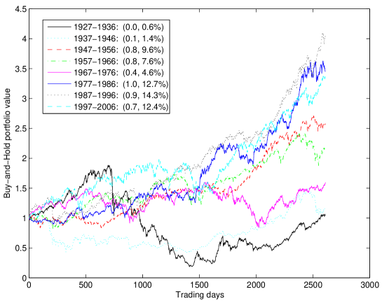
(a) biased, ex-post pickup

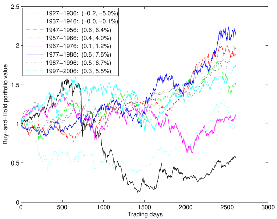
(b) ex-ante pickup

Figure 2: For each epoch of $10$ years, we plot the evolution of portfolio $1$ (upper panel) which invests $1 equally weighted on the $500$ largest stock capitalizations, as determined at the end of the ten-year period and the evolution of portfolio $2$ (lower panel) which invests $1 equally weighted on the $500$ largest stock capitalizations, as determined at the start of the ten-year period. Note the different ranges of the vertical scales in the two panels. The inserts give the Sharpe ratio (with zero risk-free rate) and continuously-compounded average annual return. The discrepancy between these two figures helps us visualise the extent of the survival bias for the $500$ largest capitalizations throughout time.

We decompose the time interval from January 1926 to December 2006 into $8$ periods of $10$ years each. For each period, we monitor the value of two portfolios. At the beginning of each ten-year period, the first ex-post (resp. second ex-ante) portfolio invests $1 equally weighted on the $500$ largest stock capitalizations, as determined at the end (resp. start) of the ten-year period. The first ex-post portfolio has by definition the look-ahead benchmark bias, while the second ex-ante portfolio is exempt from it and could have been implemented in real time. Figure 2 plots the time evolution of the value of the two portfolios. The inserted panels show that the Sharpe ratio and continuously-compounded average annual returns are much larger for portfolio $1$ compared with portfolio $2$.

Figure 3 shows the time evolution of the value of an investment consisting of being long $1 in the portfolio $1$ (ex-post) and short $1 in portfolio $2$ (ex-ante). In other words, it shows the ratio of the value of the ex-post portfolio $1$ divided by the value of the ex-ante portfolio $2$, for each of the $8$ periods. By construction, this hedged long-short portfolio can be implemented only ex-post when backtesting, and not in real-time. Its performance is consistently good over the $8$ periods from 1926 to 2006, with a huge reduction of risks and better returns than the unbiased, ex-ante portfolio $2$, thus demonstrating the significance of the look-ahead bias. This result is robust with respect to the number of stocks selected in the two portfolios.

Table 1 tests for different means in the ex-ante and ex-post portfolios. In the first two decades the means cannot be distinguished while in the recent decades the means differ significantly.

4 Theoretical estimation of the bias in estimations of the look-ahead and survival biases

We now show how one can analytically determine the estimation bias with regard to the true value of the bias, using the fact that the sample mean of an (equally weighted or Markowitz) portfolio of assets with normally distributed returns has a Wishart distribution. We find in particular that the level of the entries in the covariance matrix of the asset returns has an impact on the amount of the bias. This is relevant because a database with survival bias has a covariance matrix with smaller covariance terms, which tends to enhance the difference between the true and the biased dataset. These calculations can also be used for the survival bias, as discussed at the end of the section.

In the following, we calculate analytically the estimation error of the Sharpe Ratio based on data with bias versus the Sharpe Ratio based on data without bias. The derived expression depends on the true expected returns and covariance matrices of both data sets. Let us consider an economy characterized by a vector process of $N$ asset excess returns $\{R_{t},t=1,...,T\}$, which are normally distributed. Let $\mu$ be the vector of mean excess return, $\Sigma$ the covariance matrix of the excess returns and $\omega$ the vector of portfolio weights.

Markowitz’ optimization program consists in finding $\omega$ maximizing the following risk-adjusted excess return

$$U(\omega)=\omega^{\prime}\mu-{\gamma\over 2}\omega^{\prime}\Sigma\omega~{},$$ (1)

where $\gamma$ is the risk aversion coefficient. The optimal weights are

$$\omega^{*}={1\over\gamma}\Sigma^{-1}\mu~{},$$ (2)

with

$$U(\omega^{*})={1\over 2\gamma}\omega^{\prime}\Sigma^{-1}\omega={1\over 2\gamma}S_{*}^{2}~{},$$ (3)

where $S_{*}$ is the Sharpe ratio given by

$$S_{*}^{2}=\omega^{\prime}\Sigma^{-1}\omega~{}.$$ (4)

In contrast, the naive (equally weighted) diversification $\omega_{\rm EW}=c{\bf 1}_{N}$, where $c\in{\cal R}$ gives the following risk-adjusted excess return

$$U(\omega_{\rm EW})={1\over 2\gamma}S_{\rm EW}^{2}~{},$$ (5)

where the Sharpe ratio $S_{\rm EW}$ of the equally weighted portfolio is given by

$$S_{\rm EW}={({\bf 1}^{\prime}\mu)^{2}\over{\bf 1}_{N}^{\prime}\Sigma{\bf 1}_{N}}~{}.$$ (6)

Sample estimations of the mean excess return, covariance matrix and optimal Markowitz’ weights are

$${\hat{\mu}}={1\over T}\Sigma_{t=1}^{T}R_{t}~{},~{}~{}~{}{\hat{\Sigma}}={1\over T}\Sigma_{t=1}^{T}(R_{t}-{\hat{\mu}})(R_{t}-{\hat{\mu}})^{\prime}~{},~{}~{}~{}{\hat{\omega}}={1\over\gamma}{\hat{\Sigma}}^{-1}{\hat{\mu}}~{}.$$ (7)

Then, the sample excess returns ${\hat{\mu}}$ are distributed according to a multivariate normal distribution,

$${\hat{\mu}}\sim{\cal N}\left(\mu,{\Sigma\over T}\right)~{},$$ (8)

and the sample covariance matrix is distributed according to

$$T{\hat{\Sigma}}\sim{\cal W}_{N}\left(\Sigma,T-1\right)~{},$$ (9)

where ${\cal W}_{N}$ is the Wishart distribution.

Let the index “1” refer as in the above empirical tests to data with the look-ahead bias, and the index “2” to data without the bias. The true bias is $U(\omega_{1}^{*})-U(\omega_{2}^{*})$, while one only has access to the estimated bias $U({\hat{\omega}}_{1})-U({\hat{\omega}}_{2})$. To access how much the bias can be under- or over-estimated, the relevant measure is

$$\Delta\equiv\left[U(\omega_{1}^{*})-U(\omega_{2}^{*})\right]-\left[U({\hat{\omega}}_{1})-U({\hat{\omega}}_{2})\right]~{},$$ (10)

which can be expressed explicitly as

$$\Delta={1\over\gamma}(1-k)\left[S_{*,1}^{2}-S_{*,2}^{2}\right]={1\over\gamma}(1-k)\left(\omega_{1}^{\prime}\Sigma_{1}^{-1}\omega_{1}-\omega_{2}^{\prime}\Sigma_{2}^{-1}\omega_{2}\right]~{},$$ (11)

where

$$k={T\over T-N-2}\left(2-{T(T-2)\over(T-N-1)(T-N-4)}\right)<1~{}.$$ (12)

Suppose that the biased data is such that ${\bf 1}^{\prime}\mu_{1}>{\bf 1}^{\prime}\mu_{2}$ and ${\bf 1}_{N}^{\prime}\Sigma_{1}{\bf 1}_{N}<{\bf 1}_{N}^{\prime}\Sigma_{2}{\bf 1}_{N}$, which is indeed usually the case as reported above (large returns and smaller risks for the look-ahead biased data). Then, $\Delta>0$, i.e., the true bias is larger than estimated from the data. If the sample size $T$ is not too large compared with the number $N$ of assets, then the effect of the bias on the Sharpe Ratio is generally underestimated. This under-estimation is also found for the equi-weighted portfolio but its magnitude is larger for the Markowitz rule.

Other effects occur. For instance, consider portfolios made of a few tens of assets with the same expected returns and same variances, and with zero covariances. Then, the expected Sharpe ratio is slightly better for naïve diversification as compared to the sample-based Markowitz-optimal portfolio. Now, assume you have measured the expected returns and their covariance matrix based on data with the survival bias, where the mean and variances are higher than in bias-free data. Then, the expected measure of the Sharpe ratio gets higher for the sample-based Markowitz-optimal portfolio compared to the na ve diversification, that is, the order flips over. In the literature on the survival bias, the methodology is often to compare the performance measures estimated by sample versions of expected returns and their covariance matrix based on both a clean and a biased data base. As our calculations above show (and which apply straightforwardly also the survival bias), the assessment of the impact of the survivorship bias on the performance figures is biased itself. Under mild assumptions, one can conclude that the bias is worse than one thinks it is when reading the literature, which includes e.g. [BrownGoetzmannIbbotsonRoss1992, Brownetal95, Brownetal97, Brownetal99, Carhartetal02, CarpenterLynch1999, Eltonetal96].

5 Constrained Random Portfolios and proposed testing methodology

5.1 Robustness of the look-ahead benchmark bias using random strategies

Let us come back to the period from 1st January 2001 to 29th December 2006, shown in Figure 1 in order to test further the amplitude and robustness of the impact of the look-ahead benchmark bias. Investing on the 500 constituents of the S&P500 index at the end of the testing period (29th December 2006) amounts to bias the stock selection towards good performers. We illustrate that, as a consequence, non-informative random strategies exhibit very good to extremely good performance. We generate 10 portfolios, each of them implementing a random strategy. A random strategy opens only long positions (we buy first, and sell later) on a subset of the 500 stocks, with an average leverage of $0.8$ and an average duration per deal of $9$ days – which are common values. Given these constraints, the choice of the selected stock and the timing are random at each time step. We do not specify further the algorithm as all possible specific implementations give similar results.

Figure 4 plots the time evolution of the value of $1 invested in each of these ten random portfolios on 1st January 2001. These random portfolios provide an average compounded annual return of $(9.1\pm 4)\%$ with an excellent Sharpe ratio (with zero risk-free interest) of $2\pm 0.8$. The random portfolios (solid green lines) strongly outperform the S&P500 index (red dashed line), and simply diffuse around the look-ahead index (black dots) with an upward asymmetry. Similar results are obtained with other parameters of the random strategies.

5.2 Using random strategies on the same biased data as a general testing procedure

Because in practice one may never be in a position to completely exclude the presence of a look-ahead bias, we propose the use of constrained random portfolios on the same database as benchmarks against which to test the value of proposed investment strategies, so as to to assess the probability that the performance of a given strategy can be attributed to chance. Because the same look-ahead biases will impact both the random portfolios and the proposed strategies, one should thus be able to detect the presence of anomalously large gains that could result from a large amplitude of the look-ahead bias and quantify the real value, if any, of the proposed strategy over the random portfolios. This added value can be used as a useful metric of the performance of the proposed strategy. In order for this methodology to work, the constrained random portfolios should imitate as closely as possible the properties of the trading strategy about to be tested, such as its leverage, mean invested time and the turn-over.

6 Concluding remarks

We have reported a surprisingly large “look-ahead benchmark bias”, which results from an information on the future ranking of stocks due to their belonging to a benchmark index at the end of the testing period. We have argued that this look-ahead benchmark bias is probably often present due to (i) the need for strategies or investments to prove themselves against benchmark indices and (ii) the non-availability of the changes of composition of benchmark indices over the testing period. More generally, it is difficult if not impossible to completely exclude any look-ahead bias in simulations of the performance of investment strategies. As we reviewed in the introduction, one way to address these biases requires to first recognize their existence, and then to model how survival probabilities depend on historical returns, fund age and aggregate economy-wide shocks.

But, one can never be 100% certain that all biases have been removed. In certain scientific fields concerned with forecasting, such as in earthquake prediction for instance, the community has recently evolved to the recognition that only real-time procedures can avoid such biases and test the validity of models [Jordan06, Schorlemmer07]. Actually, real-time testing is a standard of the financial industry, since cautious investors only invest in funds that have developed a proven track record established over several years. But as shown in the academic literature, success does not equate to skill and may not be predictive of future performance, as luck and survival bias can also loom large [Barrasetal07]. There is a large and growing literature on how to test for data snooping and fund performance (see for instance [Lo_etal90, Romano_Wolf05, Wolf06]). The problem is more generally related to the larger issue of validating models (e.g., [Sornette_etal07] and references therein).

Practitioners should be careful to test for the presence of such a look-ahead bias in their dataset prior to backtesting their trading strategy. We have proposed a simple and practical way to do so, which consists in using random strategies, having as much of the characteristics of the strategy to be tested as is possible.

Table 1: Two-sample-t-test for indentical means (with unknown but common standard deviation) for the ex-post and ex-ante portfolios 1 and 2. The test uses the real one year interest rates as reported by R. Shiller.

Sub-sample	Test statistic	Significance level
1927-1936	0.7201	0.4807
1937-1946	0.3708	0.7151
1947-1956	1.4125	0.1749
1957-1966	1.9151	0.0715
1967-1976	3.2103	0.0049
1977-1986	2.3461	0.0306
1987-1996	2.6059	0.0179
1997-2006	1.9879	0.0622

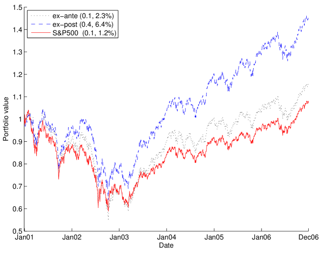
Figure 1: Evolution, from January 2001 to December 2006, of $1 invested in two equally weighted buy-and-hold portfolios made of the $500$ constituents of the S&P500 index, respectively as in 1st January 2001 (ex-ante portfolio) and 29th December 2006 (ex-post portfolio). For reference, we also plot the historical value of the actual S&P500 index, normalised to $1$ on 1st January 2001. The performance of these three portfolios are reported in the upper left panel, with their annualized Sharpe ratios (using a zero risk-free interest rate) and their continuously compounded average annual returns.

Figure 3: Time evolution of the value of an investment consisting in being long $1 in a portfolio $1$ equally weighted on the 500 largest stock capitalizations at the end of each period and short $1 in a portfolio $2$ equally weighted on the 500 largest stock capitalization at the end of each period, with compounding the returns. The inset shows the Sharpe ratios (with zero risk-free interest) and compounded annual return for the $8$ periods.

Figure 4: Time evolution of the value of $1 invested in each of five random portfolios (as described in the text) on 1st January 2001. The random portfolios (solid green lines) strongly outperform the S&P500 index (red dashed line), and simply diffuse around the look-ahead index (black dots) with an upward asymmetry.

References

- [1] \harvarditemBaquero et al.2005Baquero_etal05 Baquero, G., J. ter Horst and M. Verbeek (2005) Survival, look-ahead bias, and the persistence in hedge fund performance, Journal of Financial and Quantitative Analysis 40 (3), 493-517.
- [2] \harvarditemBarras et al.2007Barrasetal07 Barras, L., O. Scaillet and R. Wermers, False Discoveries in Mutual Fund Performance: Measuring Luck in Estimated Alphas, working paper (March 2007)
- [3] \harvarditemBartelsman et al.2003Bartelsmanetal03 Bartelsman, E., Scarpetta, S., Schivardi, F. (2003) Comparative Analysis of Firm Demographics and Survival: Micro-level Evidence for the OECD Countries, OECD Economics Department Working Papers, No. 348, OECD Publishing, doi:10.1787/010021066480.
- [4] \harvarditemBrown et al.1992BrownGoetzmannIbbotsonRoss1992 Brown, S.J., W. Goetzmann, R. G. Ibbotson and S. A. Ross (1992) Survivorship bias in performance studies, Review of Financial Studies 5 (4), 553-580.
- [5] \harvarditemBrown et al.1995Brownetal95 Brown, S.J., W.N. Goetzmann and S.A. Ross (1995) Journal of Finance 50, 853-873.
- [6] \harvarditemBrown et al.1997Brownetal97 Brown, S.J., W.N. Goetzmann, R.G. Ibbotson and S.A. Ross (1997) Rejoinder: The J-Shape Of Performance Persistence Given Survivorship Bias, Review of Economic Statistics 79, 167-170.
- [7] \harvarditemBrown et al.1999Brownetal99 Brown, S.J., W.N. Goetzmann and R.G. Ibbotson (1999) Offshore Hedge Funds: Survival and Performance, 1989-95, Journal of Business 72, 91-117.
- [8] \harvarditemCai and Houge2007Cai_Houge07 Cai, J. and T. Houge (2007) Index Rebalancing and Long-Term Portfolio Performance, Available at SSRN: http://ssrn.com/abstract=970839
- [9] \harvarditemCarhart et al.2002Carhartetal02 Carhart, M.M., J.N. Carpenter, A.W. Lynch and D.K. Musto, Mutual fund survivorship, Review of Financial Studies 15, 1439-1463.
- [10] \harvarditemCarpenter and Lynch1999CarpenterLynch1999 Carpenter, J.N. and A. W. Lynch (1999) Survivorship bias and attrition effects in measures of performance persistence, Journal of Financial Economics 54 (3), 337-374.
- [11] \harvarditemElton et al.1996Eltonetal96 Elton, E., M. Gruber, and C. Blake (1996) Survivorship Bias and Mutual. Fund Performance, Review of Financial Studies 9, 1097-1120.
- [12] \harvarditemGrinblatt and Titman1992 GrinblattTitman92 Grinblatt, M. and S. Titman (1992) The persistence of mutual fund performance, Journal of Finance 47, 1977-1984.
- [13] \harvarditemJordan2006Jordan06 Jordan, T. H. (2006) Earthquake Predictabillity: Brick by Brick, Seismological Research Letters 77 (1), 3-6.
- [14] \harvarditemKnaup2005Knaup05 Knaup, A.E. (2005) Survival and longevity in the Business Employment Dynamics data, Monthly Labor Review, May 2005, 50-56.
- [15] \harvarditemLo and McKinlay1990Lo_etal90 Lo, A.W. and A.C. McKinlay (1990) Data-snooping biases in tests of financial asset pricing models, Review of Financial Studies 3 (3), 431-467.
- [16] \harvarditemRomano and Wolf2005Romano_Wolf05 Romano, J.P. and M. Wolf (2005) Stepwise multiple testing as formalized data snooping, Econometrica 73 (4), 1237-1282.
- [17] \harvarditemSchorlemmer et al.2007Schorlemmer07 Schorlemmer, D., M. Gerstenberger, S. Wiemer, D.D. Jackson and D.A. Rhoades (2007) Earthquake Likelihood Model Testing, in Special Issue on Working Group on Regional Earthquake Likelihood Models (RELM), Seismological Research Letters 78 (1), 17.
- [18] \harvarditemSornette et al.2007Sornette_etal07 Sornette, D., A. B. Davis, K. Ide, K. R. Vixie, V. Pisarenko, and J. R. Kamm (2007) Algorithm for Model Validation: Theory and Applications, Proc. Nat. Acad. Sci. USA 104 (16), 6562-6567.
- [19] \harvarditemSullivan et al.1999 Sullivanetal99 Sullivan, R., A. Timmermann and H. White (1999) Data-Snooping, Technical Trading Rule Performance, and the Bootstrap, The Journal of Finance 54, 1647-1691.
- [20] \harvarditemter Horst et al.2001 ter Horst_etal01 ter Horst, J.R., T.E. Nijman and M. Verbeek (2001) Eliminating look-ahead bias in evaluating persistence in mutual fund performance, Journal of Empirical Finance 8, 345-373.
- [21] \harvarditemter Horst and Verbeek2007 ter Horst07 ter Horst, J. R. and M. Verbeek (2007) Fund Liquidation, Self-Selection and Look-Ahead Bias in the Hedge Fund Industry, Review of Finance, 1-28, doi:10.1093/rof/rfm012.
- [22] \harvarditemWhite2000 White00 White, H. (2000) A Reality Check for Data Snooping, Econometrica 68, 1097-1126.
- [23] \harvarditemWolf2006Wolf06 Wolf, M. (2006) The Skill of Separating Skill from Luck, working paper Univ. Zurich (August).
- [24]