Theoretical and numerical investigations on shapes of planar lipid monolayer domains

Abstract

Shapes of planar lipid monolayer domains at the air-water interface are theoretically and numerically investigated by minimizing the formation energy of the domains which consist of the surface energy, line tension energy, and dipole electrostatic energy. The shape equation which describes boundary curves of the domains at equilibrium state is derived from the first order variation of the formation energy. A relaxation method is proposed to find the numerical solutions of the shape equation. The theoretical and numerical results are in good agreement with previous experimental observation. Some new shapes not observed in previous experiments are also obtained, which awaits experimental confirmation in the future.

I INTRODUCTION

In the last three decades lipid monolayer domains (LMDs) at an air-water interface have drawn much attention from biochemists and physicists. Experimental researchers have observed that the lipid monolayer domains display many kinds of shapes, such as circular form, S form, dumbbell form, serpentine formA:Stine ; A:K.Y.C.Lee ; A:M.M.Lipp , torus formA:R.M.Weis85 ; A:H.M.McConnell90 , fan form, multi-leaves form with spiral armsA:K.Y.C.Lee ; A:M.M.Lipp ; A:R.M.Weis85 ; A:R.M.Weis84 ; A:H.E.Gaub ; A:Peter Kruger99 ; A:Peter Kruger (also called labyrinthine form) and so on, which brings a theoretical question: How to understand these shapes? McConnell et al. proposed that the shape of LMDs was a natural result of competition between the energy due to the line tension of domain boundary and the dipole electrostatic energy of lipid moleculesA:H.M.McConnell88 ; A:H.M.McConnell . By assuming that all lipid molecules align along the normal direction of the domain plane, they also proved that the total dipole electrostatic energy can be simplified as a double curve integral form along the domain boundary which will be called as McConnell energy in the following contents. Following McConnell’s seminal work, Iwamoto and Ou-Yang proposed that besides the above two kinds of energy, the growth of a lipid domain should cost an additional surface energy due to the difference in the Gibbs free energy density between outer (liquid-like disorder) and inner (solid-like order) phasesA:M.Iwamoto04 . Each observed LMD should minimize its “ formation energy ” (i.e., the sum of these three kinds of enrgy)A:M.Iwamoto04 . Based on this formation energy, Iwamoto et al. explained the existence of several kinds of non-circular domains observed in the experimentsA:M.Iwamoto06 ; A:M.Iwamoto08 ; A:Iwamoto08 .

In fact, an implicit assumption to derive the McConnell energy is that the interaction between two dipoles is proportional to $\ell^{-3}$ where $\ell$ is the distance between them. It is this assumption that leads to the divergence of McConnell energy. As is well known, this assumption does not hold when $\ell$ is close to the dipole length(i.e., the length of lipid molecules or the thickness of LMDs). It is safe to use McConnell energy if the least distance between dipoles in the LMDs is much smaller than the thickness of LMDs. In the contrary case, the dipole electrostatic energy should be dealt with in the other way. Fortunately, when Langer et al. investigated the pattern formation in magnetic fluidA:S.A.Langer , as a byproduct, they proved that the total dipole electrostatic energy can also be simplified as a double integral form along the domain boundary which will be called as Langer energy in the following contents. The only difference between it and the McConnell energy is in the integrand. As a result, the Langer energy avoids the divergence of dipole electrostatic energy. In experiments, the thickness of LMDs is about $2$ nanometers while the least distance between dipoles in the LMDs might be several angstroms. Therefore, it is of significance to reconsider the shapes of LMDs based on the Langer energy. In this paper, the formation energy of a LMD is defined as the sum of the surface energy, the energy due to the line tension, and the Langer energy. The shape equation describing the boundary curve of the LMD is derived from the variation of the formation energy. We obtain many analytical and numerical solutions to the shape equation which agree well with the previous experimental results. We also present several kinds of shapes which have not been observed in experiments, which awaits the further conformation in the further experiments.

The rest of this paper is organized as follows: In Sec. II, we present the formation energy of a LMD based on Langer energy, and then derive the shape equation of LMD by minimizing the formation energy. In Sec. III, we describe briefly our algorithm to solve the shape equation. In Sec. IV, we present many analytical and numerical solutions to the shape equation, and then compare them with experimental results. The last section is a brief summary and prospect.

II THEORETICAL MODEL

A LMD with thickness $h$ is schematically depicted in Fig. 1 where $z-$axis is the normal direction of the LMD and the projection of LMD in $xy-$plane is enclosed by a boundary curve $\{\mathbf{r}(s)\}$ with arc-length parameter $s$. $\mathbf{t}(s)$ and $\mathbf{n}(s)$ represent the tangent and normal vectors of point $\mathbf{r}(s)$ in the boundary curve, respectively. They satisfy $d\mathbf{t}/{ds}=\kappa\mathbf{n}$ and $d\mathbf{n}/{ds}=-\kappa\mathbf{t}$, where $\kappa$ is the curvature of the boundary curve. For simplicity, we introduce notations $\mathbf{R}_{ls}=\mathbf{r}(l)-\mathbf{r}(s)$, $R=|\mathbf{R}_{ls}|$, and $\hat{\mathbf{R}}_{ls}=\mathbf{R}_{ls}/R$. The Langer energy (i.e., the dipole electrostatic energy) can be expressed as A:S.A.Langer :

$$F_{L}=\frac{\mu^{2}}{2h^{2}}\int_{0}^{h}dz\int_{0}^{h}dz^{\prime}\oint_{L}ds\oint_{L}dl\frac{{\bf t(l)}\cdot{\bf t(s)}}{\sqrt{R^{2}+(z-z^{\prime})^{2}}},$$ (1)

where $\oint$ represents the integral along the boundary curve. $\mu$ is the dipole density in the LMD.

The formation energy of the LMD can be expressed as

$$F=\Delta PA+\gamma\oint ds+F_{L},$$ (2)

where $\Delta P$ is the surface energy density introduced by Iwamoto and Ou-Yang in Ref.A:M.Iwamoto04 . $A$ is the surface area of LMD and $\gamma$ is line tension of the boundary.

Now we will drive the shape equation by using the variational method proposed in Ref. A:Z.C.Tu . The variation in the tangent direction of the boundary curve will give a trivial identity. If we take the variation in the normal direction as $\delta\mathbf{r(s)}=\Omega(s)\mathbf{n}(s)$, it is not hard to obtain the following variational formulas:

$$\delta A = \oint ds\Omega(s),$$ (3)

$$\delta\oint(ds) = -\oint ds\kappa(s)\Omega(s),$$ (4)

$$\delta\oint ds\oint dl\frac{{\mathbf{t}(l)}\cdot{\mathbf{t}(s)}}{\sqrt{R^{2}+(z-z^{\prime})^{2}}} = 2\oint ds\Omega(s)\oint dl\frac{\mathbf{R}_{ls}\times\mathbf{t}(l)}{[R^{2}+(z-z^{\prime})^{2}]^{3/2}},$$ (5)

where “ $\times$ ” is the 2-dimensional cross product which satisfies $\mathbf{a}\times\mathbf{b}=a_{1}b_{2}-a_{2}b_{1}$ for any 2-dimensional vectors $\mathbf{a}\equiv(a_{1},a_{2})$ and $\mathbf{b}\equiv(b_{1},b_{2})$. By considering Eqs.(3)-(5), and $\int_{0}^{h}dz\int_{0}^{h}dz^{\prime}{[R^{2}+(z-z^{\prime})^{2}]^{-3/2}}=R^{-2}(\sqrt{R^{2}+h^{2}}-R)$, we can derive the shape equation

$$\Delta P-\gamma\kappa(s)-(2\mu^{2}/{h}^{2})\oint dl[\hat{\mathbf{R}}_{ls}\times\mathbf{t}(l)][\sqrt{1+{({h}/{R})}^{2}}-1]=0$$ (6)

from $\delta F=0$.

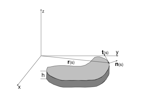
Figure 1: Schematic illustration of the slab geometry of a lipid domain, where $h$, $\mathbf{r}(s)$, $\mathbf{t}(s)$, $\mathbf{n}(s)$ are respectively the thickness of the domain, the displacement vector of any point in the boundary curve, the tangent and normal vectors of the point in the boundary curve.

III NUMERICAL METHOD

In the last section, we have derive the shape equation (6) of LMDs by using variational method. However, it is very hard to obtain its solutions. Here we will develop a numerical method to solve it. In terms of the physical meaning of variational method, we can express the force in the boundary curve in a vector form as

$$\mathbf{f}(s)=-\left\{\Delta P-\gamma\kappa(s)-(2\mu^{2}/{h}^{2})\oint dl[\hat{\mathbf{R}}_{ls}\times\mathbf{t}(l)][\sqrt{1+{({h}/{R})}^{2}}-1]\right\}\mathbf{n}.$$ (7)

Thus Eq.(6) reflects the force balance ($\mathbf{f}=0$) in the boundary curve.

We introduce a virtual damping system evolving with dynamical equation

$$\frac{\partial\mathbf{r}(s,\tau)}{\partial\tau}=\mathbf{f}(s),$$ (8)

where $\tau$ is virtual time. If a LMD whose boundary curve satisfies Eq.(6), its shape will keep unchange. On the contrary, $\mathbf{f}\neq 0$, the boundary curve will evolve according to Eq.(8). In a long enough time, a damping system can usually approach to a state satisfying $\partial\mathbf{r}/{\partial\tau}=0$ which implies $\mathbf{f}=0$. Thus the final configuration is naturally a solution to the shape equation (6). The above scheme to find numerical solutions of Eq.(6) is called the relaxation method, which had also been used to resolve hydrodynamics of the ferrofluid drop pattern formationA:S.A.Langer ; A:A.J.Dickstein ; A:D.P.Jackson , shape relaxation in Langmuir layersA:R.E.Goldstein and hydrodynamics of the monolayer problem at the air-water interfaceA:D.K.Lubensky by Goldstein and his collaborators.

In order to perform numerical calculations, we should transform the continuous equation (8) into the discrete form by dividing the boundary curve into $N$ segments with $N$ points and assuming the step of evolution time is $\tau_{0}$. Then we label $N$ points in the boundary as $1,2,\cdots,k-1,k,k+1,\cdots,N$ and the time sequence as $\tau_{0},2\tau_{0},\cdots,(j-1)\tau_{0},j\tau_{0},(j+1)\tau_{0},\cdots$. Eq.(8) is transformed into

$$\mathbf{r}_{j+1}^{k}-\mathbf{r}_{j}^{k}=\mathbf{f}_{j}^{k}\tau_{0},$$ (9)

where $\mathbf{f}_{j}^{k}$ is the discrete form of Eq.(7). The geometric quantities in this equation can be discreted as:

$$[ds]_{j}^{k} = |\mathbf{r}_{j}^{k+1}-\mathbf{r}_{j}^{k}|,$$ (10)

$$[\mathbf{t}]_{j}^{k} = \frac{\mathbf{r}_{j}^{k+1}-\mathbf{r}_{j}^{k}}{[ds]_{j}^{k}},$$ (11)

$$[\kappa\ \mathbf{n}]_{j}^{k} = \frac{\mathbf{t}_{j}^{k+1}-\mathbf{t}_{j}^{k}}{[ds]_{j}^{k}},$$ (12)

where $\mathbf{n}_{j}^{k}$ can be obtained by rotating $\mathbf{t}_{j}^{k}$ in $90^{\circ}$ clockwise.

The stop condition of our calculation of Eq.(9) is $\sum_{k=1}^{N}|\mathbf{r}_{J+1}^{k}-\mathbf{r}_{J}^{k}|<\epsilon$ for a large enough integer $J$ and a small enough number $\epsilon$.

IV RESULTS

IV.1 ANALYTICAL SOLUTIONS

IV.1.1 Circular solutions

For a circle with radius $R_{0}$, $\kappa=-\frac{1}{R_{0}}$. Because ${\hat{\bf R}}_{ls}$ and ${\bf t}(l)$ are unit vectors, we can respectively express them as $(\cos\theta_{ls},\sin\theta_{ls},0)$ and $(\cos\theta_{l},\sin\theta_{l},0)$. Eq. (6) is then transformed into:

$$ax+b=xE(2ix)-2x^{2}$$ (13)

where $x=\frac{R_{0}}{h}$, $a=\frac{\Delta Ph}{4\mu^{2}}$ , $b=\frac{\gamma}{4\mu^{2}}$, and $E(.)$ is complete elliptic integrals of the second kind.

From Fig 2, we find that a critical $a^{\ast}$ exists such that there are two solutions when $0<a<a^{\ast}$ and no solution when $a>a^{\ast}$. Additionally, there is only one solution for $a<0$ or $a=a^{\ast}$.

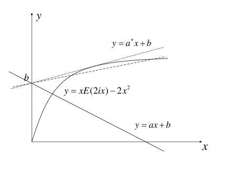
Figure 2: Schematic diagrams of functions $y=ax+b$ and $y=xE(2ix)-2x^{2}$. A critical $a^{\ast}$ exists so that there are two solutions when $0<a<a^{\ast}$ and no solution when $a>a^{\ast}$. Additionally, there is only one solution for $a<0$ or $a=a^{\ast}$.

In the limit case of $x\rightarrow\infty$, we have

$$xE(2ix)-2x^{2}\approx\frac{1}{4}\ln(8{\sqrt{e}}x),$$ (14)

from which we easily obtain the radius of the circular domain

$$R_{0}=\frac{e^{\frac{\gamma}{\mu^{2}}}}{8\sqrt{e}}h,$$ (15)

for vanishing $\Delta P$.

This result is similar to McConnell’s result

$$R_{0}=\frac{e^{3}e^{\frac{\gamma}{\mu}}}{4}\delta$$ (16)

with a cutoff $\delta$ A:H.M.McConnell88 .

IV.1.2 Toroidal solutions

Next, we investigate whether toroidal shapes are permitted in our model. The torus solution is mentioned in many referencesA:R.M.Weis85 ; A:H.M.McConnell90 ; A:M.Iwamoto04 ; A:M.Iwamoto06 . Here we only discuss the case of $h\ll min\{R_{1}-R_{2},R_{2}\}$, where $R_{1}$ and $R_{2}$ are the outer and inner radii, respectively.

From Eq. (6) we find the radii $R_{1}$ and $R_{2}$ should satisfy

$$\Delta PR_{1}+\gamma-\mu^{2}\ln\frac{8\sqrt{e}R_{1}}{h}+\mu^{2}\int_{0}^{2\pi}\frac{x(x-\cos\theta)d\theta}{(x^{2}+1-2x\cos\theta)^{\frac{3}{2}}}dl=0,$$ (17)

and

$$\Delta PR_{2}-\gamma+\mu^{2}\ln\frac{8\sqrt{e}R_{2}}{h}-\mu^{2}\int_{0}^{2\pi}\frac{x(1-x\cos\theta)d\theta}{(x^{2}+1-2x\cos\theta)^{\frac{3}{2}}}dl=0,$$ (18)

where $x=R_{2}/R_{1}$.

By adding Eq. (17) to Eq. (18), we obtain

$$\alpha(1+x)+\ln x-2[E(k)-K(k)]=0$$ (19)

where $\alpha=\frac{\Delta PR_{1}}{\mu^{2}}$, $k^{2}=-4x/(1-x)^{2}$. $K(k)$ and $E(k)$ are respectively complete elliptic integrals of the first kind and the second kind, respectively. As shown in Fig. 3, there is a critical solution $x\approx 0.182215$ when $\alpha\approx 2.525115$. This solution is close to the ratio $0.2$ observed in the experiment A:H.M.McConnell90 . For $\alpha>2.525115$ there are two toroidal solutions.

Therefore toroidal shapes are indeed permitted under certain conditions in our model.

Figure 3: Schematic diagram of function $f(x)=\alpha(1+x)+\ln x-2[E(k)-K(k)]$ when $\alpha\approx 2.525115$, there is a solution $x=R_{2}/R_{1}\approx 0.182215$.

IV.2 NUMERICAL SOLUTIONS

There are four parameters, $\mu^{2}$ , $\gamma$ , $h$ and $\Delta P$ in our model. We take the experimental values $h\approx 2nm$, $\mu^{2}=5\times 10^{-9}dyn$, and $\gamma=1.6\times 10^{-7}dyn$ A:D.J.Benvegnu . The surface energy density $\Delta P$ is an adjustable parameter, which can be understood as the Gibbs free energy difference between the fluid phase and solid phase A:M.Iwamoto04 .

To make sure of our numerical method, we consider the circular domains. The radius of circular domains is about $20\mu m$ in the experimentA:D.J.Benvegnu . Using the theoretical result Eq. (14), we obtain $\Delta P\approx-5.05255\times 10^{-5}dyn/cm$. Adopting this parameter in our simulations, we obtain stable circular domain with radius about $20\mu m$.

Now we use our numerical codes to search for various shapes of domains evolving from different initial configurations and $\Delta P$, and then compare them with the experimental results. After the long time calculations, we obtain heart form (Fig.4), S form (Fig.5), moon form (Fig.6) and dumbbell form (Fig.7) with adjustable parameters $\Delta P\approx 1.19338\times 10^{-4}dyn/cm$, $3.87582\times 10^{-3}dyn/cm$, $-1.42196\times 10^{-4}dyn/cm$, and $2.01274\times 10^{-4}dyn/cm$, respectively. These shapes and their sized are in good agreement with the experimentsA:Stine ; A:H.E.Gaub .

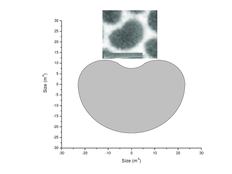
Figure 4: Smooth heart. The top figure is cut from Fig.5 (B) in Ref.A:Stine , where the bottom one is the numerical result with adjustable parameter $\Delta P\approx 1.19338\times 10^{-4}dyn/cm$.

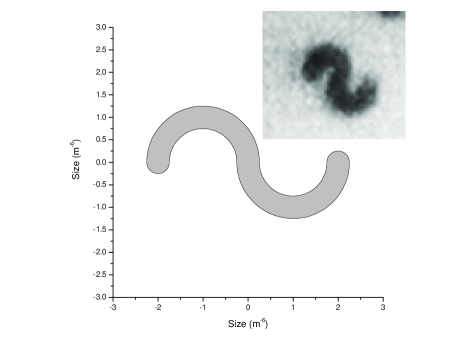
Figure 5: S domain. The figure in the top right hand corner is cut from the second picture of Fig.3 in Ref.A:H.E.Gaub , where the bottom left one is the numerical result with adjustable parameter $\Delta P\approx 3.87582\times 10^{-3}dyn/cm$.

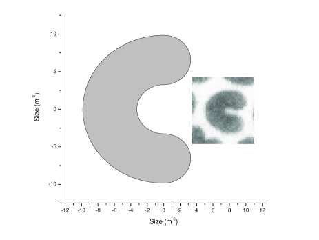
Figure 6: Moon. The right figure is cut from Fig.5 (D) in Ref.A:Stine , where the left one is the numerical result with adjustable parameter $\Delta P\approx-1.42196\times 10^{-4}dyn/cm$.

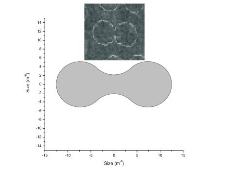
Figure 7: Dumbbell. The top figure is cut from Fig.1 in Ref.A:Stine , where the bottom one is the numerical result with adjustable parameter $\Delta P\approx 2.01274\times 10^{-4}dyn/cm$.

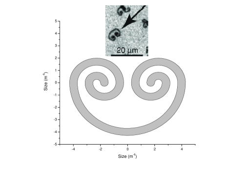
Figure 8: One-lobed domain. The top figure is cut from Fig.4 in Ref.A:Peter Kruger , where the bottom one is the numerical result with adjustable parameter $\Delta P\approx-3.97255\times 10^{-3}dyn/cm$.

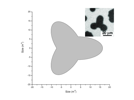
Figure 9: Three-leaves form without spiral arms. The figure in the top right hand corner is cut from the fifth picture of Fig.3 in Ref.A:Peter Kruger , where the bottom left one is the numerical result with adjustable parameter $\Delta P\approx-1.66338\times 10^{-4}dyn/cm$.

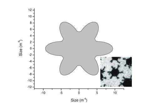
Figure 10: Smooth six-leaves form without spiral arms. The figure in the bottom right hand corner is cut from the second picture of Fig.3 in Ref.A:Peter Kruger99 , where the top left one is the numerical result with adjustable parameter $\Delta P\approx-3.11274\times 10^{-4}dyn/cm$.

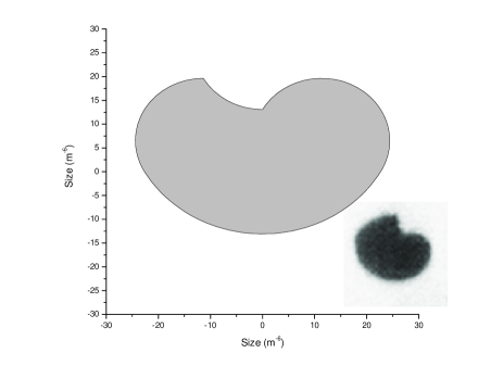
Figure 11: Bean with two cusps. The top figure in the bottom right hand corner is cut from the first picture of Fig.3 in Ref.A:H.E.Gaub , where the top left one is the numerical result with adjustable parameter $\Delta P\approx 9.94745\times 10^{-5}dyn/cm$.

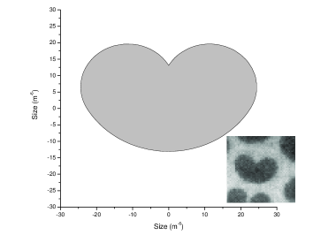
Figure 12: Heart with a cusp. The figure in the bottom right hand corner is cut from Fig.5 (D) in Ref.A:Stine , where the top left one is the numerical result with adjustable parameter $\Delta P\approx 9.72545\times 10^{-5}dyn/cm$.

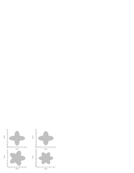
Figure 13: Multi-leaves forms. Top left, four-leaves form without cusps when $\Delta P\approx 1.63377\times 10^{-5}dyn/cm$. Top right, four-leaves form with cusps when $\Delta P\approx-2.06338\times 10^{-4}dyn/cm$. Bottom left, five-leaves form with cusps when $\Delta P\approx-8.63377\times 10^{-5}dyn/cm$. Bottom right, six-leaves form with cusps when $\Delta P\approx-1.34127\times 10^{-3}dyn/cm$.

In addition, our model can also obtain one-lobed domain (also called labyrinthine pattern) and three-leaves domain shown in Figs. 8 and 9 under the parameters $\Delta P\approx-3.97255\times 10^{-3}dyn/cm$ and $-1.66338\times 10^{-4}dyn/cm$, respectively. Their shapes and sizes are similar to those observed in Peter Krüger and Mathias Lösche’s experiment A:Peter Kruger .

Furthermore, we not only obtain a six-leaves form, which occurs in the experimentA:Peter Kruger99 in recent years, shown in Fig.10 with adjustable parameter $\Delta P\approx-3.11274\times 10^{-4}dyn/cm$, but also acquire some shapes with cusps observed in the experiments shown in Figs.11 and 12 with adjustable parameters $\Delta P\approx 9.94745\times 10^{-5}dyn/cm$ and $\Delta P\approx 9.72545\times 10^{-5}dyn/cm$, respectively. These results agree well with the experiments A:Stine ; A:H.E.Gaub .

Besides the shapes shown above, we can also produce some new stable shapes such as four-leaves, five-leaves, and six-leaves with cusps shown in Fig.13, which need to be verified by further biochemical experiments.

The amazing aspect in our results is that we can obtain some stable shapes with “cuspidal points”. Here the cusps are apparent ones viewed in the scale of micrometers. In our computational procedure, each cusps locally contain many discrete points in the scale of tens of nanometers such that the cusps are in fact the smooth curves. We find the average free energy per unit area of domains with cusps is less than those without cusps, that is, the former is stable than the latter. We show the bean shape, heart shape and multi-leaves shapes with cuspidal points in Figs.11, 12 and the last three pictures in Fig.13. In the latest theoretical work A:M.Iwamoto08 ; A:Iwamoto08 , Iwamoto et al. analytically prove that the existence of the cuspidal points is reasonable and there are two kinds of cusps, one’s curvature is positive, the other’s is negative. However, their method is a local theory, in which one equilibrium domain shape can produce only one type of cusp and the number is also one. Our theory is a global theory, because we directly calculate the double curve integrals and do not use any approximate expansion method. Through numerical simulation, we further find that two kinds of cusps can coexist in one equilibrium domain, as shown in Fig.11, in which there are two kinds of cusps. In fact, the domains with cusps have clearly been observed in serval experiments A:Stine ; A:H.E.Gaub ; A:D.K.Schwartz ; A:C.W.McConlogue . Thus the shapes with cuspidal points might be widespread in nature.

We have investigated various shapes of domains under different $\Delta P$. Now we draw a phase diagram in Fig. 14. It is found that the domain shape will become complex from the original circular domain when the parameter $\Delta P$ changes from $-5.05255\times 10^{-5}dyn/cm$ towards both ends of the coordinate axis. It seems that the domains with cusps generally occur in the narrow ranges of parameter $\Delta P$. Two shapes of domains can coexist in a certain interval, such as heart shape and dumbbell shape as shown in Figs.14, which agrees with the experimental observationsA:Stine ; A:H.E.Gaub that reveals some shapes can coexist under some parameters.

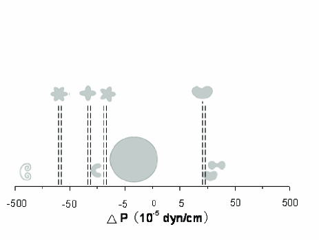
Figure 14: Phase diagram with various $\Delta P$ (in the Log coordinate).

V CONCLUSION

In the above discussions, we have theoretically and numerically investigated the shapes of planar lipid monolayer domains by minimizing the formation energy of the domains. We obtain some shapes, such as circular form, S form, dumbbell form, serpentine form and achiral multi-leaves form and so on. Most of them are observed in the experiments A:Stine ; A:H.E.Gaub ; A:Peter Kruger99 ; A:Peter Kruger . The four-leaves, five-leaves, and six-leaves forms await the future experimental conformations.

Our model might be extended to explain the shapes of rafts A:K.Simons consisting of sphingolipids and cholesterol in the cell membranes. Although the cell membrane is a bilayer, the raft domains are generally in one of the monolayers. There are net dipoles in the raft domains, thus our model might be applied to describe the shape of raft domains.

References

- (1) K.J. Stine, and D.T. Stratmann, Langmuir 8, 2509 (1992).
- (2) K.Y.C. Lee and H.M. McConnell, J. Phys. Chem. 97, 9532 (1993).
- (3) M.M. Lipp, K.Y.C. Lee, J.A. Zasadzinski, and A.J. Waring, Science 273, 1196 (1996).
- (4) R.M. Weis and H.M. McConnell, J. Phys. Chem. 89, 4453 (1985).
- (5) H.M. McConnell, P.A. Rice, and D.J. Benvegnu, J. Phys. Chem. 94, 8965 (1990).
- (6) R.M. Weis and H.M. McConnell, Nature 310, 47 (1984).
- (7) H.E.Gaub, V.T. Moy, and H.M. McConnell, J. Phys. Chem. 90, 1721 (1986).
- (8) P. Krüger, M. Schalke, Z. Wang, R.H. Notter, R.A. Dluhy, and M. Lösche, Biophys. J. 77, 903 (1999).
- (9) P. Krüger and M. Lösche, Phys. Rev. E 62, 7031 (2000).
- (10) H.M. McConnell and V.T. Moy, J. Phys. Chem. 92, 4520 (1988).
- (11) H.M. McConnell, J. Phys. Chem. 94, 4728 (1990).
- (12) M. Iwamoto and Z.C. Ou-Yang, Phys. Rev. Lett. 93, 206101 (2004).
- (13) M. Iwamoto, F. Liu, and Z.C. Ou-Yang, J. Chem. Phys. 125, 224701 (2006).
- (14) M. Iwamoto, F. Liu, and Z.C. Ou-Yang, Eur. Phys. J. E 27, 81 (2008).
- (15) M. Iwamoto, F. Liu, and Z.C. Ou-Yang, Int. J. Mod. Phys. B 22, 2047 (2008).
- (16) S.A. Langer, R.E. Goldstein, and D.P. Jackson, Phys. Rev. A 46, 4894 (1992).
- (17) Z.C. Tu and Z.C. Ou-Yang, J. Comput. Theor. Nanosci. 5, 422 (2008).
- (18) A.J. Dickstein, S. Erramilli, R.E. Goldstein, D.P. Jackson and S.A. Langer, Science 261, 1012 (1993).
- (19) D.P. Jackson, R.E. Goldstein and A.O. Cebers, Phys. Rev. E 50, 298 (1994).
- (20) R.E. Goldstein and D.P. Jackson, J. Phys. Chem. 98, 9626 (1994).
- (21) D.K. Lubensky and R.E. Goldstein, Phys. Fluids. 8, 843 (1996).
- (22) D.J. Benvegnu and H.M. McConnell, J. Phys. Chem. 96, 6820 (1992).
- (23) D.K. Schwartz, M.-W. Tsao, and C.M. Knobler, J. Chem. Phys. 101, 8258 (1994).
- (24) C.W. McConlogue and T.K. Vanderlick, Langmuir 13, 7158 (1997).
- (25) K. Simons and E. Ikonen, Nature 387, 569 (1997).