The spatial distribution of polar hydrogen deposits on the Moon

, ,

Abstract

A new analysis of the Lunar Prospector epithermal neutron data is presented, providing an improved map of the distribution of hydrogen near to the lunar poles. This is achieved using a specially developed pixon image reconstruction algorithm to deconvolve the instrumental response of the Lunar Prospector’s neutron spectrometer from the observed data, while simultaneously suppressing the statistical noise. The results show that these data alone require the hydrogen to be concentrated into the cold traps at up to 1 wt% water-equivalent hydrogen. This combination of localisation and high concentration suggests that the hydrogen is present either in the form of a volatile compound or as solar wind protons implanted into small regolith grains.

1 Introduction

Is there ice on the Moon? Finding the answer is important both for our understanding of the Solar System and for planning future visits. The fact that the Moon’s axis of rotation is inclined at only $1.6^{\circ}$ from the normal to the ecliptic means that permanently shaded regions exist inside many craters within $10^{\circ}$ of the lunar poles. These regions should be sufficiently cold ($<100$K) to prevent significant sublimation of water ice over billions of years (Vasavada et al., 1999). The flux of water reaching the Moon via impacts with comets and meteorites and subsequently able to migrate to the relative safety of the polar ‘cold traps’ should be significant over the age of the solar system (Arnold, 1979; Crider and Vondrak, 2003; Butler, 1997). Hydrogen delivered by the solar wind can also create water by chemical reduction of the lunar regolith, providing another potential source of polar ice (Arnold, 1979; Crider and Vondrak, 2000).

While the existence of ice on the Moon was considered in the 1960s (Watson et al., 1961), interest was rekindled in the 1990s, when two different methods were employed to address the issue, namely radar reflection experiments and neutron spectroscopy from Lunar Prospector. The radar method relies upon detecting the preferential reflection of the same sense of circular polarisation carried by the incident radiation. This coherent backscatter opposition effect could result from volume scattering within a largely transparent medium, such as reasonably pure ice (Hapke, 1990). However, lunar observations have shown that same-sense circularly polarised radio waves are preferentially returned even from sunlit locations (Stacy et al., 1997; Simpson and Tyler, 1999; Campbell et al., 2006; Campbell and Campbell, 2006), making the most plausible explanation that this is surface scattering from blocky ejecta within craters, rather than volume scattering from large chunks of ice.

The strongest evidence for water ice at the poles is provided by the deficit in the epithermal (0.3eV-100keV) neutron counts detected by the Lunar Prospector. Cosmic rays impacting upon nuclei in the regolith liberate neutrons. These elastically and inelastically scatter off nuclei in the top few metres of the lunar regolith and some leak out of the surface before they suffer nuclear capture or spontaneously decay. Adding hydrogen to the regolith means that kinetic energy is more rapidly drained from the neutrons during elastic collisions. Consequently, fewer epithermal neutrons escape to be detected by orbiting neutron spectrometers. Thus, a deficit of epithermal neutrons is produced when there is a concentration of hydrogen in the top $\sim 1$ metre of the regolith (Feldman et al., 1991).

Lunar Prospector’s neutron spectrometer detected a significant dip in the epithermal neutron count rate over both lunar poles, suggesting an excess of hydrogen in these areas (Feldman et al., 1998, 2000, 2001). These tantalising results did not definitively determine whether or not the hydrogen was confined to the cold traps. If the excess hydrogen were distributed throughout the polar regions, then it could just be solar wind-implanted protons bound in OH groups that were less likely to diffuse out of the locally cold regolith (Starukhina and Shkuratov, 2000). Even if the hydrogen were confined to the cold traps, then the temperatures should be low enough that regolith grains will retain some free H atoms. Feldman et al. (2001) studied this in detail, concluding that the diffusivity of hydrogen was unlikely to be relevant within cold traps. When trying to discriminate between these various possible forms for the excess polar hydrogen, it would clearly be helpful to know whether or not it is confined to the permanently shaded regions, and how concentrated this hydrogen is.

2 Pixon Image Reconstruction

Earlier studies of the Lunar Prospector data have used either the high-altitude (100 km) epithermal data (Feldman et al., 1998) or smoothed versions of the low-altitude (30 km) data (Feldman et al., 2000, 2001). The response of the Lunar Prospector has a FWHM of 130 km and 45 km for high and low altitude orbits respectively. To determine whether or not the hydrogen is confined to the cold traps requires an approach that deconvolves the Lunar Prospector data while not introducing spurious complexity. This is the usual challenge in image reconstruction. Namely, given an input two-dimensional map, $I$, which is measured with an instrument that blurs it through a response function, $B$, and introduces some random noise, $N$, then the measured data satisfies

$$D=I*B+N.$$ (1)

The inclusion of noise means that the best that can be achieved is that the inferred image, ${\hat{I}}$, avoids unnecessary complexity and produces a residual field,

$$R=D-{\hat{I}}*B,$$ (2)

that is statistically equivalent to the anticipated noise, $N$.

The standard way to approach this problem is to consider the following equation concerning conditional probabilities:

$$p({\hat{I}},M|D)=\frac{p(D|{\hat{I}},M)p({\hat{I}}|M)p(M)}{p(D)}.$$ (3)

$M$ represents all aspects of the model for transforming the inferred image, ${\hat{I}}$, to the data, $D$. This includes the assumed response function, $B$, the pixellisation of the data and the assumed characteristics of the noise. $p(D)$ is a constant, and, to avoid introducing prejudice, so is $p(M)$. Thus,

$$p({\hat{I}},M|D)\propto p(D|{\hat{I}},M)p({\hat{I}}|M).$$ (4)

The term on the left-hand side of this proportionality is commonly known as the posteriori probability, $P_{\rm post}\equiv p({\hat{I}},M|D)$, which should be maximised by the reconstruction. The two terms on the right are the likelihood ($p(D|{\hat{I}},M)\equiv e^{-0.5\chi^{2}}$ for the usual definition of the $\chi^{2}$ goodness-of-fit statistic) and the image prior, $P_{IP}\equiv p({\hat{I}}|M)$, respectively. The likelihood increases as the complexity of the reconstructed image, ${\hat{I}}$, is increased and the fit to the data improves. In contrast, the image prior decreases with increasing complexity in ${\hat{I}}$. This means that the optimal reconstruction (maximum $P_{\rm post}$) occurs at the point where increasing complexity in the reconstruction no longer improves the fit sufficiently to be justified by the information content in the data.

A particularly suitable method for maximising the posteriori probability is the pixon image reconstruction algorithm (Pina and Puetter, 1993; Eke, 2001). A pixon can be thought of as a collection of pixels carrying a particular amount of information. Thus, the reconstruction of the Lunar Prospector data, which is well-sampled at the lunar poles and less so further away due to the polar orbit of the spacecraft, will have many small pixons to describe ${\hat{I}}$ near to the pole, and a few larger pixons where the signal-to-noise ratio decreases at lower latitudes. ${\hat{I}}$ is constructed by convolving a pseudoimage, defined in the pixel array and constrained to lie within physically acceptable count rates, with a position-dependent kernel, whose width represents the local pixon size. The optimum reconstruction is the one that combines simplicity of the reconstructed image with an acceptable residual field.

2.1 Choosing the optimum number of pixons

In order to determine the optimum number of pixons, $n_{\rm p}$, required to reconstruct an image, the total information in the data set is first determined via

$$\Upsilon=\sum_{\bf x}\frac{n_{\rm n}({\bf x})}{\alpha\sqrt{n_{\rm n}({\bf x})}}=\sum_{\bf x}\upsilon({\bf x}),$$ (5)

where $n_{\rm n}({\bf x})$ is the number of neutrons in pixel x, and $\upsilon({\bf x})=\sqrt{n_{\rm n}({\bf x})}/\alpha$ is the signal-to-noise ratio in pixel x. Note that the choice of $\alpha$ is somewhat arbitrary. How many $\sigma$ should a signal be before it counts as a piece of information? A value of $\alpha=2$ has been chosen, although no significant change is made to the reconstruction by choosing $\alpha=1$.

To maximise the entropy of the reconstruction, the information placed into each pixon should be the same. Thus, for a given total number of pixons in the reconstruction, each should contain $\Upsilon/n_{\rm p}$ pieces of information. The Gaussian pixon, $K_{\bf x}$, was selected for each pixel such that

$$\upsilon*K_{\bf x}=\Upsilon/n_{\rm p}.$$ (6)

With the pixon distribution set for a particular total number of pixons, the algorithm then uses the Fletcher-Reeves conjugate gradient algorithm to minimise $E_{r}$, the autocorrelation of the reduced residuals ($r=R/\sigma$) statistic (Pina and Puetter, 1992), applied for lags of 1 pixel. Having thus found the best fit for this number of pixons, the posteriori probability, $P_{\rm post}$, can be calculated by multiplying together the likelihood ($e^{-0.5\chi^{2}}$) and the image prior, which is

$$P_{IP}=\frac{\Upsilon!}{n_{\rm p}^{\Upsilon}\left[\left(\frac{\Upsilon}{n_{\rm p}}\right)!\right]^{n_{\rm p}}}.$$ (7)

Using Stirling’s approximation gives

$${\rm ln}(P_{\rm post})\approx 0.5[{\rm ln}\Upsilon+(1-n_{\rm p}){\rm ln}(2\pi)-n_{\rm p}{\rm ln}(\Upsilon/n_{\rm p})-\chi^{2}].$$ (8)

Thus, the number of pixons that maximises ${\rm ln}(P_{\rm post})$ can be found, and this provides the optimal reconstruction.

2.2 Coupled and decoupled reconstructions

The reconstructed image, $\hat{I}$, is defined by gathering signal from a pseudoimage, $W$. This gathering amounts to a convolution of the pseudoimage with the normalised pixon kernel appropriate for each pixel, namely

$$\hat{I}({\bf x})=W*K_{\bf x}.$$ (9)

Constraints are placed on $W$, so that it cannot take unphysical values, such as count rates less than zero or greater than 22 epithermal neutrons per second, which is larger than the rate expected from regolith containing no hydrogen whatsoever (Lawrence et al., 2006). A set of 11 Gaussian pixons, with widths varying from $10$ km to $250$ km are available for the algorithm to choose. When a single pseudoimage is employed, the sunlit and permanently shaded pixels are treated equally. This is termed a coupled reconstruction. However, one should include some prior knowledge that sunlit pixels would not be expected to have a hydrogen content exceeding a few times that in the returned lunar samples. A loose limit of $15$ counts per second is chosen for the minimum allowable epithermal rate in sunlit pixels. Introducing an independently determined map of permanently shaded pixels enables a decoupled treatment of the two types of pixel; sunlit and shadow. Each pixel type has its own pseudoimage, with different limits on their allowed count rates: sunlit - [15,22] and shadow - [0,22]. These pseudoimages only have non-zero elements for pixels of the type being considered. Thus, to avoid having the pseudoimage grow to compensate for this near to the boundaries between pixel types, a mask, $m_{\rm type}({\bf x})$, of ones and zeros is set up for each pixel type, with the ones lying only in pixels of the chosen type. This mask is then convolved with the appropriate pixon kernel for each pixel to give a map of weights

$$M_{\rm type}=m_{\rm type}*K_{\bf x}.$$ (10)

The resulting map, $M_{\rm type}$, has values lying in the range $(0,1]$ and can be used to define the decoupled reconstruction via

$$\hat{I}=\frac{(W_{\rm type}*K_{\bf x})}{M_{\rm type}}.$$ (11)

In practice because the required pixon size is a continuous variable, whereas only a finite set of distinct pixon sizes are actually used, the reconstruction is created by interpolating between the nearest two available pixon kernels. By decoupling the shadow and sunlit pixel values, the effective number of pixons being used increases. To account for this, $n_{\rm p}$ is replaced in the image prior calculation by $n_{\rm p}~{}G$, where

$$G=\frac{1}{n_{\rm pixel}}\sum_{\bf x}\frac{1}{M_{\rm type}({\bf x})}~{},$$ (12)

with the sum being over all $n_{\rm pixel}$ pixels ${\bf x}$.

Note that, for the decoupled reconstructions of the real data, the sunlit pixels take values in the ranges [18.5,20.5] counts per second for the north pole, and [18.3,20.7] counts per second for the south pole. For the north pole, this range corresponds to plausible amounts of hydrogen for occasionally sunlit terrain. The construction of the north and south pole shadow maps is described in detail by Elphic et al. (2007). In brief, radar tomographic maps (Margot et al., 1999; U.S. Geological Survey, 2002) were combined with the model of polar craters produced by Bussey et al. (2003). Gaps were filled by interpolation and the whole resulting landscape was projected on a sphere of 1738 km radius, and illuminated with summer sunlight. Note that the permanently shaded areas are better determined around the north pole because the south pole shadow map was largely derived from data taken during winter lighting conditions (Elphic et al., 2007). The less well determined shadow map in the south may be behind the larger range of values being used by the sunlit pixels in this case.

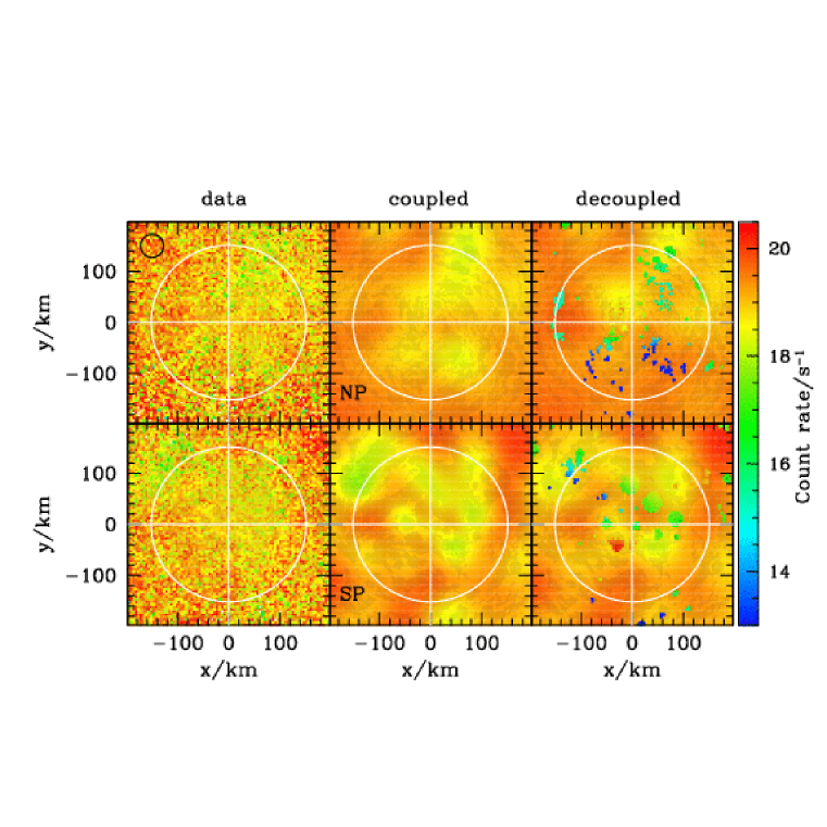
Figure 1: Epithermal count rate maps for the north (top row) and south (bottom row) poles. From left to right, the columns represent the data, $D$, the coupled and decoupled reconstructions, $\hat{I}$. The white circles represent a latitude of $\pm 85^{\circ}$ and the shading shows Clementine imaging. Also shown, with a black circle in the top left panel is the size of the Lunar Prospector’s PSF. The spherical surface has been represented in these panels such that the distance from the image centre represents the arc length to the pole, and, following convention, $0^{\circ}$ longitude points down/up for the north/south poles respectively.

The left hand panels of Fig1 show the north (top) and south (bottom) pole epithermal data. These can be contrasted with the central and right hand columns in Fig1, showing ${\hat{I}}$ from two different reconstructions of both data sets. These four reconstructions all provide residual fields with acceptable $\chi^{2}$ values, and differ only because an additional shadow map prior was included for the decoupled reconstructions in the right hand column, unlike the coupled reconstructions in the central column. The coupled reconstructions are very similar to the count rate maps created by merely smoothing the observational data using a Gaussian with FWHM of 40 km, as chosen by Feldman et al. (2001). The decoupling significantly changes the inferred hydrogen abundance within the cold traps, which are clearly visible because of the rapid count rate jumps across their edges. If a good fit is defined merely using $\chi^{2}$, then there appears to be no need to impose the shadow map. The coupled reconstruction is simpler too, so the use of the shadow map can only be justified if the data demand it.

3 Results

The coupled and decoupled reconstructions differ significantly only in the epithermal neutron count rates present in the cold traps. Thus, the residuals in the vicinity of these permanently shaded areas offer the best route to determine if the data contain sufficient information to discriminate between these two different reconstructions. If a real count rate dip in a cold trap were wrongly smoothed over in the reconstruction, then one would expect to see a radial variation in the mean residual moving out from the cold trap centre. The pattern of these spatially correlated residuals would depend upon the size of the cold trap, the depth of the count rate dip, and the FWHM of the instrumental response.

3.1 The radial dependence of the mean stacked residuals

In order to try and discriminate between the two types of reconstruction, it is desirable to stack together the residuals around all sufficiently large (at least 3 contiguous pixels) cold traps. From the right hand panels in Fig1, it is clear that the cold traps have a variety of sizes and shapes, and that they are often sufficiently close to one another that the anticipated rings of non-zero residuals around them would overlap. In the face of these complications, the easiest way to understand the significance of the results is to use a Monte Carlo method, whereby mock data sets are created and then analysed in exactly the same way as the real data itself. To this end, 100 different noisy mock Lunar Prospector time series data sets were created, taking the reconstructions in Fig1 as the input images, $I(\bf x)$. The different mocks varied only as a result of the random numbers chosen to add the noise. Both coupled and decoupled reconstructions were performed, and the stacked radial profiles of the reduced residuals, $r=R/\sigma$ with $\sigma$ coming from counting statistics, around cold trap centres were calculated. Pixels positioned near to more than one permanently shaded region were only counted once, at the radius appropriate for the nearest cold trap.

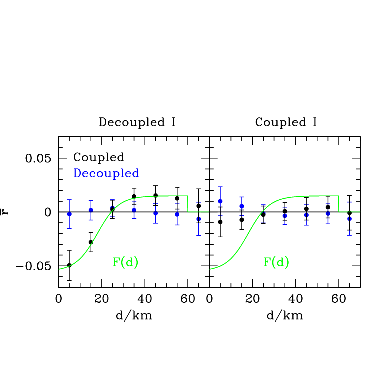
Figure 2: The variation of the mean reduced residual per observation, ${\bar{r}}$, with the distance to the centre of the nearest permanently shaded crater, $d$. The results are stacked for all permanently shaded areas in both the north and south polar regions containing at least 3 contiguous shadow pixels. Coupled (black) and decoupled (blue) reconstructions are shown in both panels. The left hand panel shows reconstructions from mock data made with the decoupled reconstruction of the real data as the input image. Error bars represent the $1\sigma$ scatter between the individual mock results. The green curve represents the function $F(d)$ given in Eq. 14, which is a fit to the results from the coupled reconstructions. The right hand panel shows the results for mocks made using the coupled reconstructions of the real data, shown in the central column of Fig1, as the input image for the 100 mock catalogues.

The left hand panel in Fig2 shows the radial dependence of the reduced residuals for both types of reconstruction of the mocks created from the decoupled reconstructions of the real data. Error bars represent the $1\sigma$ scatter between the results obtained from the individual mock data sets. The decoupled reconstructions show no radial trend in the mean reduced residual around the cold traps, which contrasts with the results from the coupled reconstructions. These show a negative residual for distances less than $\sim 25$ km, swapping over to a positive one at larger radii, signifying that ${\hat{I}}$ is too large in the cold traps. While the global $\chi^{2}$ may be acceptable, the coupled reconstruction produces spatially correlated residuals near to cold traps. To remove these would require either a vastly increased number of pixons, which would produce a hugely detailed and improbable reconstruction, or the imposition of a shadow map. In short, these mock Lunar Prospector epithermal neutron data sets contain sufficient information to distinguish between the coupled and decoupled reconstructions, i.e. the real data should tell us if the excess hydrogen is concentrated into the cold traps or more diffusely distributed.

The right hand panel in Fig2 shows how the mean reduced residuals vary when the pixon algorithm is applied to mock data sets constructed from the input image where the count rate dips are not localised to the crater, i.e. the coupled reconstruction of the real data. It is apparent that there is a small bias, whereby the decoupled reconstruction still tries to put a slight count rate dip into the cold traps where it is not actually present. Also, the coupled reconstruction tends to oversmooth the small dips that did exist. However, these systematic biases resulting from the method are negligible relative to the size of the deviations found in the case of the decoupled input image.

Fig3 shows the corresponding information for the coupled and decoupled reconstructions of the real data, with the error bars now representing the error on the mean reduced residual. A very similar pattern in the residuals is seen, for all but the central bin, as was the case for the mock reconstructions made using the decoupled input image. There are relatively few pixels, and hence observations, contributing to the central bin, which nevertheless still lies in the tail of the distribution of the mock results. Just as for the mock reconstructions, including the independently determined shadow map removes the correlated residuals out to $60$ km from the cold trap centres. Thus, the Lunar Prospector data are not adequately described by the coupled reconstruction, and they do require that the epithermal count rate dips are concentrated into the permanently shaded regions.

3.2 Shadowiness

The results in the previous subsection imply that the Lunar Prospector epithermal neutron data themselves pick out the pixels that should be cold traps. In this section, the same conclusion is reached in a more quantitative way without resorting to stacking together the disparate cold traps. Consider a shadowiness parameter $S$ defined via

$$S=r*F,$$ (13)

where the filter function $F$, shown by the green curve in Fig2, is given by

$$F(d)=\left\{\begin{array}[]{lll}0.035~{}{\rm tanh}\left(\frac{(d/{\rm km})-18}{10}\right)-0.02&{}{}{}&d\leq 60~{}{\rm km};\\ 0&&d>60~{}{\rm km}.\\ \end{array}\right.$$ (14)

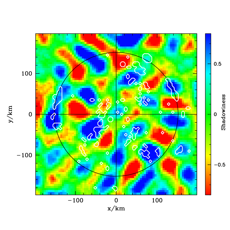
Figure 4: The shadowiness map for the coupled reconstruction of the north pole Lunar Prospector data. Cold traps are outlined in white, and these can be seen to lie preferentially in regions of high shadowiness according to the neutron data.

$F(d)$ is merely a function that represents the radial dependence of the spatial correlations in the reduced residuals when a coupled reconstruction is performed on a data set derived from an input image where the hydrogen is concentrated into shaded areas. For spatially uncorrelated residuals, the distribution of $S$ should have a median of zero. A significantly positive median value would imply that the reconstruction is systematically overestimating the count rate in that set of pixels. A map of the shadowiness parameter is shown in Fig4 for the coupled reconstruction of the real north pole data, where the shadow map prior is relatively well known. The locations of the independently determined shadow pixels are superimposed in white. Areas of high shadowiness, shown in blue, tend to coincide with the permanently shaded regions.

Fig5 shows the cumulative distributions of shadowiness for a random reduced residual field, and for the shadow pixels for a number of different coupled reconstructions. The points show the mean distribution recovered from 100 mocks made using either the decoupled (circles) or coupled (crosses) input north pole image. Error bars represent the standard deviation between the mock reconstructions. The long-dashed line is the distribution for the real north pole shadow pixels. If the shadowiness parameter and the shadow map were truly uncorrelated, then this cumulative distribution of $S$ would be indistinguishable from that resulting from the randomly distributed residuals. This is not the case, implying that the Lunar Prospector data have picked out as special, in a statistical sense, the pixels that are independently known to be permanently shaded. While not as convincing, perhaps as a result of the less well determined shadow map, the south pole results have also been added with a short-dashed line.

3.3 Uncertainties in the reconstructions

While the stacked reduced residuals from all north and south pole shaded regions contain enough information to determine whether or not the count rate dips are typically concentrated into the cold traps, it is also interesting to know what is the uncertainty on the mean count rate within any individual cold trap. Permanently shaded regions that received more observations, either as a result of being large or near to the poles, will have better constrained mean epithermal neutron count rates. One would really like to know, given the measured cold trap count rates, what is the probability distribution of the true count rates. The mock catalogues allow two slightly different, yet closely related, questions to be answered, namely:
1. if the hydrogen is as concentrated as the decoupled reconstruction of the real data suggests, then what are the bias and scatter in the decoupled reconstruction values, and
2. if the hydrogen is as diffuse as the coupled reconstruction of the real data suggests, then what is the probability that a decoupled reconstruction will yield a cold trap count rate at least as low as did that from the decoupled reconstruction of the real data.
Table 1 contains this information, calculated from the appropriate set of 100 mocks for a few notable craters. From these data, it appears as if the north pole contains permanently shaded areas with deeper dips, i.e. more convincing hydrogen excesses, than exist in the south. An epithermal count rate of $\sim 13.5$ per second corresponds to $1$ wt% water-equivalent hydrogen (Lawrence et al., 2006).

3.4 Discussion

The results presented in this section demonstrate that:
1. the Lunar Prospector epithermal neutron data rule out the hypothesis that the hydrogen concentration is smoothly distributed in the polar regions, and
2. the set of permanently shadowed pixels defined by the shadow maps of Elphic et al. (2007) is statistically picked out as special.
The first of these statements follows from the fact that spatially correlated residuals result if one assumes that the hydrogen distribution is smoothly distributed throughout the polar regions. These statistically unacceptable residuals are evident in both Fig3 and Fig5. Over most of the reconstructed image, the residuals are statistically acceptable and spatially uncorrelated. However, these figures show the problem because they focus on the residuals in the vicinity of a particular set of pixels, namely those that are deemed to harbour regions of permanent shade. The information content latent within the data is sufficient to reject the hypothesis that the hydrogen is smoothly distributed, but one needs to know where to look to discover this message. The shadow map merely acts to focus attention into the regions where the useful information resides. If a random set of pixels were chosen as centres around which to investigate the residuals, then these correlations would not be seen. In fact, mapping the south pole shadow map pixel locations onto the north pole data and looking at the residuals around this different set of pixels shows no problem at all. The shadowiness distribution is completely consistent with that expected if the residuals were really random and spatially uncorrelated. Similarly, the residuals around a set of pixels in north pole craters supposedly without areas of permanent shade also show no deviations from the results that true randomly distributed residuals would produce. These observations illustrate the second statement above. The areas that are independently thought to harbour permanent shade lie preferentially in regions where the smoothly-distributed hydrogen reconstruction produces spatially correlated residuals. The simplest, and only plausible, way to remove these local correlations in the residuals is to concentrate the hydrogen into the cold trap pixels.

4 Conclusions

This study shows that the Lunar Prospector data alone require the polar hydrogen excess to be concentrated into the permanently shaded cold traps, rather than being more diffusely distributed. In some craters the concentration of hydrogen is sufficiently high that it corresponds to $\sim 1$ wt% water. This combination of localisation into the permanently shaded polar craters and consequent relatively high concentration is consistent with the hypothesis that the hydrogen is present in the form of water ice. However, these concentrations are not sufficiently high to preclude the hydrogen being in the form of solar wind protons implanted into regolith grains (Feldman et al., 2001). While the Lunar Prospector data are not able to determine the intracrater distribution of hydrogen, radar results suggest that it is unlikely to be concentrated into small patches of high purity water ice, at least not in the regions of the cold traps accessible to Earth-based detectors. Assuming that the excess hydrogen is in the form of water ice that reaches 2 m into the regolith, the depth expected to be gardened in 2 billion years (Feldman et al., 2001), this suggests that there are a few times $10^{11}$kg of water ice within permanently shaded regions within $10^{\circ}$ of the lunar poles.

Mean epithermal neutron count rates and their uncertainties for a few notable locations
Crater Location $d$ $c$ $d_{\rm mock}\pm 1\sigma$ $P(\leq d|c)$ Cabaeus $84.5^{\circ}{\rm S},322^{\circ}{\rm E}$ $14.8$ $18.1$ $14.1\pm 1.1$ $0.04$ de Gerlache $88.5^{\circ}{\rm S},273^{\circ}{\rm E}$ $16.8$ $18.5$ $17.5\pm 0.8$ $0.22$ Faustini $87.3^{\circ}{\rm S},77^{\circ}{\rm E}$ $17.2$ $18.4$ $17.0\pm 0.7$ $0.22$ Shackleton $89.7^{\circ}{\rm S},110^{\circ}{\rm E}$ $16.7$ $18.8$ $18.8\pm 0.5$ $<0.01$ Shoemaker $88.1^{\circ}{\rm S},45^{\circ}{\rm E}$ $17.8$ $18.7$ $18.4\pm 0.4$ $0.01$ Unnamed $89.2^{\circ}{\rm N},36^{\circ}{\rm E}$ $10.5$ $18.6$ $10.0\pm 1.3$ $<0.01$ Unnamed $89.6^{\circ}{\rm N},45^{\circ}{\rm E}$ $13.8$ $18.7$ $12.8\pm 1.1$ $0.01$

Table 1: The decoupled, $d$, and coupled, $c$, reconstruction mean cold trap epithermal neutron count rates are listed, in counts per second, along with the mean and scatter of the decoupled reconstructions of the decoupled mocks, $d_{\rm mock}$, and the probability of measuring a value at least as low as $d$, when doing a reconstruction of an image where the true value is $c$.

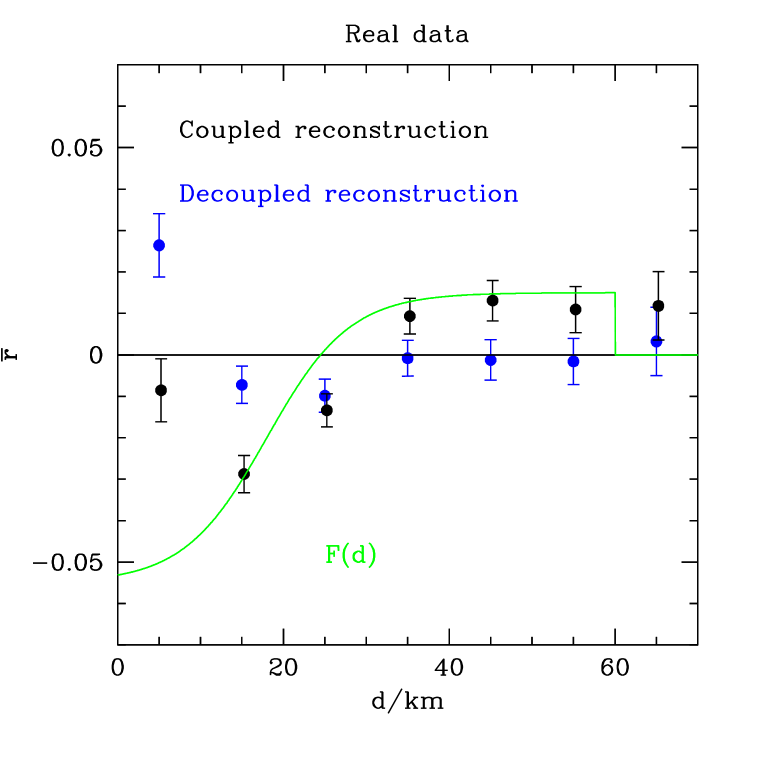
Figure 3: As for Fig2, using the stacked reduced residuals around cold traps for reconstructions of the real data. Error bars represent the errors on the mean reduced residuals.

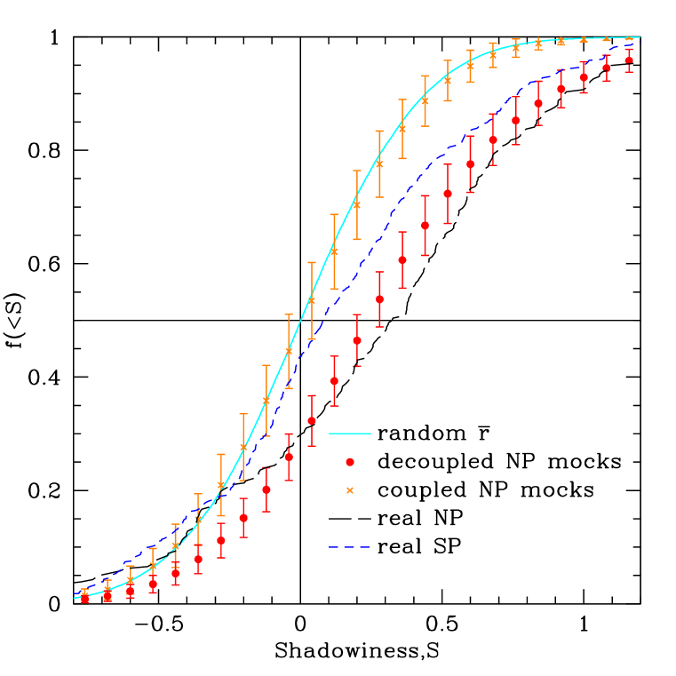
Figure 5: Shadowiness distributions for various coupled north pole reconstructions. Points show mean results from 100 mock data sets made using either the coupled (crosses) or decoupled (circles) input image. Error bars represent the standard deviation between the mock distributions. The distributions of the mock results are accurately represented by Gaussians. Results from the north and south pole reconstructions of the real data are shown by long- and short-dashed lines respectively. A solid line shows what the shadowiness distribution looks like for an uncorrelated random Gaussian residual field with $\sigma=1$.

References

- Arnold (1979) Arnold, J. R., Sep. 1979. Ice in the lunar polar regions. J. Geophys. Res. 84, 5659–5668.
- Bussey et al. (2003) Bussey, D. B. J., Lucey, P. G., Steutel, D., Robinson, M. S., Spudis, P. D., Edwards, K. D., Mar. 2003. Permanent shadow in simple craters near the lunar poles. Geophys. Res. Lett. 30 (6), 060000–1.
- Butler (1997) Butler, B. J., Aug. 1997. The migration of volatiles on the surfaces of Mercury and the Moon. J. Geophys. Res. 102, 19283–19292.
- Campbell and Campbell (2006) Campbell, B. A., Campbell, D. B., Jan. 2006. Regolith properties in the south polar region of the Moon from 70-cm radar polarimetry. Icarus 180, 1–7.
- Campbell et al. (2006) Campbell, D. B., Campbell, B. A., Carter, L. M., Margot, J.-L., Stacy, N. J. S., Oct. 2006. No evidence for thick deposits of ice at the lunar south pole. Nature 443, 835–837.
- Crider and Vondrak (2000) Crider, D. H., Vondrak, R. R., Nov. 2000. The solar wind as a possible source of lunar polar hydrogen deposits. J. Geophys. Res. 105, 26773–26782.
- Crider and Vondrak (2003) Crider, D. H., Vondrak, R. R., Jun. 2003. Space weathering of ice layers in lunar cold traps. Advances in Space Research 31, 2293–2298.
- Eke (2001) Eke, V., Jun. 2001. A speedy pixon image reconstruction algorithm. Mon. Not. R. Astron. Soc. 324, 108–118.
- Elphic et al. (2007) Elphic, R. C., Eke, V. R., Teodoro, L. F. A., Lawrence, D. J., Bussey, D. B. J., Jul. 2007. Models of the distribution and abundance of hydrogen at the lunar south pole. Geophys. Res. Lett. 34, L13204.
- Feldman et al. (2000) Feldman, W. C., Lawrence, D. J., Elphic, R. C., Barraclough, B. L., Maurice, S., Genetay, I., Binder, A. B., Feb. 2000. Polar hydrogen deposits on the Moon. J. Geophys. Res. 105, 4175–4196.
- Feldman et al. (1998) Feldman, W. C., Maurice, S., Binder, A. B., Barraclough, B. L., Elphic, R. C., Lawrence, D. J., Sep. 1998. Fluxes of Fast and Epithermal Neutrons from Lunar Prospector: Evidence for Water Ice at the Lunar Poles. Science 281, 1496–1500.
- Feldman et al. (2001) Feldman, W. C., Maurice, S., Lawrence, D. J., Little, R. C., Lawson, S. L., Gasnault, O., Wiens, R. C., Barraclough, B. L., Elphic, R. C., Prettyman, T. H., Steinberg, J. T., Binder, A. B., Oct. 2001. Evidence for water ice near the lunar poles. J. Geophys. Res. 106, 23231–23252.
- Feldman et al. (1991) Feldman, W. C., Reedy, R. C., McKay, D. S., Nov. 1991. Lunar neutron leakage fluxes as a function of composition and hydrogen content. Geophys. Res. Lett. 18, 2157–2160.
- Hapke (1990) Hapke, B., Dec. 1990. Coherent backscatter and the radar characteristics of outer planet satellites. Icarus 88, 407–417.
- Lawrence et al. (2006) Lawrence, D. J., Feldman, W. C., Elphic, R. C., Hagerty, J. J., Maurice, S., McKinney, G. W., Prettyman, T. H., Aug. 2006. Improved modeling of Lunar Prospector neutron spectrometer data: Implications for hydrogen deposits at the lunar poles. Journal of Geophysical Research (Planets) 111, E08001.
- Pina and Puetter (1992) Pina, R. K., Puetter, R. C., Nov. 1992. Incorporation of Spatial Information in Bayesian Image Reconstruction: The Maximum Residual Likelihood Criterion. Publ. Astron. Soc. Pac. 104, 1096–1103.
- Pina and Puetter (1993) Pina, R. K., Puetter, R. C., Jun. 1993. Bayesian image reconstruction - The pixon and optimal image modeling. Publ. Astron. Soc. Pac. 105, 630–637.
- Simpson and Tyler (1999) Simpson, R. A., Tyler, G. L., Feb. 1999. Reanalysis of Clementine bistatic radar data from the lunar South Pole. J. Geophys. Res. 104, 3845–3862.
- Stacy et al. (1997) Stacy, N. J. S., Campbell, D. B., Ford, P. G., 1997. Arecibo radar mapping of the lunar poles: A search for ice deposits. Science 276, 1527–1530.
- Starukhina and Shkuratov (2000) Starukhina, L. V., Shkuratov, Y. G., Oct. 2000. NOTE: The Lunar Poles: Water Ice or Chemically Trapped Hydrogen? Icarus 147, 585–587.
- Vasavada et al. (1999) Vasavada, A. R., Paige, D. A., Wood, S. E., Oct. 1999. Near-Surface Temperatures on Mercury and the Moon and the Stability of Polar Ice Deposits. Icarus 141, 179–193.
- Watson et al. (1961) Watson, K., Murray, B., Brown, H., May 1961. On the Possible Presence of Ice on the Moon. J. Geophys. Res. 66, 1598–1600.