Strangeness and glue in the nucleon from lattice QCD

Abstract:

We study the strangeness contribution to nucleon matrix elements using $N_{f}=2+1$ dynamical clover fermion configurations generated by the CP-PACS/JLQCD collaboration. In order to evaluate the disconnected insertion (DI), we use the Z(4) stochastic method, along with unbiased subtraction from the hopping parameter expansion which reduces the off-diagonal noises in the stochastic method. Furthermore, we find that using many nucleon sources for each configuration is effective in improving the signal. Our results for the quark contribution to the first moment $\xnuc_{q}$ in the DI, and the strangeness magnetic moment show that the statistical errors are under control with these techniques. We also study the gluonic contribution to the nucleon using the overlap operator to construct the gauge field tensor, $F_{\mu\nu}$. The application to the calculation of first moment, $\xnuc_{G}$, gives a good signal in quenched lattice QCD.

1 Introduction

The understanding of the structure of nucleon is one of the central issues in hadron physics. For instance, the parton distribution functions (PDFs) have been studied extensively, and the observation of scaling violation in PDFs provides the cradle for the establishment of the fundamental theory, QCD. Yet, there exist many unresolved questions for the structure of the nucleon. The EMC experiments [1] and subsequent experiments show that quark spin carries only $\sim$ 30% of the total spin of the nucleon. Consequently, one concludes that the remaining $\sim$ 70% should be carried by the quark orbital contribution and the glue. Direct quantitative identification of each contribution has been undertaken by experiments. The strangeness contribution to the nucleon structure is also under intensive study experimentally.

Under these circumstances, it is desirable to provide definitive quantitative results using the lattice QCD method. In fact, there are many lattice QCD studies of the nucleon structure [2]. However, most of these calculations are limited to the so-called “connected insertion (CI)”, and there have been few calculations considering “disconnected insertion (DI)” [3, 4, 5]. Although the calculation of DI is known to be a very difficult problem, we emphasize that DI are related to rich physics, e.g., only DI consists of the the strangeness contribution to the nucleon. We shall describe our methodology to obtain the signal effectively in DI calculation. We also note that using $N_{f}=2+1$ dynamical configurations could be essential for small quark masses. In this proceeding, we present the study of the DI part for the quark contribution to the first moment of the nucleon, $\langle x\rangle_{q}$, whereas the study of the CI part is presented elsewhere [6].

Another very important, but often not calculated component, is the glue contribution to the nucleon structure. This is because the straight-forward calculation using the standard link variables is known to yield very noisy signal [7]. We have proposed [8] to use the overlap operator ($D_{ov}$) to overcome this problem, and we show the first application of ${\rm Tr^{s}}[\sigma_{\mu\nu}D_{ov}]$ to the gluonic first moment, $\xnuc_{G}$.

2 Formalism and simulation parameters

We use the $N_{f}=2+1$ dynamical clover fermion with renormalization group improved gauge configurations generated by CP-PACS/JLQCD collaboration [9]. We use the $\beta=1.83$ configurations with the lattice size of $V=L^{3}\times T=16^{3}\times 32$, for which the lattice unit is $a^{-1}=1.62{\rm GeV}$ and physical spatial size is $(2{\rm fm})^{3}$. The hopping parameters for light (u,d) quarks are $\kappa=$ $0.13825$, $0.13800$ and $0.13760$, which correspond to $m_{\pi}=$ $610$, $700$ and $840$ ${\rm MeV}$, respectively, and the hopping parameter for strange quark is fixed to be $\kappa_{s}=0.13760$. We perform the calculation only for the dynamical quark mass points. For each quark masses, about 800 configurations are used.

We also perform the complementary study using the Wilson fermion with Wilson gauge action in the quenched approximation. We generate 500 configurations of $16^{3}\times 24$ lattice at $\beta=6.0$, where the lattice spacing is $a^{-1}=1.74{\rm GeV}$ and the physical spatial size is $(1.8{\rm fm})^{3}$ [4]. The calculation is performed with three light quark hopping parameters of $\kappa=0.1540,0.1550,0.1555$, which correspond to $m_{\pi}=480-650{\rm MeV}$, with strange quark hopping parameter fixed to $\kappa_{s}=0.1540$.

The nucleon matrix elements can be calculated by taking the ratio of three point function $\Pi^{\rm 3pt}_{\cal O}$ to two point function $\Pi^{\rm 2pt}$,

$$\Pi^{\rm 3pt}_{\cal O}(\vec{p},t_{2};\ \vec{q},t_{1};\ \vec{p^{\prime}},\vec{x}_{0},t_{0}) = \sum_{\vec{x_{2}},\vec{x_{1}}}e^{-i\vec{p}\cdot\vec{x}_{2}}e^{+i\vec{q}\cdot\vec{x}_{1}}\langle 0|{\rm T}\left[J_{N}(\vec{x}_{2},t_{2}){\cal O}(\vec{x}_{1},t_{1})\bar{J}_{N}(\vec{x}_{0},t_{0})\right]|0\rangle,$$ (1)

$$\Pi^{\rm 2pt}(\vec{p},t;\ \vec{x}_{0},t_{0}) = \sum_{\vec{x}}e^{-i\vec{p}\cdot\vec{x}}\langle 0|{\rm T}\left[J_{N}(\vec{x},t)\bar{J}_{N}(\vec{x}_{0},t_{0})\right]|0\rangle,$$ (2)

where ${\cal O}$ is an appropriate operator for the matrix element of concern and $J_{N}$ is the nucleon interpolating field.

The calculations of three point functions of DI involve evaluation of both of the two point function part and the quark loop part. Because the latter requires all-to-all propagators, for which the straightforward calculations are practically impossible, we use the stochastic method [10] as follows

$${\rm Tr}[\Gamma D^{-1}]=\lim_{L\rightarrow\infty}\frac{1}{L}\sum_{l=1}^{L}\eta^{l\,{\dagger}}\Gamma D^{-1}\eta^{l},\qquad\lim_{L\rightarrow\infty}\frac{1}{L}\sum_{l=1}^{L}\eta^{l\,{\dagger}}_{i}\eta^{l}_{j}=\delta_{ij},$$ (3)

where $\Gamma$ is an arbitrary matrix and $\eta^{l}$ corresponds to the $l$-th noise. In the practical calculation, this method introduces a variance, because $L=N_{noise}$ is finite. In order to reduce such off-diagonal error [10], we use the unbiased subtraction from the hopping parameter expansion (HPE) [11]. In our practical calculation, we adopt $Z(4)$ noises in color, spin and space-time indices. We take $N_{noise}=300(500)$ for each configuration for full (quenched) QCD simulation, respectively, along with the use of HPE up to the 4th order.

In the stochastic method, it is quite expensive to achieve a good signal to noise ratio (S/N) by just increasing $N_{noise}$ because S/N improves with $\sqrt{N_{noise}}$. In view of this, we use many nucleon sources $N_{src}$ in the evaluation of the two point function part for each configuration. Because the calculations of quark loop and those of two point functions are independent, this is expected to be an efficient way to increase statistics. In fact, as we will show later, we observe that S/N improves almost ideally, i.e., by a factor of $\sqrt{N_{src}}$.

For the study of glue contribution to the nucleon structure, it is essential to find a suitable glue operator. In fact, glue operators constructed from link variables suffer from large fluctuations in high-frequency modes, which causes poor S/N in the calculation [7]. We propose [8] to use the gauge field tensor constructed from the overlap operator $D_{ov}$ as

$$F_{\mu\nu}(x)={\rm const.}\times{\rm Tr^{s}}[\sigma_{\mu\nu}D_{ov}(x,x)],$$ (4)

where ${\rm Tr^{s}}$ corresponds to the trace in spinor space. The advantage of this formulation is that the ultraviolet fluctuation is expected to be suppressed due to the exponential local nature of $D_{ov}$. In order to estimate $D_{ov}(x,x)$, we again use the stochastic method. In this case, we treat the color and spin indices exactly and space-time indices are diluted for two sites separation on top of the even/odd dilution. Therefore, the minimal length to the next neighbor site amounts to four hoppings away (“taxi driver distance”=4). We use two Z(4) noises and take the average between them for each configuration.

3 First moment of parton distribution

Quark contribution to the first moment of the parton distribution in the nucleon, $\xnuc_{q}$, can be obtained by using the following energy-momentum tensor operator [12],

$$T_{4i} = (-1)*\frac{i}{4}\left[\bar{q}\gamma_{4}\overrightarrow{D}_{i}q+\bar{q}\gamma_{i}\overrightarrow{D}_{4}q-\bar{q}\gamma_{4}\overleftarrow{D}_{i}q-\bar{q}\gamma_{i}\overleftarrow{D}_{4}q\right],$$ (5)

and by taking the following ratio of three point to two point function,

$$\frac{{\rm Tr}\left[\Gamma_{e}\cdot\Pi^{\rm 3pt}_{T_{4i}}(\vec{p},t_{2};\ \vec{0},t_{1};\ \vec{p},\vec{x}_{0},t_{0})\right]\times e^{-i\vec{q}\cdot\vec{x}_{0}}}{(2p_{i})\times{\rm Tr}\left[\Gamma_{e}\cdot\Pi^{\rm 2pt}(\vec{p},t_{2};\ \vec{x}_{0},t_{0})\right]\times e^{+i\vec{q}\cdot\vec{x_{0}}}}=\xnuc_{q},$$ (6)

where $\Gamma_{e}\equiv\left(\begin{array}[]{cc}1&0\\ 0&0\\ \end{array}\right)$ in spinor space (for the Dirac representation.) In order to improve the S/N, we further take the summation for the operator insertion time $t_{1}$ for the range $t_{1}=[t_{0}+1,t_{2}-1]$, where $t_{0}(t_{2})$ is the nucleon source (sink) time, respectively.

In Fig. 2, we plot the ratio of three point to two point functions for the strangeness, $\xnuc_{s}$, in terms of $t_{2}$. Because of the summation of operator insertion time $t_{1}$, the linear slope corresponds to $\xnuc_{s}$. Blue points denote the result for $N_{src}=1$ and red points for $N_{src}=32$. One can clearly see that increasing $N_{src}$ reduces the error significantly (by about a factor of $\sqrt{N_{src}}$), and a clear signal can be extracted from the $N_{src}=32$ data.

In Fig. 2, we plot the ratio of $\xnuc_{s}/\xnuc_{ud}(DI)$ for each quark mass. By taking the linear chiral extrapolation in terms of $m_{\pi}^{2}$, we obtain a preliminary result

$$\xnuc_{s}/\xnuc_{u,d}(DI)=0.857(40),$$ (7)

in the chiral limit. Although it is necessary to consider the renormalization factor, this result shows that the statistical error is well under control and reliable lattice QCD calculation is possible even for the DI.

Figure 1: The ratio of three point to two point functions plotted in terms of the nucleon sink time $t_{2}$ for dynamical configurations with $\kappa=0.13760$. The linear slope corresponds to $\xnuc_{s}$.

Figure 2: Ratio $\xnuc_{s}/\xnuc_{ud}(DI)$ plotted in terms of $m_{\pi}^{2}$ for dynamical configurations. Blue line corresponds to the linear chiral extrapolation.

We perform the same calculation for the quenched case, and the result using $N_{src}=16$ with perturbative renormalization is [13]

$$\xnuc_{s}/\xnuc_{u,d}(DI)=0.88(7).$$ (8)

Gluonic contribution to the first moment, $\xnuc_{G}$, can be obtained in the same way, by using the following energy-momentum tensor

$$T_{4k}=-\sum_{i=1}^{3}(+i)*(F_{4i}F_{ki}),$$ (9)

where $F_{\mu\nu}$ is constructed using the overlap operator as shown in Eq. (4). In Fig. 3, we plot the ratio of three point to two point functions in terms of the nucleon sink time $t_{2}$, using the quenched QCD configurations. As can be seen, we obtain a prominent linear signal for $\xnuc_{G}$. It is quite encouraging that we obtain the signal with about three sigma accuracy. With unbiased subtraction, this could be improved to larger than four sigma accuracy. We are also working on the deflation which could improve the S/N substantially. Further investigation including the renormalization factor is in progress.

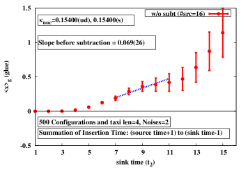
Figure 3: The ratio of three point to two point functions plotted in terms of nucleon sink time $t_{2}$ for quenched configurations with $\kappa=0.1540$. The linear slope corresponds to $\xnuc_{G}$.

4 Strangeness electric and magnetic form factors

We use the point-split vector current as

$$V_{\mu}=\bar{q}(x)(1-\gamma_{\mu})U_{\mu}(x)q(x+\mu)-\bar{q}(x+\mu)(1+\gamma_{\mu})U_{\mu}^{\dagger}(x)q(x).$$ (10)

The advantage of the point-split operator is that there is no additional renormalization factor to be considered, because it is a conserved current. Using this operator, the electric and magnetic form factors can be obtained [3] by the following combination of three point and two point functions:

$$\frac{{\rm Tr}\left[\Gamma_{e}\cdot\Pi^{\rm 3pt}_{V_{\mu=4}}(\vec{0},t_{2};\ \vec{q},t_{1};\ -\vec{q},\vec{x}_{0},t_{0})\right]\times e^{-i\vec{q}\cdot\vec{x}_{0}}}{{\rm Tr}\left[\Gamma_{e}\cdot\Pi^{\rm 2pt}(\vec{q},t_{1};\ \vec{x}_{0},t_{0})\right]\times e^{+i\vec{q}\cdot\vec{x_{0}}}}\cdot\frac{{\rm Tr}\left[\Gamma_{e}\cdot\Pi^{\rm 2pt}(\vec{0},t_{1};\ \vec{x}_{0},t_{0})\right]}{{\rm Tr}\left[\Gamma_{e}\cdot\Pi^{\rm 2pt}(\vec{0},t_{2};\ \vec{x}_{0},t_{0})\right]}$$

$$=\left[F_{1}(-q_{E}^{2})-\frac{E_{q}-m}{2m}F_{2}(-q_{E}^{2})\right]$$ (11)

$$\frac{{\rm Tr}\left[\Gamma_{k}\cdot\Pi^{\rm 3pt}_{V_{\mu=i}}(\vec{0},t_{2};\ \vec{q},t_{1};\ -\vec{q},\vec{x}_{0},t_{0})\right]\times e^{-i\vec{q}\cdot\vec{x}_{0}}}{{\rm Tr}\left[\Gamma_{e}\cdot\Pi^{\rm 2pt}(\vec{q},t_{1};\ \vec{x}_{0},t_{0})\right]\times e^{+i\vec{q}\cdot\vec{x_{0}}}}\cdot\frac{{\rm Tr}\left[\Gamma_{e}\cdot\Pi^{\rm 2pt}(\vec{0},t_{1};\ \vec{x}_{0},t_{0})\right]}{{\rm Tr}\left[\Gamma_{e}\cdot\Pi^{\rm 2pt}(\vec{0},t_{2};\ \vec{x}_{0},t_{0})\right]}$$

$$=(-1)*\frac{1}{E_{q}+m}\epsilon_{ijk}q_{j}^{E}\left(F_{1}(-q_{E}^{2})+F_{2}(-q_{E}^{2})\right),$$ (12)

where $\Gamma_{k}\equiv\left(\begin{array}[]{cc}\sigma_{k}&0\\ 0&0\\ \end{array}\right)$, $m$ denotes nucleon mass, and $E_{q}\equiv\sqrt{m^{2}+\vec{q}^{2}}$.

In Fig. 4, we plot the ratio of three point to two point functions in terms of the nucleon sink time $t_{2}$ where the linear slope corresponds to the signal of strangeness magnetic form factor at $\vec{q}^{2}=(2\pi/L)^{2}$. In order to obtain the final quantitative result for the strangeness magnetic moment, detailed study for several $Q^{2}(-q^{2})$ and chiral extrapolation are needed and they are in progress.

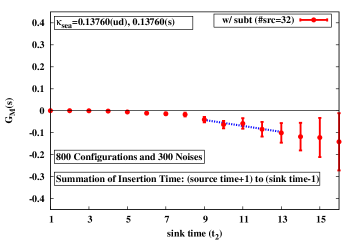
Figure 4: The ratio of three point to two point functions plotted in terms of the nucleon sink time $t_{2}$ for dynamical configurations with $\kappa=0.13760$. The linear slope corresponds to the strangeness magnetic form factor at $\vec{q}^{2}=(2\pi/L)^{2}$

.

5 Summary

We have studied the strangeness and gluonic contribution to the nucleon matrix elements from lattice QCD. The strangeness matrix elements have been studied by the Z(4) stochastic method, with the unbiased subtraction from the hopping parameter expansion in order to reduce the off-diagonal noises. We have further taken many nucleon sources for each configuration, and observed that this method is almost ideally effective to improve the signal with modest cost. Using $N_{f}=2+1$ dynamical clover fermion configurations, we have analyzed the quark contribution to the first moment, $\xnuc_{q}$, and the strangeness magnetic form factor, and found that statistical errors are well under control with these improvements.

The gluonic contribution for the first moment of nucleon, $\xnuc_{G}$, has also been studied with the use of the overlap operator to construct the gauge field tensor, $F_{\mu\nu}$, and we have shown the effectiveness of this method by the explicit calculation at the quenched level.

Although there remain several sources of the systematic error, such as the finite volume artifact, discretization error, excited-states contamination and chiral extrapolation, we plan to investigate these issues by using the configurations with larger volume and lighter quark masses with various lattice cut-offs. The study for other matrix elements such as the angular momentum contribution to the nucleon spin is also in progress.

- [1] J. Ashman et al., An Investigation of the Spin Structure of the Proton in Deep Inelastic Scattering of Polarized Muons on Polarized Protons, Nucl. Phys. B 328 (1989) 1.
- [2] J. Zanotti, Investigations of hadron structure on the lattice, in these proceedings and references therein.
- [3] S.-J. Dong, K.-F. Liu and A. G. Williams, Lattice calculation of the strangeness magnetic moment of the nucleon, Phys. Rev. D 58 (1998) 074504; N. Mathur and S.-J. Dong, Strange magnetic moment of the nucleon from lattice QCD, Nucl. Phys. Proc. Suppl. 94 (2001) 311.
- [4] N. Mathur et al., Quark orbital angular momentum from lattice QCD, Phys. Rev. D 62 (2000) 114504.
- [5] R. Lewis, W. Wilcox and R. M. Woloshyn, The Nucleon’s strange electromagnetic and scalar matrix elements, Phys. Rev. D 67 (2003) 013003.
- [6] D. Mankame et al., 2+1 flavor QCD calculation of and , in these proceedings.
- [7] M. Gockeler et al., A Preliminary lattice study of the glue in the nucleon, Nucl. Phys. Proc. Suppl. 53 (1997) 324.
- [8] K.-F. Liu, A. Alexandru and I. Horvath, Gauge field strength tensor from the overlap Dirac operator, Phys. Lett. B 659 (2008) 773 [hep-lat/0703010].
- [9] T. Ishikawa et al., 2+1 flavor light hadron spectrum and quark masses with the improved Wilson-clover quark formalism, PoS (LAT2006) 181; T. Ishikawa et al., Light quark masses from unquenched lattice QCD, Phys. Rev. D 78 (2008) 011502.
- [10] S.-J. Dong and K.-F. Liu, Stochastic estimation with Z(2) noise, Phys. Lett. B 328 (1994) 130.
- [11] C. Thron, S.-J. Dong, K.-F. Liu and H.P. Ying, Pade - Z(2) estimator of determinants, Phys. Rev. D 57 (1998) 1642.
- [12] X.-D. Ji, Gauge invariant decomposition of nucleon spin and its spin-off, Phys. Rev. Lett. 78 (1997) 610.
- [13] M. Deka et al., Moments of Nucleon’s Parton Distribution for the Sea and Valence Quarks from Lattice QCD, in preparation.