HINODE Observations of Chromospheric Brightenings in the
Ca II H Line during small-scale Flux Emergence Events

Abstract

Ca II H emission is a well-known indicator of magnetic activity in the Sun and other stars. It is also viewed as an important signature of chromospheric heating. However, the Ca II H line has not been used as a diagnostic of magnetic flux emergence from the solar interior. Here we report on Hinode observations of chromospheric Ca II H brightenings associated with a repeated, small-scale flux emergence event. We describe this process and investigate the evolution of the magnetic flux, G-band brightness, and Ca II H intensity in the emerging region. Our results suggest that energy is released in the chromosphere as a consequence of interactions between the emerging flux and the pre-existing magnetic field, in agreement with recent 3D numerical simulations.

1 Introduction

Numerical simulations predict that magnetic flux emerging into the solar atmosphere interact and reconnect with the pre-existing chromospheric and coronal field. This suggests that flux emergence is a relevant source of energy for the chromosphere (Archontis et al., 2004; Archontis et al., 2005). The efficiency of the interaction and the consequent heating seem to depend on the geometry of the two flux systems (Galsgaard et al., 2007). While at large scale these results have been confirmed by high-resolution observations (Moreno-Insertis et al., 2008; Zuccarello et al., 2008), the role of small-scale emergence events in the heating of the upper atmospheric layers, as described by Isobe et al. (2008), is still lacking observational confirmation.

In the absence of other diagnostics, heating events in the chromosphere can be detected through the intensity profiles of the Ca II H and K lines. The correlation between flux emergence and Ca II chromospheric emission was analyzed in detail by Balasubramaniam (2001), who observed anomalous profiles in the K line in an emerging active region. However, very few examples of small-scale transient Ca II brightenings have been reported in the literature, and most of them are related to flux cancellation events (e.g. Bellot Rubio & Beck, 2005).

The Hinode satellite, with its unprecedented spatial resolution, offers for the first time the possibility to investigate the processes that occur in the chromosphere during the emergence of magnetic flux at small spatial scales. In this Letter we analyze simultaneous chromospheric and photospheric observations of an emerging flux region taken with the Solar Optical Telescope aboard Hinode. During the emergence event, strong brightenings were detected in the Ca II H line core without relevant counterparts in G-band intensity, which suggests that chromospheric heating did occur at the site of flux emergence.

2 Observations and data reduction

On 2007 September 30, as part of the Hinode Operation Plan 14 (Hinode/Canary Islands Campaign), the active region NOAA 10971 was observed by the Solar Optical Telescope (SOT; Tsuneta et al., 2008) onboard Hinode (Kosugi et al., 2007). The field of view (FoV) was centered at solar coordinates ($174\arcsec$, $-79\arcsec$), i.e., $11^{\circ}$ away from disk center.

The SOT spectro-polarimeter (SP; Tsuneta et al., 2008) performed six raster scans of the active region from 08:00 to 14:00 UT, acquiring the Stokes I, Q, U, and V profiles of the photospheric Fe I lines at 630.15 nm and 630.25 nm. The FoV covered by the SP observations is $164\arcsec\times 164\arcsec$, with an effective pixel size of $0.32\arcsec$ (Fast Map mode). Simultaneously, the SOT Broadband Filter Imager (BFI) acquired filtergrams in the core of the Ca II H line ($396.85\pm 0.3\;\textrm{nm}$) and in the G band ($430.5\pm 0.8\;\textrm{nm}$), while the Narrowband Filter Imager (NFI) obtained shuttered Stokes I and V filtergrams in the wings of the Na I D1 line at $589.6\;\textrm{nm}$. The BFI images have a spatial sampling of $0.05\arcsec$/pixel (G-band) and $0.1\arcsec$/pixel (Ca II H), while that of the NFI filtergrams is $0.16\arcsec$/pixel. The BFI and NFI time series have a cadence of one minute and extend from 07:00 to 17:00 UT, with a small gap between 10:05 and 10:20 UT.

We have corrected the SOT/SP and SOT/FG images for dark current, flat field, and cosmic rays with standard SolarSoft routines. Besides obtaining photospheric and chromospheric information through corrected G-band and Ca II H filtergrams, we have constructed magnetograms from the Na I D1 Stokes I and V images acquired $\pm 156$ mÅ off the line center. From the ratio

$$\frac{V}{I}=\frac{1}{2}\left(\frac{V_{\rm blue}}{I_{\rm blue}}+\frac{V_{\rm red}}{I_{\rm red}}\right)$$

we calculate the magnetic flux density $\Phi_{\rm d}$ using the weak fied approximation (Stix, 2002) as

$$\Phi_{\rm d}=8\times 10^{3}\>\frac{V}{I}\;\;\;[\textrm{Mx cm}^{-2}]$$

(see Guglielmino, 2008). To first order, the magnetograms computed in this way are not affected by Doppler shifts. We remind the reader that, at disk center, the Na I D1 line refers to the upper photospheric layers and not to the chromosphere.

For each raster scan of the SP, the profile with the minimum total polarization degree, $P=\left[\left(Q^{2}+U^{2}+V^{2}\right)/I^{2}\right]^{1/2}$, was selected as a reference profile. All the spectra in the scan were normalized to the continuum of this profile and corrected for limb darkening. Also, a stray light profile was computed by averaging the reference profiles of the six scans.

Adopting a grid paradigm, we have inverted the spectra with $P>2\%$ using the SIR code (Ruiz Cobo & del Toro Iniesta, 1992). The inversion yields the temperature stratification in the range $-4.0<\log\,\tau_{5}<0$ ($\tau_{5}$ is the optical depth of the continuum at $500\;\textrm{nm}$), together with the magnetic field strength, inclination and azimuth angles in the line-of-sight (los) reference frame, the los velocity, and the magnetic filling factor, assuming these quantities to be constant with height. Azimuth and inclination angles have been transformed to the local solar frame, whereas the los velocity has been calibrated using the mean quiet-Sun intensity profile computed from pixels with $P<0.5\%$, following the procedure of Martínez Pillet et al. (1997).

Finally, all the SOT/FG and SOT/SP images have been aligned through cross-correlation algorithms.

3 Results

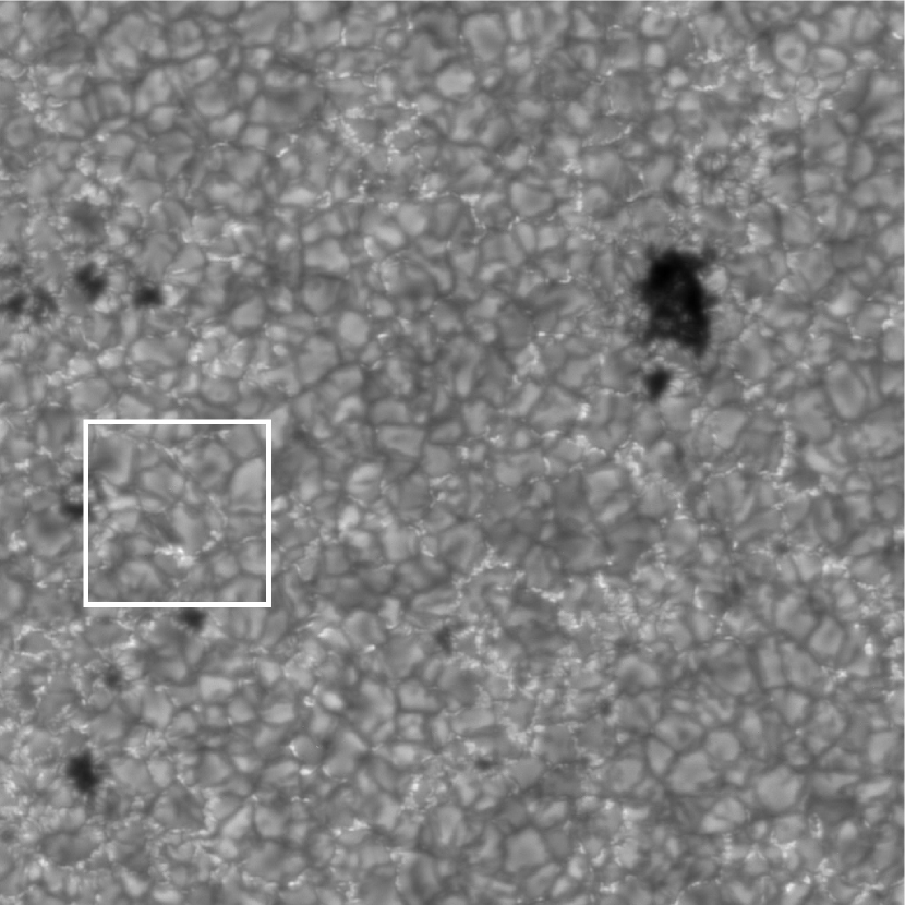
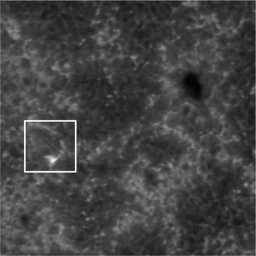
Figure 3: G-band (left) and Ca II H (right) filtergrams (FoV $\sim 80\times 80\;\textrm{Mm}^{2}$) acquired simultaneously at the time of the second peak in Ca II H brightness (12:41 UT). The squares have a FoV of $8\times 8\;\textrm{Mm}^{2}$. They contain a bright structure with a shape similar to that of the emerging region observed with the SOT/SP at 12:23 UT (see Fig. 4).

NOAA 10971 has a classical bipolar $\beta$ configuration, as can be seen in the Na I D1 magnetogram of Fig. 1. The various SOT instruments recorded the emergence of a small bipolar region, which appeared at the internal edge of the main negative polarity. Figure 2 displays a temporal sequence of Na I D1 magnetograms with a cadence of about 20 minutes for the $8\times 8$ Mm² area marked in Fig. 1. The first magnetogram of the sequence, acquired at 07:50 UT, shows the presence of a positive-polarity knot. In the following magnetograms we clearly recognize an increase in its area, as well as the appearance of a negative-polarity patch. The subsequent evolution is characterized by the separation of the opposite magnetic polarities, as indicated by the arrows. The corresponding temporal sequence of Ca II H filtergrams is also displayed in Fig. 2 and shows transient brightness enhancements at the location of the positive footpoint. This emergence event led to the appearance of bright points in the G band (Fig. 3, left panel) and to intensity enhancements in the Ca II H line core (Fig. 3, right panel).

Maps of the physical parameters derived from the SP raster scans are displayed in Fig. 4. They demonstrate the rapid evolution of the small bipolar region: the changes in, e.g., the magnetic field distribution (second and third rows) indicate a very dynamic phase. The small bipolar region shows an emergence zone, i.e., a region between the two main polarities with horizontal fields (Lites et al., 1998) in which upflows of $\sim 1\;\textrm{km s}^{-1}$ can be seen at 9:18 UT and 12:23 UT. The footpoints of the emerging region exhibit vertical fields and downflows of $1.5-2\;\textrm{km s}^{-1}$. The initial photospheric total flux content of the emerging region is $1.4\times 10^{19}\;\textrm{Mx}$, classifying as a small ephemeral region. The bipole axis was inclined about $45\arcdeg$ to the north-south direction in the first raster scan, but this angle varied with time. The negative-polarity footpoint soon merged with the dominant negative flux of the active region, disappearing as an individual feature.

In this area we have detected chromospheric Ca II H brightness enhancements with two main peaks during the observations, each one preceded by a minor peak. As can be seen in Fig. 2, the brightenings are associated with the positive-polarity footpoint. The duration of each peak is about half an hour, with an enhancement of $\sim 80\%$ with respect to the “quiet” level. The presence of these peaks points to interactions between the new emerging and the old pre-existing flux systems. We have computed the average intensity of the four most luminous pixels within the $8\times 8\;\textrm{Mm}^{2}$ FoV for the Ca II H and G-band filtergrams, respectively. Figure 5 shows the trend of brightness in Ca II H and G band in normalized units. The different behaviour indicates that they are not correlated, as the chromospheric brightness enhancements are much more intense than the increase observed in the G band at the same times. Thus, the observed Ca II H enhancements are genuinely due to photons coming from the chromosphere, and not to the significant photospheric contribution included in the passband of the SOT Ca II H filter (Carlsson et al., 2007).

We have calculated the positive flux in the $8\times 8$ Mm² area using the Na I D1 magnetograms, which have a noise level of approximately $6.75\times 10^{14}\;\textrm{Mx/pixel}$. The main contribution to the positive flux comes from the positive polarities of the emerging region. In Fig. 6 we show the flux evolution with time: the chromospheric brightness enhancements clearly correspond to an increase of positive magnetic flux in the upper photosphere. Interestingly, in both cases the maximum Ca II H intensities are reached some 30 minutes after the positive flux starts to increase.

Taking into account the temporal coincidence between the chromospheric brightenings and the positive flux increase, as well as the spatial coincidence between the location and morphology of the Ca II H brightenings and the emerging bipolar region (Fig. 2; compare also the second, third, and fifth rows of Fig. 4), we conclude that the localized chromospheric heating is a consequence of the emergence and subsequent interaction of the positive flux of the new bipole, which cancels with the negative ambient magnetic field.

4 Conclusions

Using Hinode filtergrams and spectropolarimetric measurements, we have studied a small-scale flux emergence event. Two peaks of chromospheric origin have been detected in the Ca II H line-core intensity almost simultaneously to a magnetic flux increase in the upper photosphere.

We suggest that the chromospheric brightness enhancements may be indication that two different flux systems undergo magnetic reconnection: the old flux system belonging to the active region and the emerging magnetic field. The energy released in the process heats the chromosphere. The observed Ca II H brightenings are associated with a relatively modest amount of emerged magnetic flux (only $\sim 4\times 10^{18}\;\textrm{Mx}$ compared with the total negative flux in the region of $\sim 2.5\times 10^{19}\;\textrm{Mx}$), which points to a highly efficient heating mechanism. We conjecture that, while the positive flux increases, part of it cancels with the pre-existing negative flux, very likely in a process of magnetic reconnection.

Our result suggests that Joule dissipation may be a significant source of chromospheric heating during the reconnection of an emerging flux system with a pre-existing magnetic field. This would confirm the predictions of recent numerical simulations (e.g. Galsgaard et al., 2005), also at small scales. Moreover, our work suggests that Ca II H brightness enhancements can be used as a valuable diagnostics of flux emergence. Further investigations should put this result into a firm observational and theoretical basis.

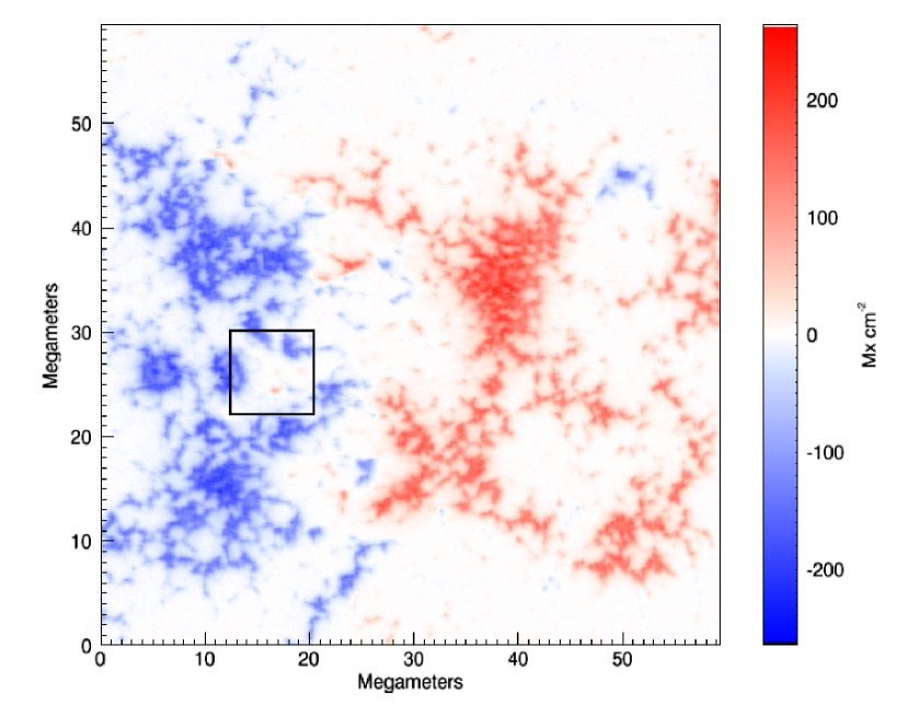
Figure 1: Vertical component of the magnetic field obtained from the Na I magnetograms at 07:50 UT, at the very beginning of the emergence event (FoV $\sim 60\times 60\;\textrm{Mm}^{2}$). The square, with a FoV of $8\times 8\;\textrm{Mm}^{2}$, indicates the location of the emerging flux region analyzed in this Letter.

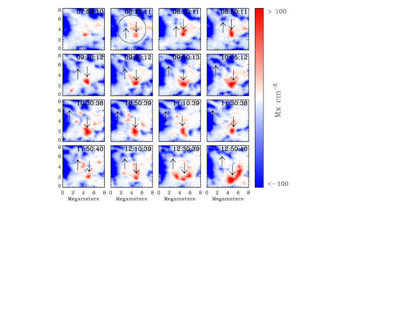
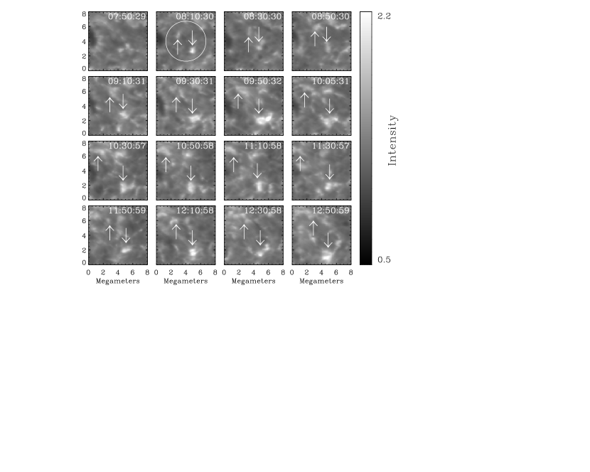
Figure 2: Top: Temporal sequence of Na I D1 magnetograms, starting from 07:50 UT, with a FoV of $8\times 8\;\textrm{Mm}^{2}$. Arrows indicate footpoints of opposite polarity. In the second frame the circle encloses the region highlighted in Fig. 4. Bottom: Same, for the Ca II H filtergrams. Major Ca intensity enhancements are associated with the positive footpoint. Note that the brightening at 09:50 UT occurred above the contact region between the positive flux element of the emerging bipole and the negative ambient magnetic field.

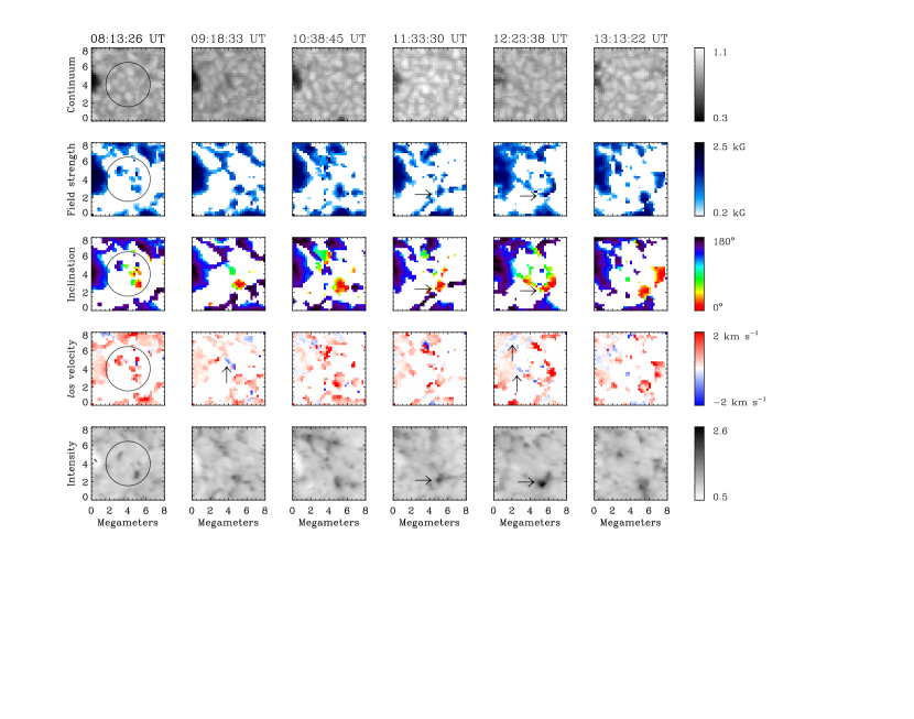
Figure 4: Evolution of physical parameters in the emerging flux region. From top to bottom: continuum intensity, magnetic field strength, inclination, and los velocity, as derived from the inversion of the SOT/SP scans. The FoV is $8\times 8\;\textrm{Mm}^{2}$, corresponding to the squares marked in Fig. 1 and 3. North is up and West to the right. The white background represents non-inverted pixels. The emerging bipolar region is enclosed with a circle in the first scan. In the last row we show Ca II H filtergrams, with reversed color scale. Vertical arrows indicate blueshifts, whereas horizontal arrows indicate the sites of chromospheric brightenings.

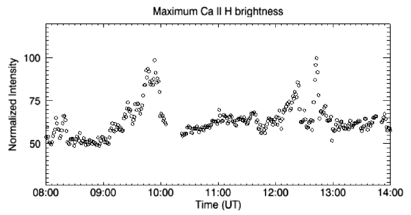
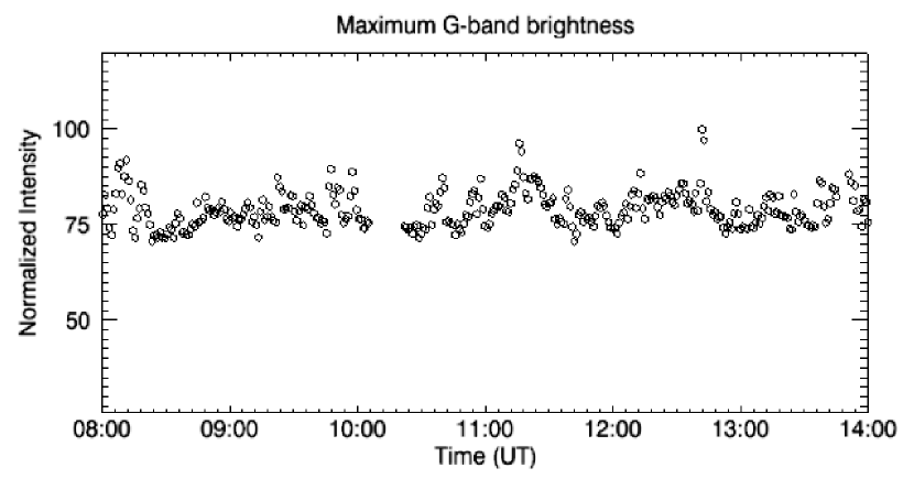
Figure 5: Top: Evolution of the maximum Ca II H brightness (normalized DNs). Two main peaks can be observed at 9:50 UT and 12:40 UT. Bottom: Same, for G-band intensity. The increases are not correlated with Ca II H enhancements.

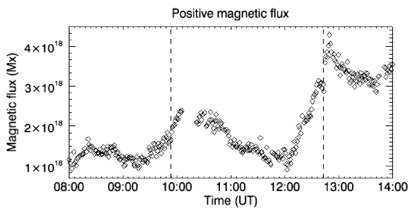
Figure 6: Evolution of the positive magnetic flux in the area, brought by the newly emerging bipole. Uncertainties are of the order of the symbol size. The vertical lines indicate the times of the chromospheric brightenings.

References

- Archontis et al. (2004) Archontis, V., Moreno-Insertis, F., Galsgaard, K., Hood, A., & O’Shea, E. 2004, A&A, 426, 1047
- Archontis et al. (2005) Archontis, V., Moreno-Insertis, F., Galsgaard, K., & Hood, A. W. 2005, ApJ, 635, 1299
- Balasubramaniam (2001) Balasubramaniam, K. S. 2001, ApJ, 557, 366
- Carlsson et al. (2007) Carlsson, M., et al. 2007, PASJ, 59, 663
- Bellot Rubio & Beck (2005) Bellot Rubio, L. R., & Beck, C. 2005, ApJ, 626, L125
- Galsgaard et al. (2005) Galsgaard, K., Moreno-Insertis, F., Archontis, V., & Hood, A. 2005, ApJ, 618, L153
- Galsgaard et al. (2007) Galsgaard, K., Archontis, V., Moreno-Insertis, F., & Hood, A. W. 2007, ApJ, 666, 516
- Guglielmino (2008) Guglielmino, S. L. 2008, Ph.D. Thesis
- Isobe et al. (2008) Isobe, H., Proctor, M. R. E., & Weiss, N. O. 2008, ApJ, 679, L57
- Kosugi et al. (2007) Kosugi, T., et al. 2007, Sol. Phys., 243, 3
- Lites et al. (1998) Lites, B. W., Skumanich, A., & Martínez Pillet, V. 1998, A&A, 333, 1053
- Martínez Pillet et al. (1997) Martínez Pillet, V., Lites, B. W., & Skumanich, A. 1997, ApJ, 474, 810
- Moreno-Insertis et al. (2008) Moreno-Insertis, F., Galsgaard, K., & Ugarte-Urra, I. 2008, ApJ, 673, L211
- Ruiz Cobo & del Toro Iniesta (1992) Ruiz Cobo, B., & del Toro Iniesta, J. C. 1992, ApJ, 398, 375
- Stix (2002) Stix, M. 2002, The Sun: an Introduction (Berlin: Springer)
- Tsuneta et al. (2008) Tsuneta, S., et al. 2008, Sol. Phys., 249, 167
- Zuccarello et al. (2008) Zuccarello, F., Battiato, V., Contarino, L., Guglielmino, S. L., Romano, P., & Spadaro, D. 2008, A&A, 488, 1117