Nonlinear rheological properties of dense colloidal dispersions close to a glass transition under steady shear

The nonlinear rheological properties of dense colloidal suspensions under steady shear are discussed within a first principles approach. It starts from the Smoluchowski equation of interacting Brownian particles in a given shear flow, derives generalized Green-Kubo relations, which contain the transients dynamics formally exactly, and closes the equations using mode coupling approximations. Shear thinning of colloidal fluids and dynamical yielding of colloidal glasses arise from a competition between a slowing down of structural relaxation, because of particle interactions, and enhanced decorrelation of fluctuations, caused by the shear advection of density fluctuations. The integration through transients approach takes account of the dynamic competition, translational invariance enters the concept of wavevector advection, and the mode coupling approximation enables to quantitatively explore the shear-induced suppression of particle caging and the resulting speed-up of the structural relaxation. Extended comparisons with shear stress data in the linear response and in the nonlinear regime measured in model thermo-sensitive core-shell latices are discussed. Additionally, the single particle motion under shear observed by confocal microscopy and in computer simulations is reviewed and analysed theoretically.

Shear modulus of a solid (transverse elastic constant or Lame-coefficient)

Newtonian viscosity of a fluid

Shear stress

Shear rate

Time dependent shear modulus; in the linear response regime denoted as $g^{\rm lr}(t)$ of the quiescent system; generalized one if including dependence on shear rate

Maxwell (final or $\alpha$- relaxation) time of structural relaxation

Storage modulus in linear response

Loss modulus in linear response

Shear viscosity; defined via $\eta=\sigma(\dot{\gamma})/\dot{\gamma}$

Equilibrium structure factor

Hydrodynamic radius of a colloidal particle (radius $a=R_{H}$ assumed)

Colloid diameter ($d=2a=2R_{H}$ assumed throughout)

Thermal energy

Solvent viscosity

Stokes Einstein Sutherland diffusion coefficient at infinite dilution

Bare Peclet number

Dressed Peclet or Weissenberg number

Packing fraction $\phi=\frac{4\pi}{3}R_{H}^{3}n$ of spheres of radius $R_{H}$ at number density $n$

Separation parameter in MCT giving the relative distance in a thermodynamic control parameter to its value at the glass transition

MCT exponent parameter

Instantaneous isothermal shear modulus

High frequency viscosity

Dynamic yield stress of a shear molten glass

Hydrodynamic/ solvent induced interactions

Mode coupling theory

Integrations through transients approach

Smoluchowski operator $\Omega$

Percus-Yevick theory giving the approximate PY $S_{q}$ of a hard sphere fluid

Isotropically sheared hard spheres model

Schematic model without spatial resolution considering a single correlator

1 Introduction

Rheological and elastic properties under flow and deformations are highly characteristic for many soft materials like complex fluids, pastes, sands and gels, viz. soft (often metastable) solids of dissolved macromolecular constituents Larson . Shear deformations, which conserve volume but stretch material elements, often provide the simplest experimental route to investigate the materials. Moreover, solids and fluids respond in a characteristically different way to shear, the former elastically, the latter by flow. The former are characterized by a shear modulus $G_{\infty}$, corresponding to a Hookian spring constant, the latter by a Newtonian viscosity $\eta_{0}$, which quantifies the dissipation.

Viscoelastic materials exhibit both, elastic and dissipative, phenomena depending on external control parameters like temperature and/ or density, and depending on frequency or time-scale of experimental observation. Viscoelastic fluids differ from pastes and sands in the importance of thermal fluctuations causing Brownian motion, which enables them to explore their phase space without external drive like shaking, that would be required to fluidize granular systems. The change between fluid and solid like behavior in viscoelastic materials can have diverse origins, including phase transitions of various kinds, like freezing and micro-phase separation, and/or molecular mechanisms like entanglement formation in polymer melts. One mechanism existent quite universally in dense particulate systems is the glass transition, that structural rearrangements of particles become progressively slower Goe:92 because of interactions/ collisions, and that the structural relaxation time grows dramatically.

Maxwell was the first to describe the viscoelastic response at the fluid-to-glass transition phenomenologically. He introduced a time-dependent shear modulus $g(t)$ describing the response of a viscoelastic fluid to a time-dependent shear deformation,

$$\sigma(t)=\int_{0}^{t}dt^{\prime}\;g(t-t^{\prime})\;\dot{\gamma}(t^{\prime})\;.$$ (1)

Here $\sigma$ is the (transverse) stress, the thermodynamic average of an off-diagonal element of the microscopic stress tensor, and $\dot{\gamma}(t)$ is the time-dependent shear rate impressed on the material starting at time $t=0$. Maxwell chose the Ansatz $g(t)=G_{\infty}\,\exp{\{-(t/\tau)\}}$, which interpolates inbetween elastic behavior $\sigma(t\to 0)\approx G_{\infty}\,\gamma(t)$ for short times $t\ll\tau$ and dissipative behavior, $\sigma(t)\approx\eta_{0}\,\dot{\gamma}(t)$, for long times, $t\gg\tau$; the strain $\gamma(t)$ is obtained from integrating up the strain rate, $\gamma(t)=\int_{0}^{t}dt^{\prime}\dot{\gamma}(t^{\prime})$. Maxwell found the relation $\eta_{0}=G_{\infty}\,\tau$ which connects the structural relaxation time and the glass modulus $G_{\infty}$ to the Newtonian viscosity. He thus explained the increase of the viscosity at the glass transition by the slowing down of the structural dynamics (viz. the increase of $\tau$), and provided a definition of an idealized glass state, where $\tau=\infty$. It responds purely elastically.

Above relation (1) between $\sigma$ and $\dot{\gamma}$ is exact in linear response, where non-linear contributions in $\dot{\gamma}$ are neglected in the stress. The linear response modulus (to be denoted as $g^{\rm lr}(t)$) itself is defined in the quiescent system and describes the small shear-stress fluctuations always present in thermal equilibrium Larson ; russel . Often, oscillatory deformations at fixed frequency $\omega$ are applied and the frequency dependent storage- ($G^{\prime}(\omega)$) and loss- ($G^{\prime\prime}(\omega)$) shear moduli are measured in or out of phase, respectively. The former captures elastic while the latter captures dissipative contributions. Both moduli result from Fourier-transformations of the linear response shear modulus $g^{\rm lr}(t)$, and are thus connected via Kramers-Kronig relations.

The stationary, nonlinear rheological behavior under steady shearing provides additional insight into the physics of dense colloidal dispersions Larson ; russel . Here, the shear rate is constant, $\dot{\gamma}(t)\equiv\dot{\gamma}$, and the stress in the stationary state achieved after waiting sufficiently long (taking $t\to\infty$ in Eq. (1)) is of interest. Equation (1) may be interpreted under flow to state that the non-linearity in the stress versus shear rate curve (the relation $\sigma(\dot{\gamma})$ is termed ’flow curve’) results from the dependence of the (generalized) time-dependent shear modulus $g(t,\dot{\gamma})$ on shear rate. The (often) very strong decrease of the viscosity, defined via $\eta(\dot{\gamma})=\sigma(\dot{\gamma})/\dot{\gamma}$, with increasing flow rate is called ’shear thinning’, and indicates that the particle system is strongly affected by the solvent flow. One may thus wonder whether the particles’ non-affine, random motion relative to the solvent differs qualitatively from the Brownian motion in the quiescent solution. Taylor showed that this is the case for dilute solutions. A single colloidal particle moves super-diffusively at long times along the direction of the flow. Its mean squared non-affine displacement grows with the third power of time, much faster than the linear in time growth familiar from diffusion in the quiescent system . A priori it is thus not clear, whether the mechanisms relevant during glass formation in the quiescent system also dominate the nonlinear rheology. Solvent mediated interactions (hydrodynamic interactions, HI), which do not affect the equilibrium phase diagram, may become crucially important. Also, shear may cause ordering or layering of the particles leading to heterogeneities of various kinds Lau:92 .

Within a number of theoretical approaches a connection between steady state rheology and the glass transition has been suggested. Brady worked out a scaling description of the rheology based on the concept that the structural relaxation arrests at random close packing Bra:93 . In the soft glassy rheology model, the trap model of glassy relaxation by Bouchaud was generalized by Cates and Sollich and coworkers to describe mechanical deformations and ageing Sol:97 ; Sol:98 ; Fie:00 . The mean field approach to spin glasses was generalized to systems with broken detailed balance in order to model flow curves of glasses under shear Ber:00 ; Ber:02 . The application of these novel approaches to colloidal dispersions has lead to numerous insights, but has been hindered by the use of unknown parameters in the approaches.

Dispersions consisting of colloidal, slightly polydisperse (near) hard spheres arguably constitute one of the most simple viscoelastic systems, where a glass transition has been identified. It has been studied in detail by dynamic light scattering measurements Pus:87 ; Meg:91 ; Meg:93 ; Meg:94 ; Meg:98 ; Heb:97 ; Bec:99 ; Bar:02 ; Eck:03 , confocal microscopy Wee:00 , linear Mas:95 ; Zac:06 , and non-linear rheology Sen:99 ; Sen:99b ; Pet:99 ; Pet:02 ; Pet:02b ; Pha:06 ; Bes:07 ; Cra:06 ; Cra:08 ; Sie:09 . Computer simulations are available also Phu:96 ; Str:99 ; Dol:00 . Mode coupling theory (MCT) has provided a semi-quantitative explanation of the observed glass transition phenomena, albeit neglecting ageing effects Pur:06 and decay processes at ultra-long times that may cause (any) colloidal glass to flow ultimately Goe:91 ; Goe:92 ; Goe:99 . It has thus provided a microscopic approach recovering Maxwell’s phenomenological picture of the glass transition; $G_{\infty}$ and $\tau$ could be calculated starting from the particle interactions as functions of the thermodynamic control parameters. MCT was also generalized to include effects of shear on time dependent fluctuations Miy:02 ; miyazaki ; Kob:05 , and, within the integrations through transients (ITT) approach, to quantitatively describe all aspects of stationary states under steady shearing Fuc:02 ; Fuc:05c ; Fuc:09 .

The MCT-ITT approach thus provides a microscopic route to calculate the generalized shear modulus $g(t,\dot{\gamma})$ and other quantities characteristic of the quiescent and the stationary state under shear flow. While MCT has been reviewed thoroughly, see e.g. Goe:91 ; Goe:92 ; Goe:99 , the MCT-ITT approach shall be reviewed here, including its recent tests by experiments in model colloidal dispersions and by computer simulations. The recent developments of microscopy techniques to study the motion of individual particles under flow and the improvements in rheometry and preparation of model systems, provide detailed information to scrutinize the theoretical description, and to discover the molecular origins of viscoelasticity in dense colloidal dispersions even far away from thermal equilibrium.

The outline of the review is as follows: At first, the microscopic starting points, the formally exact manipulations, and the central approximations of MCT-ITT are described in detail. Section 3 summarizes the predictions for the viscoelasticity in the linear response regime and their recent experimental tests. These tests are the quantitatively most stringent ones, because the theory can be evaluated without technical approximations in the linear limit; important parameters are introduced here, also. Section 4 is central to the review, as it discusses the universal scenario of a glass transition under shear. The shear melting of colloidal glasses and the key physical mechanisms behind the structural relaxation in flow are described. Section 5 builds on the insights in the universal aspects and formulates successively simpler models which are amenable to complete quantitative analysis. In the next Section, those models are compared to experimental data on the microscopic particle motion obtained by confocal microscopy, to data on the macroscopic stresses in dispersions of novel model core-shell particles close to equilibrium and under steady flow, and to simulations providing the same information for binary supercooled mixtures. In the last Section, recent generalizations and open questions are addressed.

2 Microscopic approach

MCT considers interacting Brownian particles, predicts a purely kinetic glass transition and describes it using only equilibrium structural input, namely the equilibrium structure factor $S_{q}$ russel ; dhont measuring thermal density fluctuations. MCT-ITT extends this Statistical Mechanics, particle based many-body approach to dispersions in steady flow assuming a linear solvent velocity profile, but neglecting the solvent otherwise.

2.1 Interacting Brownian particles

$N$ spherical particles with radius $R_{H}$ are considered, which are dispersed in a volume $V$ of solvent (viscosity $\eta_{s}$). Homogeneous shear is imposed corresponding to a constant linear solvent velocity profile. The flow velocity points along the $x$-axis and its gradient along the $y$-axis. The motion of the particles (with positions ${\bf r}_{i}(t)$ for $i=1,\ldots,N$) is described by $N$ coupled Langevin equations dhont

$$\zeta\left(\frac{d{\bf r}_{i}}{dt}-{\bf v}^{\rm solv}({\bf r}_{i})\right)={\bf F}_{i}+{\bf f}_{i}\;.$$ (2)

Solvent friction is measured by the Stokes friction coefficient $\zeta=6\pi\eta_{s}R_{H}$. The interparticle forces ${\bf F}_{i}=-\partial/\partial{\bf r}_{i}\,U(\left\{{\bf r}_{j}\right\})$ derive from potential interactions of particle $i$ with all other colloidal particles; $U$ is the total potential energy. The solvent shear-flow is given by ${\bf v}^{\rm solv}({\bf r})=\dot{\gamma}\,y\,\hat{\bf x}$ , and the Gaussian white noise force satisfies (with $\alpha,\beta$ denoting directions)

$$\langle f^{\alpha}_{i}(t)\;f^{\beta}_{j}(t^{\prime})\rangle=2\zeta\,k_{B}T\,\delta_{\alpha\beta}\,\delta_{ij}\,\delta(t-t^{\prime})\;,$$

where $k_{B}T$ is the thermal energy. Each particle experiences interparticle forces, solvent friction, and random kicks from the solvent. Interaction and friction forces on each particle balance on average, so that the particles are at rest in the solvent on average; giving for their affine motion: $\langle{\bf r}_{i}(t)\rangle={\bf r}_{i}(0)+\dot{\gamma}\,t\;y_{i}(0)\,\hat{\bf x}$ . The Stokesian friction is proportional to the particle’s motion relative to the solvent flow at its position; the latter varies linearly along the $y$-direction. The random force on the level of each particle satisfies the fluctuation dissipation relation. The interaction forces ${\bf F}_{i}$ need

Even though Eq. (2) thus has been obtained under the assumption, that solvent fluctuations are close to equilibrium, the Brownian particle system described by it may reach macroscopic states far from thermal equilibrium. Moreover, under (finite) shear, this holds generally because the friction force from the solvent in Eq. (2) can not be derived from a conservative force field. It has non-vanishing curl, and thus the stationary distribution function $\Psi$ describing the probability of the particle positions ${\bf r}_{i}$ can not be of Boltzmann-Gibbs type Risken .

Already the microscopic starting equation (2) of MCT-ITT carries two important approximations. The first is the neglect of hydrodynamic interactions (HI), which would arise from the proper treatment of the solvent flow around moving particles russel ; dhont . As vitrification is observed in molecular systems without HI, MCT-ITT assumes that HI are not central to the glass formation of colloidal dispersions. The interparticle forces are assumed to dominate and to hinder and/or prevent structural rearrangements close to arrest into an amorphous, metastable solid. MCT-ITT assumes that pushing the solvent away only provides some additional instantaneous friction, and thus lets short-time transport properties (like single and collective short-time diffusion coefficients, high frequency viscoelastic response, etc.) depend on HI. The second important approximation in Eq. (2) is the assumption of an homogeneous shear rate $\dot{\gamma}$. This assumption may be considered as a first step, before heterogeneities and confinement effects are taken into account. The interesting phenomena of shear localization and shear banding and shear driven clustering dhontrev ; Ben:96 ; Var:04 ; Gan:06 ; Bal:08 therefore are not addressed. All difficulties in Eq. (2) thus are connected to the many-body interactions given by the forces ${\bf F}_{i}$, which couple the $N$ Langevin equations. In the absence of interactions, ${\bf F}_{i}\equiv 0$, Eq. (2) immediately leads to the super-diffusive particle motion mentioned in the introduction, which often is termed ’Taylor dispersion’ dhont .

As is well known, the considered microscopic Langevin equations, are equivalent to the reformulation of Eq. (2) as Smoluchowski equation; it is a variant of a Fokker-Planck equation Risken . It describes the temporal evolution of the distribution function $\Psi(\left\{{\bf r}_{i}\right\},t)$ of the particle positions

$$\partial_{t}\Psi(\left\{{\bf r}_{i}\right\},t)=\Omega\;\Psi(\left\{{\bf r}_{i}\right\},t)\;,$$ (3a)

employing the Smoluchowski operator (SO) russel ; dhont ,

$$\Omega=\sum_{j=1}^{N}\left[D_{0}\;\frac{\partial}{\partial{\bf r}_{j}}\cdot\left(\frac{\partial}{\partial{\bf r}_{j}}-\frac{1}{k_{B}T}\,{\bf F}_{j}\right)-\dot{\gamma}\,\frac{\partial}{\partial x_{j}}\,y_{j}\right]\;,$$ (3b)

built with the Stokes-Einstein-Sutherland diffusion coefficient $D_{0}=k_{B}T/\zeta$ of a single particle. Averages performed with the distribution function $\Psi$ agree with the ones obtained from the explicit Lagevin equations.

The Smoluchowski equation is a conservation law for the probability distribution in coordinate space,

$$\partial_{t}\,\Psi+\nabla\cdot{\bf j}=\partial_{t}\,\Psi+\sum_{i=1}^{N}\frac{\partial}{\partial{\bf r}_{i}}\cdot{\bf j}_{i}=0\;,$$

formed with probability current $\bf j$. Stationary distributions, which clearly obey $\partial_{t}\,\Psi_{s}=0$, which are not of equilibrium type, are characterised by a non-vanishing probability flux ${\bf j}^{s}_{i}\neq 0$, where

$${\bf j}^{s}_{i}=D_{0}\left[-\frac{\partial}{\partial{\bf r}_{i}}+\frac{1}{k_{B}T}\,{\bf F}_{i}+\dot{\gamma}\,y_{i}\hat{\bf x}\right]\;\Psi_{s}\;.$$

Under shear, ${\bf j}_{s}$ can not vanish, as this would require the gradient term to balance the term proportional to $\dot{\gamma}$ which, however, has a non-vanishing curl; the ’potential conditions’ for an equilibrium stationary state are violated under shear Risken .

The ITT approach formally exactly solves the Smoluchowski equation, following the transients dynamics into the stationary state. In this way the kinetic competition between Brownian motion and shearing, which arises from the stationary flux, is taken into account in the stationary distribution function. To explicitly, but approximatively compute it, using ideas based on MCT, MCT-ITT approximates the obtained averages by following the transient structural changes encoded in the transient density correlator.

2.2 Integration through transients (ITT) approach

2.2.1 Generalized Green-Kubo relations

Formally, the H-theorem valid for general Fokker-Planck equations states that the solution of Eq. (3) becomes unique at long times Risken . Yet, because colloidal particles have a non-penetrable core and exhibit excluded volume interactions, corresponding to regions where the potential is infinite, and the proof of the H-theorem requires fluctuations to overcome all barriers, the formal H-theorem may not hold for non-dilute colloidal dispersions. Nevertheless, we assume that the system relaxes into a unique stationary state at long times, so that $\Psi(t\to\infty)=\Psi_{s}$ holds. This assumption is self-consistent, because later on MCT-ITT finds that under shear all systems are ’ergodic’ and relax into the stationary state. In cases where phase space decomposes into disjoint pockets (’nonmixing dynamics’), the distribution function calculated in Eq. (4) averages over all compartments, and can thus not be used.

As alread stated, homogeneous, amorphous systems are assumed so that the stationary distribution function $\Psi_{s}$ is translationally invariant but anisotropic. The formal solution of the Smoluchowski equation for the time-dependent distribution function

$$\Psi(t)=e^{\Omega\,t}\;\Psi_{e}$$ (4a)

can, by taking a derivative and integrating it up to $$t=\infty$$, be brought into the form Fuc:02 ; Fuc:05c

$$\Psi_{s}=\Psi_{e}+\frac{\dot{\gamma}}{k_{B}T}\;\int_{0}^{\infty}\!\!\!\!dt\;\Psi_{e}\;\sigma_{xy}\;e^{\Omega^{\dagger}t}\;,$$ (4b)

where the adjoint Smoluchowski $\Omega^{\dagger}$ operator arises from partial integrations over the particle positions (anticipating that averages built later on with $\Psi$ are done by integrating out the particle positions). It acts on the quantities to be averaged with $\Psi_{s}$. The assumption of spatial homogeneity rules out the considerations of thermodynamic states where the equilibrium system would e.g. be crystalline. The equilibrium state is described by $\Psi_{e}$, which denotes the equilibrum canonical distribution function, $\Psi_{e}\propto e^{-U/(k_{B}T)}$, which is the time-independent solution of Eq. (3a) for $\dot{\gamma}=0$; in Eq. (4b), it gives the initial distribution at the start of shearing (at $t=0$). The potential part of the stress tensor $\sigma_{xy}=-\sum_{i=1}^{N}F^{x}_{i}\,y_{i}$ entered via $\Omega\Psi_{e}=\dot{\gamma}\,\sigma_{xy}\,\Psi_{e}$. The simple, exact result Eq. (4b) is central to the ITT approach as it connects steady state properties to time integrals formed with the shear-dependent dynamics. Advantageously, the problem to perform steady state averages, denoted by $\langle\ldots\rangle^{(\dot{\gamma})}$, has been simplified to performing equilibrium averages, which will be denoted as $\langle\ldots\rangle$ in the following, and contain the familiar $\Psi_{e}$. The transient dynamics integrated up in the second term of Eq. (4b) contains slow intrinsic particle motion, whose handling is central to the MCT-ITT approach. Generalized Green-Kubo relations, formally valid for arbitrary $\dot{\gamma}$, can be derived from Eq. (4b).

The adjoint Smoluchowski operator was obtained using in the partial integrations over the particle positions the incompressibility condition, ${\rm Trace}\{\boldsymbol{\kappa}\}=0$, which should always holds for the solvents of interest in this review. It takes the explicit form (where boundary contributions are neglected throughout, simplifying the partial integrations):

$$\Omega^{\dagger}=\sum_{i}(\boldsymbol{\partial}_{i}+{\bf F}_{i}+{\bf r}_{i}\cdot\boldsymbol{\kappa}^{T})\cdot\boldsymbol{\partial}_{i}\;.$$

This formula already uses a handy notation employing the shear rate tensor $\boldsymbol{\kappa}=\dot{\gamma}\ \hat{\bf x}\hat{\bf y}$ (that is, $\kappa_{\alpha\beta}=\dot{\gamma}\delta_{\alpha x}\delta_{\beta y}$), and dimensionless quantities. They are introduced by using the particle diameter $d$ as unit of length (throughout we convert $d=2R_{H}$), the combination $d^{2}/D_{0}$ as unit of time, and $k_{B}T$ as unit of energy, whereupon the shear rate turns into the bare Peclet number Pe${}_{0}=\dot{\gamma}d^{2}/D_{0}$. It measures the effect of affine motion with the shear flow compared to the time it takes a single Brownian particle to diffuse its diameter $d$. One of the central questions of the nonlinear rheology of dense dispersions concerns the origin of very strong shear-dependences in the viscoelasticity already for (vanishingly) small bare Pe₀ numbers. Thus we will simplify by assuming Pe${}_{0}\ll 1$, and search for another dimensionless number characterizing the effect of shear.

The formally exact general result for $\Psi_{s}$ in Eq. (4b) can be applied to compute the thermodynamic transverse stress, $\sigma(\dot{\gamma})=\langle\sigma_{xy}\rangle/V$. Equation (4b) leads to an exact non-linear Green-Kubo relation:

$$\sigma(\dot{\gamma})=\dot{\gamma}\int_{0}^{\infty}dt\;g(t,\dot{\gamma})\;,$$ (5a)

where the generalized shear modulus $$g(t,\dot{\gamma})$$ depends on shear rate via the Smoluchowski operator from Eq. (3b)

$$g(t,\dot{\gamma})=\frac{1}{k_{B}TV}\;\langle\,\sigma_{xy}\;e^{\Omega^{\dagger}t}\;\sigma_{xy}\,\rangle^{(\dot{\gamma}=0)}\;.$$ (5b)

This relation is nonlinear in shear rate, because $$\dot{\gamma} \Omega^{\dagger} g(t,\dot{\gamma})$$ appears in the time evolution operator , the adjoint of Eq. (3b). In MCT-ITT, the slow stress fluctuations in will be approximated by following the slow structural rearrangements, encoded in the transient density correlators.

But, before discussing approximations, it’s worthwhile to point out that formally exact explicit expressions for arbitrary steady-state averages can be obtained from Eq. (4b). Using the definition $f(\dot{\gamma})\equiv\langle f_{\bf q=0}\rangle^{(\dot{\gamma})}/V$, where ${\bf q}$ is the wavevector, and $f_{\bf q=0}=\int d{\bf r}f({\bf r})$ denotes the integral over an arbitrary density $f({\bf r})$, one finds the general generalized Green-Kubo relation:

$$f(\dot{\gamma}) = \langle f_{\bf q=0}\rangle/V+\frac{\dot{\gamma}}{V}\;\int_{0}^{\infty}\!\!\!\!\!dt\;\langle\sigma_{xy}\;e^{\Omega^{\dagger}\,t}\;\Delta f_{\bf q=0}\,\rangle\;,$$ (5c)

where the symbol $\Delta X$ for the fluctuation in $X$ was introduced, $\Delta X=X-\langle X\rangle$, because all mean values (which are constants, for these purposes) drop out of the ITT integrals, leaving only the fluctuating parts to contribute. Generalizations of Eq. (5c) valid for structure functions (see e.g. Eq. (6b)) and stationary correlation functions (see Eq. (8)) are presented in Ref. Fuc:05c . Note that all the averages, denoted $\langle\ldots\rangle,$ are evaluated within the (Boltzmann) equilibrium distribution $\Psi_{e}$. Why only ${\bf q}=0$ appears in Eq. (5c) is discussed in Sect. 2.2.2 .

It is these generalized Green-Kubo relations Eq. (5c) which are formally exact even for arbitrary strong flows, and which form the basis for approximations in the MCT-ITT approach. These approximations are guided by the evident aspect that slow dynamics strongly affects the time integral in Eq. (5c). Therefore, in MCT-ITT approximations are employed that aim at capturing the slow structural dynamics close to a glass transition. It would be interesting to employ the generalized Green-Kubo relations also in other contexts, where e.g. entanglements lead to slow dynamics in polymer melts.

2.2.2 Aspects of translational invariance

The generalized Green-Kubo relations contain quantities integrated/ averaged over the whole sample volume. Thus, the aspect of translational invariance/ homogeneity does not become an issue in Eq. (5) yet. A system is translational invariant, if the correlation between two points ${\bf r}$ and ${\bf r}^{\prime}$ depends on the distance ${\bf r}-{\bf r}^{\prime}$ between the two points only. The correlation must not change if both points are shifted by the same amount. (Additionally, any quantity depending on one space point ${\bf r}$ only, must be constant.) A system would be isotropic, if additionally, the correlation only depended on the length of the distance vector, $|{\bf r}-{\bf r}^{\prime}|$; but this obviously can not be expected, because shear flow breaks rotational symmetry of the SO in Eq. (3b). Shear flow also breaks translational symmetry in the SO of Eq. (3b), therefore it is a priori surprising, that translational invariance holds under shear. Moreover, discussion of translational invariance introduces the concept of an advected wavevector, which will become important later on.

The time-dependent distribution function $\Psi(t)$ from Eq. (4a) can be used to show that a translationally invariant equilibrium distribution function $\Psi_{e}$ leads to a translationally invariant steady state distribution $\Psi_{s}$, even though the SO in Eq. (3b) is not translationally invariant itself. To show this, a point in coordinate space $({\bf r}_{1},\ldots,{\bf r}_{N})$ shall be denoted by $\Gamma$, and shall be shifted, $\Gamma\to\Gamma^{\prime}$, with ${\bf r^{\prime}}_{i}={\bf r}_{i}+{\bf a}$ for all $i$; $\bf a$ is an arbitrary constant vector. This gives

$$\Omega^{\dagger}(\Gamma)=\Omega^{\dagger}(\Gamma^{\prime})-{\bf a}\;\boldsymbol{\kappa}^{T}\;{\bf P}\;,\quad\mbox{ with }\,{\bf P}=\sum_{i}\boldsymbol{\partial}_{i}\;,$$

explicitly stating that the SO is not translationally invariant. From Eq. (4a) follows

$$\Psi(\Gamma^{\prime},t)=e^{\Omega(\Gamma)\,t-{\bf P}\,\boldsymbol{\kappa}\,{\bf a}\,t}\;\Psi_{e}(\Gamma)\;,$$

where $\Psi_{e}(\Gamma^{\prime})=\Psi_{e}(\Gamma)$ was used. The SO $\Omega$ and the operator ${\bf P}\,\boldsymbol{\kappa}\,{\bf a}$ commute, because the shear rate tensor satisfies $\boldsymbol{\kappa}\cdot\boldsymbol{\kappa}=0$, and because the sum of all internal forces vanishes due to Newton’s third law:

$$\left({\bf P}\boldsymbol{\kappa}{\bf a}\right)\;\Omega-\Omega\;\left({\bf P}\boldsymbol{\kappa}{\bf a}\right)=$$

$$\sum_{ij}\left\{\left[\boldsymbol{\partial}_{i}(\boldsymbol{\partial}_{j}\cdot\frac{\partial U}{\partial{\bf r}_{j}})-(\boldsymbol{\partial}_{j}\cdot\frac{\partial U}{\partial{\bf r}_{j}})\boldsymbol{\partial}_{i}\right]\boldsymbol{\kappa}{\bf a}-\left[({\bf a}\boldsymbol{\kappa}^{T}\boldsymbol{\partial}_{i})\,({\bf r}_{j}\boldsymbol{\kappa}^{T}\boldsymbol{\partial}_{j})-(\boldsymbol{\partial}_{j}\boldsymbol{\kappa}{\bf r}_{j})(\boldsymbol{\partial}_{i}\boldsymbol{\kappa}{\bf a})\right]\right\}$$

$$=\sum_{j}\left\{\left[\boldsymbol{\partial}_{j}(\cdot\frac{\partial}{\partial{\bf r}_{j}}\left(\sum_{i}\frac{\partial U}{\partial{\bf r}_{i}}\boldsymbol{\kappa}{\bf a}\right))\right]-\left[({\bf a}\boldsymbol{\kappa}^{T}\cdot\boldsymbol{\kappa}^{T}\boldsymbol{\partial}_{j})\right]\right\}=0\;.$$

Therefore, the Baker-Hausdorff theorem vanKampen simplifies Eq. (4a) to

$$\Psi(\Gamma^{\prime},t)=e^{\Omega(\Gamma)\,t}\;e^{-{\bf P}\,\boldsymbol{\kappa}\,{\bf a}\,t}\;\Psi_{e}(\Gamma)=e^{\Omega(\Gamma)\,t}\;e^{-\left(\sum_{i}{\bf F}_{i}\right)\,\boldsymbol{\kappa}\,{\bf a}\,t}\;\Psi_{e}(\Gamma)=e^{\Omega(\Gamma)\,t}\;\Psi_{e}(\Gamma)\;,$$

where the last equality again holds because the sum of all internal forces vanishes. Therefore,

$$\Psi(\Gamma^{\prime},t)=\Psi(\Gamma,t)$$

holds, proving that the time-dependent and consequently the stationary distribution function $\Psi_{s}(\Gamma)=\lim_{t\to\infty}\Psi(\Gamma,t)$ are translationally invariant. This applies, at least, in cases without spontaneous symmetry breaking. Formally, the role of such symmetry breaking is to discard some parts of the steady state distribution function and keep others (with the choice dependent on initial conditions). The distributions developed here discard nothing, and would therefore average over the disjoint symmetry-related states of a symmetry-broken system.

Appreciable simplifications follow from translational invariance for steady-state quantities of wavevector-dependent fluctuations:

$$f_{\bf q}(\Gamma,t)=e^{\Omega^{\dagger}\,t}\;\sum_{i}\;X^{f}_{i}(\Gamma)\;e^{i{\bf q}\cdot{\bf r}_{i}}\;,$$

where e.g. $X^{\varrho}_{i}=1$ describes density fluctuations $\varrho_{\bf q}(t)$, while $X^{\sigma}_{i}=\delta_{\alpha\beta}+(1/2)\sum_{j}^{\prime}(r^{\alpha}_{i}-r^{\alpha}_{j})du(|{\bf r}_{i}-{\bf r}_{j}|)/dr^{\beta}_{i}$ gives the stress tensor element $\sigma_{\alpha\beta}({\bf q})$ for interactions described by the pair-potential $u$. Translational invariance in an infinite sheared system dictates that averages are independent of identical shifts of all particle positions. As the integral over phase space must agree for either integration variables $\Gamma$ or $\Gamma^{\prime}$, steady-state averages can be non-vanishing for zero wavevector only:

$$\frac{1}{V}\;\langle f_{{\bf q}}(t)\rangle^{(\dot{\gamma})}=f_{0}(\dot{\gamma})\;\delta_{\bf q,0}\;.$$

The average density $n=N/V$ and the shear stress $\sigma(\dot{\gamma})=\langle\sigma_{xy}\rangle^{(\dot{\gamma})}/V$ are important examples. Wavevector-dependent steady-state structure functions under shear become anisotropic but remain translationally invariant, so that introduction of a single wavevector suffices. The structure factor built with density fluctuations shall be abbreviated by

$$S_{\bf q}(\dot{\gamma})=\frac{1}{N}\;\langle\delta\varrho^{*}_{\bf q}\;\delta\varrho_{\bf q}\rangle^{(\dot{\gamma})}\;.$$ (6a)

It needs to be kept apart from the equilibrium structure factor, denoted by

$$S_{q}=\frac{1}{N}\;\langle\delta\varrho^{*}_{\bf q}\;\delta\varrho_{\bf q}\rangle\;,$$ (6b)

which is obtained by averaging over the particle positions using the equilibrium distribution function $\Psi_{e}$. It will be one of the hallmarks of a shear molten, yielding glass state, that even in the limit of vanishing shear rate both structure factors do not agree: $S_{\bf q}(\dot{\gamma}\to 0)\neq S_{q}$ in a shear molten glassy state.

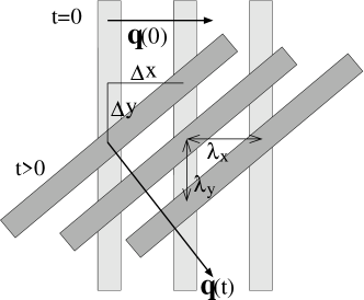
Figure 1: Shear advection of a fluctuation with initial wavevector in $x$-direction, ${\bf q}(t\!\!=\!\!0)=q\,(1,0,0)^{T}$, and advected wavevector at later time ${\bf q}(t\!\!>\!\!0)=q\,(1,-\dot{\gamma}t,0)^{T}$; from Fuc:09 . While $\lambda_{x}$ is the wavelength in $x$-direction at $t=0$, at later time $t$, the corresponding wavelength $\lambda_{y}$ in (negative) $y$-direction obeys: $\lambda_{x}/\lambda_{y}=\Delta x/\Delta y=\dot{\gamma}t$. At all times, ${\bf q}(t)$ is perpendicular to the planes of constant fluctuation amplitude. Note that the magnitude $q(t)=q\sqrt{1+(\dot{\gamma}t)^{2}}$ increases with time. Brownian motion, neglected in this sketch, would smear out the fluctuation.

Translational invariance of sheared systems takes a special form for two-time correlation functions, because a shift of the point in coordinate space from $\Gamma$ to $\Gamma^{\prime}$ gives

$$\langle\delta f^{*}_{{\bf q}}\;e^{\Omega^{\dagger}\,t}\,\delta g_{{\bf k}}\rangle^{(\dot{\gamma})}=e^{-i\left({\bf k}\cdot\boldsymbol{\kappa}\,t+{\bf k}-{\bf q}\right)\cdot\bf{a}}\;\langle\delta f^{*}_{{\bf q}}\;e^{\Omega^{\dagger}\,t}\,\delta g_{{\bf k}}\rangle^{(\dot{\gamma})}\;,$$

while obviously both averages need to agree. Therefore, a fluctuation with wavevector $\bf q$ is correlated with a fluctuation of ${\bf k}={\bf q}(t)$ with the advected wavevector

$${\bf q}(t)={\bf q}-{\bf q}\cdot\boldsymbol{\kappa}\,t$$ (7)

at the later time $t$; only then the exponential in the last equation becomes unity; fluctuations with other wavevector combinations are decorrelated. The advected wavevector’s $y$-component decreases with time as $q_{y}(t)=q_{y}-\dot{\gamma}\,t\;q_{x}$, corresponding to an (asymptotically) decreasing wavelength, which the shear-advected fluctuation exhibits along the $y$-direction; see Fig. 1. Taking into account this time-dependence of the wavelength of fluctuations, a stationary time-dependent correlation function characterized by a single wavevector can be defined:

$$C_{fg;{\bf q}}(t)=\frac{1}{N}\,\langle\delta f^{*}_{{\bf q}}\;e^{\Omega^{\dagger}\,t}\,\delta g_{{\bf q}(t)}\rangle^{(\dot{\gamma})}\;.$$ (8)

Application of Eqs. (4,5) is potentially obstructed by the existence of conservation laws, which may cause a zero eigenvalue of the (adjoint) SO, $\Omega^{\dagger}$. The time integration in Eqs. (4b,5) would then not converge at long times. This possible obstacle when performing memory function integrals, and how to overcome it, is familiar from equilibrium Green-Kubo relations Forster75 . For Brownian particles, only the density $\varrho$ is conserved. Yet, density fluctuations do not couple in linear order to the shear-induced change of the distribution function Fuc:05c . The (equilibrium) average

$$\langle\sigma_{xy}\,e^{\Omega^{\dagger}t}\,\varrho_{\bf q}\rangle=0$$

vanishes for all ${\bf q}$; at finite ${\bf q}$ because of translational invariance, and at ${\bf q}=0$ because of inversion symmetry. Thus, the projector $Q$ can be introduced

$$Q=1-P\;,\quad\mbox{with }\;P=\sum_{\bf q}\delta\varrho_{\bf q}\,\rangle\;\frac{1}{NS_{q}}\;\langle\,\delta\varrho^{*}_{\bf q}\;.$$ (9)

It projects any variable into the space perpendicular to linear density fluctuations. Introducing it into Eq. (5c) is straight forward, because couplings to linear density can not arise in it anyway. One obtains

$$f(\dot{\gamma}) = \langle f_{\bf q=0}\rangle/V+\frac{\dot{\gamma}}{V}\;\int_{0}^{\infty}\!\!\!\!\!dt\;\langle\sigma_{xy}\,Q\;e^{Q\,\Omega^{\dagger}\,Q\,t}\;Q\,\Delta f_{\bf q=0}\,\rangle\;,$$ (5d)

The projection step is exact, and also formally redundant at this stage; but it will prove useful later on, when approximations are performed.

2.2.3 Coupling to structural relaxation

The generalized Green-Kubo relations, leave us with the problem of how to approximate time-dependent correlation functions in Eq. (5). Their physical meaning is that at time zero, an equilibrium stress fluctuation arises; the system then evolves under internal and shear-driven motion until time $t$, when its correlation with a fluctuation $\Delta f_{\bf q=0}$ is determined. Integrating up these contributions for all times since the start of shearing gives the difference of the shear-dependent quantities to the equilibrium ones. During the considered time evolution, the projector $Q$ prevents linear couplings to the conserved particle density.

The time dependence and magnitudes of the correlations in Eq. (5) shall now be approximated by using the overlaps of both the stress and $\Delta f_{\bf q=0}$ fluctuations with appropriately chosen ‘relevant slow fluctuations’. For the dense colloidal dispersions of interest, the relevant structural rearrangements are assumed to be density fluctuations. Because of the projector $Q$ in Eq. (5d), the lowest nonzero order in fluctuation amplitudes, which we presume dominant, must then involve pair-products of density fluctuations, $\varrho_{\bf k}\,\varrho_{\bf p}$.

The mode coupling approximation may be summarized as a rule that applies to all fluctuation products that exhibit slow structural relaxations but whose variables cannot couple linearly to the density. Their time-dependence is approximated as:

$$Q\;e^{Q\Omega^{\dagger}Qt}\;Q\approx\sum_{{\bf k}>{\bf p}}\;Q\,\varrho_{{{\bf k}(-t)}}\,\varrho_{{{\bf p}(-t)}}\;\rangle\;\frac{\Phi_{{\bf k}(-t)}(t)\;\Phi_{{\bf p}(-t)}(t)}{N^{2}S_{{k}}\,S_{{p}}}\;\langle\;\varrho^{*}_{{\bf k}}\,\varrho^{*}_{{\bf p}}\,Q$$ (10a)

The fluctuating variables are thereby projected onto pair-density fluctuations, whose time-dependence follows from that of the transient density correlators $$\Phi_{{\bf q}(t)}(t) Q$$, defined in Eq. (12) below. These describe the relaxation (caused by shear, interactions and Brownian motion) of density fluctuations with equilibrium amplitudes. Higher order density averages are factorized into products of these correlators, and the reduced dynamics containing the projector is replaced by the full dynamics. The entire procedure is written in terms of equilibrium averages, which can then be used to compute nonequilibrium steady states via the ITT procedure. The normalization in Eq. (10a) is given by the equilibrium structure factors such that the pair density correlator with reduced dynamics, which does not couple linearly to density fluctuations, becomes approximated to:

$$\langle\,\varrho^{*}_{{\bf k}}\,\varrho^{*}_{{\bf p}}\,Q\;e^{Q\Omega^{\dagger}Qt}\;Q\,\varrho_{{{\bf k}(t)}}\,\varrho_{{{\bf p}(t)}}\,\rangle\approx N^{2}S_{k}\,S_{p}\;\Phi_{{\bf k}}(t)\;\Phi_{{\bf p}}(t)\;.$$ (10b)

This equation can be considered as central approximation of the MCT Goe:91 and MCT-ITT approach. While the projection onto density pairs, which is also contained/implied in Eq. (10a) may be improved upon systematically by including higher order density or other fluctuations, see schofield ; Goe:87 for examples, no systematic way to improve upon the breaking of averages in Eq. (10b) has been discovered up to now, to the knowledge of the author.

The mode coupling approximations introduced above can now be applied to the exact generalized Green-Kubo relations Eq. (5d). Steady state expectation values are approximated by projection onto pair density modes, giving

$$f(\dot{\gamma})\approx\langle f_{\bf 0}\rangle/V+\frac{\dot{\gamma}}{2V}\int_{0}^{\infty}\!\!\!dt\;\sum_{{\bf k}}\frac{k_{x}k_{y}(-t)S^{\prime}_{k(-t)}}{k(-t)\;S^{2}_{k}}\;V^{f}_{{\bf k}}\;\Phi^{2}_{{\bf k}(-t)}(t)\,\;,$$ (11a)

with $$t \Phi^{*}_{\bf k}=\Phi_{-{\bf k}}=\Phi_{{\bf k}} {\bf k}>{\bf p} \frac{1}{2} {\bf k}$$ the time since switch-on of shear. To derive this, the property was used; also the restriction when summing over wavevectors was dropped, and a factor introduced, in order to have unrestricted sums over . Within Eq. (11a) we have already substituted the following explicit result for the equal-time correlator of the shear stress with density products:

$$\langle\sigma_{xy}\;Q\;\varrho_{{\bf k}(-t)}\;\varrho_{{\bf p}(-t)}\rangle=N\frac{k_{x}\,k_{y}(-t)}{k(-t)}\;S^{\prime}_{k(-t)}\;\delta_{{\bf k}(-t),-{\bf p}(-t)}=\frac{N}{\dot{\gamma}}\;\partial_{t}S_{q(-t)}\;\delta_{{\bf k},-{\bf p}}\;.$$ (11b)

It’s an exact equality using the equilibrium distribution function and Eq.(6)

$$\langle\sigma_{xy}\;Q\;\varrho_{{\bf k}}\;\varrho^{*}_{{\bf k}}\rangle=\langle\sigma_{xy}\;\varrho_{{\bf k}}\;\varrho^{*}_{{\bf k}}\rangle=\int d\Gamma\Psi_{e}(-\sum_{i}F^{x}_{i}y_{i})\;\varrho_{{\bf k}}\;\varrho^{*}_{{\bf k}}$$

$$=\int d\Gamma\Psi_{e}(\sum_{i}\partial^{x}_{i}y_{i})\;\varrho_{{\bf k}}\;\varrho^{*}_{{\bf k}}=ik_{x}\sum_{ij}\langle y_{i}(e^{i{\bf k}({\bf r}_{i}-{\bf r}_{j})}-e^{-i{\bf k}({\bf r}_{i}-{\bf r}_{j})})\rangle$$

Equation (11a), as derived via the mode-coupling rule detailed above, contains a ‘vertex function’ $V^{f}_{{\bf k}}$, describing the coupling of the desired variable $f$ to density pairs. This denotes the following quantity, computed using familiar thermodynamic equalities

$$V^{f}_{{\bf k}}\equiv\langle\varrho_{{\bf k}}^{*}\varrho_{{\bf k}}\;Q\;\Delta f_{\bf 0}\rangle/N=\langle\varrho_{{\bf k}}^{*}\varrho_{{\bf k}}\;\Delta f_{\bf 0}\rangle/N-S_{0}\left(S_{k}+n\,\frac{\partial S_{k}}{\partial n}\right)\frac{1}{V}\left.\frac{\partial\langle f_{\bf 0}\rangle}{\partial n}\right)_{T}\;.$$ (11c)

In ITT, the slow stress fluctuations in $g(t,\dot{\gamma})$ are approximated by following the slow structural rearrangements, encoded in the transient density correlators. The generalized modulus becomes, using the approximation Eq. (10a) and the vertex Eq. (11b):

$$g(t,\dot{\gamma})=\frac{k_{B}T}{2}\,\int\!\!\frac{d^{3}k}{(2\pi)^{3}}\;\frac{k_{x}^{2}k_{y}k_{y}(-t)}{k\,k(-t)}\;\frac{S^{\prime}_{k}S^{\prime}_{k(-t)}}{S^{2}_{k}}\;\Phi^{2}_{{\bf k}(-t)}(t)\;,$$ (11d)

Summation over wavevectors has been turned into integration in Eq. (11d) considering an infinite system.

The familiar shear modulus of linear response theory describes thermodynamic stress fluctuations in equilibrium, and is obtained from Eqs. (5b,11d) by setting $\dot{\gamma}=0$ Larson ; russel ; Nae:98 . While Eq. (5b) then gives the exact Green-Kubo relation, the approximation Eq. (11d) turns into the well-studied MCT formula (see Eq. (17) below). For finite shear rates, Eq. (11d) describes how affine particle motion causes stress fluctuations to explore shorter and shorter length scales. There the effective forces, as measured by the gradient of the direct correlation function, $S^{\prime}_{k}/S_{k}^{2}=nc^{\prime}_{k}=n\partial c_{k}/\partial k$, become smaller, and vanish asympotically, $c^{\prime}_{k\to\infty}\to 0$; the direct correlation function $c_{k}$ is connected to the structure factor via the Ornstein-Zernicke equation $S_{k}=1/(1-n\,c_{k})$, where $n=N/V$ is the particle density. Note, that the equilibrium structure suffices to quantify the effective interactions, while shear just pushes the fluctuations around on the ’equilibrium energy landscape’.

While, in the linear response regime, modulus and density correlator are measurable quantities, outside the linear regime, both quantities serve as tools in the ITT approach only. The transient correlator and shear modulus provide a route to the stationary averages, because they describe the decay of equilibrium fluctuations under external shear, and their time integral provides an approximation for the stationary distribution function. Determination of the frequency dependent moduli under large amplitude oscillatory shear has become possible recently only Miy:06 , and requires an extension of the present approach to time dependent shear rates in Eq. (3) Bra:07 .

2.2.4 Transient density correlator

In ITT, the evolution towards the stationary distribution at infinite times is approximated by following the slow structural rearrangements, encoded in the transient density correlator $\Phi_{\bf q}(t)$. It is defined by Fuc:02 ; Fuc:05c

$$\Phi_{\bf q}(t)=\frac{1}{NS_{q}}\;\langle\,\delta\varrho^{*}_{{\bf q}}\;e^{\Omega^{\dagger}t}\;\delta\varrho_{{\bf q}(t)}\,\rangle^{(\dot{\gamma}=0)}\;.$$ (12)

It describes the fate of an equilibrium density fluctuation with wavevector ${\bf q}$, where $\varrho_{\bf q}=\sum_{j=1}^{N}e^{i{\bf q}\cdot{\bf r}_{j}}$, under the combined effect of internal forces, Brownian motion and shearing. Note that because of the appearance of $\Psi_{e}$ in Eq. (4), the average in Eq. (12) can be evaluated with the equilibrium canonical distribution function, while the dynamical evolution contains Brownian motion and shear advection. The normalization is given by $S_{q}$ the equilibrium structure factor russel ; dhont for wavevector modulus $q=|{\bf q}|$. The advected wavevector from Eq. (7) enters in Eq. (12). The time-dependence in ${\bf q}(t)$ results from the affine particle motion with the shear flow of the solvent. Again, irrespective of the use of $\Psi_{e}$ in Eq. (12), or $\Psi_{s}$ in Eq. (8), in both cases translational invariance under shear dictates that at a time $t$ later, the density fluctuation $\delta\varrho^{*}_{\bf q}$ has a nonvanishing overlap only with the advected fluctuation $\delta\varrho_{{\bf q}(t)}$. Figure 1 again applies, where a non-decorrelating fluctuation is sketched under shear. In the case of vanishing Brownian motion, viz. $D_{0}=0$ in Eq. (3b), we find $\Phi_{{\bf q}}(t)\equiv 1$, because the advected wavevector takes account of simple affine particle motion. The relaxation of $\Phi_{{\bf q}}(t)$ thus heralds decay of structural correlations by Brownian motion, affected by shear.

2.2.5 Zwanzig-Mori equations of motion

Structural rearrangements of the dispersion affected by Brownian motion is encoded in the transient density correlator. Shear induced affine motion, viz.  the case $D_{0}=0$, is not sufficient to cause $\Phi_{\bf k}(t)$ to decay. Brownian motion of the quiescent correlator $\Phi^{(\dot{\gamma}=0)}_{k}(t)$ leads at high densities to a slow structural process which arrests at long times in (metastable) glass states. Thus the combination of structural relaxation and shear is interesting. The interplay between intrinsic structural motion and shearing in $\Phi_{\bf k}(t)$ is captured by $(i)$ first a formally exact Zwanzig-Mori type equation of motion, and $(ii)$ second a mode coupling factorisation in the memory function built with longitudinal stress fluctuations Fuc:02 ; Fuc:05c ; Fuc:09 . The equation of motion for the transient density correlators is

$$\partial_{t}\Phi_{\bf q}(t)+\Gamma_{\bf q}(t)\;\left\{\Phi_{\bf q}(t)+\int_{0}^{t}dt^{\prime}\;m_{\bf q}(t,t^{\prime})\;\partial_{t^{\prime}}\,\Phi_{\bf q}(t^{\prime})\right\}=0\;,$$ (13)

where the initial decay rate $\Gamma_{\bf q}(t)=D_{0}\,q^{2}(t)/S_{q(t)}$ generalizes the familiar result from linear response theory to advected wavevectors; it contains Taylor dispersion mentioned in the introduction, and describes the short time behavior, $\Phi_{{\bf q}}(t\to 0)\to 1-\Gamma_{{\bf q}}(0)\,t+\ldots$ .

2.2.6 Mode-coupling closure

The memory equation contains fluctuating stresses and similarly like $g(t,\dot{\gamma})$ in Eq. (11d), is calculated in mode coupling approximation using Eq. (10a) giving:

$$m_{\bf q}(t,t^{\prime})=\frac{1}{2N}\sum_{{\bf k}}V_{{\bf q}{\bf k}{\bf p}}(t,t^{\prime})\;\Phi_{{\bf k}(t^{\prime})}(t-t^{\prime})\;\Phi_{{\bf p}(t^{\prime})}(t-t^{\prime})\;,$$ (14a)

where we abbreviated $${\bf p}={\bf q}-{\bf k}$$. The vertex generalizes the expression in the quiescent case, see Eq. (18c) below, and depends on two times capturing that shearing decorrelates stress fluctuations Fuc:02 ; Fuc:05c ; Fuc:09

$$V_{{\bf q}{\bf k}{\bf p}}(t,t^{\prime}) = \frac{S_{{\bf q}(t)}\,S_{{\bf k}(t^{\prime})}\,S_{{\bf p}(t^{\prime})}}{q^{2}(t)\,q^{2}(t^{\prime})}\;{\cal V}_{{\bf q}{\bf k}{\bf p}}(t)\;{\cal V}_{{\bf q}{\bf k}{\bf p}}(t^{\prime})\,,$$

$${\cal V}_{{\bf q}{\bf k}{\bf p}}(t) = {\bf q}(t)\cdot\left(\,{\bf k}(t)\;nc_{k(t)}+{\bf p}(t)\;nc_{p(t)}\,\right)\;.$$ (14b)

With shear, wavevectors in Eq. (14) are advected according to Eq. (7).

The summarized MCT-ITT equations form a closed set of equations determining rheological properties of a sheared dispersion from equilibrium structural input Fuc:02 ; Fuc:05c ; Fuc:09 . Only the static structure factor $S_{q}$ is required to predict $(i)$ the time dependent shear modulus within linear response, $g^{\rm lr}(t)=g(t,\dot{\gamma}=0)$, and $(ii)$ the stationary stress $\sigma(\dot{\gamma})$ from Eq. (5a).

2.3 A microscopic model: Brownian hard spheres

In the microscopic ITT approach, the rheology is determined from the equilibrium structure factor $S_{q}$ alone. This holds at low enough frequencies and shear rates, and excludes a single time scale, to be denoted by the parameter $t_{0}$ in Eq. (22b), which needs to be found by matching to the short time dynamics. This prediction has as consequence that the moduli and flow curves should be a function only of the thermodynamic parameters characterizing the present system, viz. its structure factor. Because the structure factor for simple fluids far away from demixing and other phase separation regions can be mapped onto the one of hard spheres, the system of hard spheres plays a special role in the MCT-ITT approach. It provides the most simple microscopic model where slow strucutral dynamics can be studied. Moreover, other experimental systems can be mapped onto it by chosing an effective packing fraction $\phi_{\rm eff}=(4\pi/3)nR_{H}^{3}$ and particle radius so that the structure factors agree.

The claim that the rheology follows from $S_{q}$ is supported if the rheological properties of a dispersion only depend on the effective packing fraction, if particle size is taken account of properly. Obviously, appropriate scales for frequency, shear rate and stress magnitudes need to be chosen to observe this; see Sect. 6.2. The dependence of the rheology (via the vertices) on $S_{q}$ suggests that $k_{B}T$ sets the energy scale as long as repulsive interactions dominate the local packing. The length scale is set by the average particle separation, which can be taken to scale with $R_{H}$. The time scale of the glassy rheology within ITT is given by $t_{0}$, which should scale with the measured dilute diffusion coefficient $D_{0}$. Thus the rescaling of the rheological data can be done with measured parameters alone.

Because the hard sphere system thus provides the most simple system to test and explore MCT-ITT, numerical calculations only for this model will be reviewed in the present overview. Input for the structure factor is required, which, for simplicity, will be taken from the analytical Percus-Yervick (PY) approximation russel ; Goe:92 . Straightforward discretization of the wavevector integrals will be performed as discussed below, and in detail in the quoted original papers.

2.4 Accounting for hydrodynamic interactions

Solvent-particle interactions (viz. the HI) act instantaneously if the particle microstructure differs from the equilibrium one, but do not themselves determine the equilibrium structure dhont ; russel . If one assumes that glassy arrest is connected with the ability of the system to explore its configuration space and to approach its equilibrium structure, then it appears natural to assume that the solvent particle interactions are characterized by a finite time scale $\tau_{\rm HI}$. And that they do not shift the glass transition nor affect the frozen glassy structure. HI would thus only lead to an increase of the high frequency viscosity above the solvent value; this value shall be denoted as $\eta_{\infty}$:

$$g(t,\dot{\gamma})\to g(t,\dot{\gamma})+\eta_{\infty}\delta(t-O+)\;.$$ (15a)

The parameter $$\eta_{\infty}$$ would thus characterize a short-time, high frequency viscosity and model viscous processes which require no structural relaxation. It can be measured from the high frequency dissipation

$$G^{\prime\prime}(\omega\to\infty)=\eta_{\infty}\;\omega\;.$$ (15b)

For identical reasoning, also the short time diffusion in the collective (and single particle) motion will be affected by HI. The most simple approximation is to adjust the initial decay rate

$$\Gamma_{\bf q}(t)=D_{s}\,q^{2}(t)/S_{q(t)}\;,$$ (15c)

where the collective short time diffusion coefficient $$D_{s}$$ accounts for HI and other (almost) instantaneous effects which affect the short time motion, and which are not explicitly included in the MCT-ITT approach.

The naive picture sketched here, is not correct for a number of reasons. It is well known that for hard spheres without HI the quiescent shear modulus diverges for short times, $g^{\rm lr,HSnoHI}(t\to 0)\sim t^{-1/2}$. Lubrication forces, which keep the particles apart, eliminate this divergence and render $g^{\rm lr,HI}(t\to 0)$ finite Lio:94 . Thus, the simple separation of the modulus into HI and potential part is not possible for short times, at least for particles with a hard core. Moreover, comparison of simulations without and with HI has shown that the increase of $(\eta_{0}-\eta_{\infty})/\eta_{\infty}$ depends somewhat on HI, and thus not just on the potential interactions as implied.

Nevertheless the sketched picture provides the most basic view of a glass transition in colloidal suspensions, connecting it with the increase of the structural relaxation time $\tau$. Increased density or interactions cause a slowing down of particle rearrangements which leave the HI relatively unaffected, as these solvent mediated forces act on all time scales. Potential forces dominate the slowest particle rearrangements because vitrification corresponds to the limit where they actually prevent the final relaxation of the microstructure. The structural relaxation time $\tau$ diverges at the glass transition, while $\tau^{\rm HI}$ stays finite. Thus close to arrest a time scale separation is possible, $\tau\gg\tau^{{\rm HI}}$.

2.5 Comparison with other MCT inspired approaches to sheared fluids

The MCT-ITT approach aims at describing the steady state properties of a concentrated dispersion under shear. Stationary averages are its major output, obtained via the integration through transients procedure from (approximate) transient fluctuation functions, whose strength is the equilibrium one, and whose dynamics originates from the competition between Brownian motion and shear induced decorrelation. In this respect, the MCT-ITT approach differs from the interesting recent generalization of MCT to sheared systems by Miyazaki, Reichman and coworkers Miy:02 ; miyazaki . These authors considered the stationary but time-dependent fluctuations around the steady state, whose amplitude is the stationary correlation function, e.g. in the case of density fluctuations, it is the distorted structure factor $S_{\bf q}(\dot{\gamma})$ Eq. (6a). In the approach by Miyazaki et al. this structure factor is an input-quantity required to calculate the dynamics, while it is an output quantity, calculated in MCT-ITT from the equilibrium $S_{q}$ of Eq. (6b). Likewise, the stationary stress as function of shear rate, viz. the flow curve $\sigma(\dot{\gamma})$, is a quantity calculated in MCT-ITT, albeit using mode coupling approximations, while in the approach of Refs. Miy:02 ; miyazaki additional ad-hoc approximations beyond the mode coupling approximation are required to access $\sigma(\dot{\gamma})$. Thus, while the scenario of an non-equilibrium transition between a shear-thinning fluid and a shear molten glass, characterized by universal aspects in e.g. $\sigma(\dot{\gamma})$ — see the discussion in Sect. 4 — forms the core of the MCT-ITT results, this scenario can not be directly addressed based on Refs. Miy:02 ; miyazaki .

Because the recent experiments and simulations reviewed here concentrated on the universal aspects of the novel non-equilibrium transition, focus will be laid on the MCT-ITT approach. Reassuringly, however, many similarities between the MCT-ITT equations and the results by Miyazaki and Reichman exist, even though these authors used a different, field theoretic approach to derive their results. This supports the robustness of the mechanism of shear-advection in Eq. (7) entering the MCT vertices in Eqs. (11d,14), which were derived independently in Refs. Miy:02 ; miyazaki and Refs. Fuc:02 ; Fuc:05c ; Fuc:09 from quite different theoretical routes. This mechanism had been known from earlier work on the dynamics of critical fluctuations in sheared systems close to phase transition points Onu:79 , on current fluctuations in simple liquids Kaw:73 , and on incoherent density fluctuations in dilute solutions Ind:95 . Different possibilities also exist to include shear into MCT-inspired approaches, especially the one worked out by Schweizer and coworkers including strain into an effective free energy Kob:05 . This approach does not recover the (idealized) MCT results reviewed below but starts from the extended MCT where no true glass transition exists and describes a crossover scenario without e.g. a true dynamic yield stress as discussed below.

3 Microscopic results in linear response regime

Before turning to the properties of the stationary non-equilibrium states under shear, it is useful to investigate the quiescent dispersion close to vitrification. Consensus on the ultimate mechanism causing glassy arrest may yet be absent, yet, the so-called ’cage effect’ has lead to a number of fruitful insights into glass formation in dense colloidal dispersions. For example, it was extended to particles with a short ranged attraction leading to at first surprising predictions sciortino ; bergen ; dawson ; pham1 .

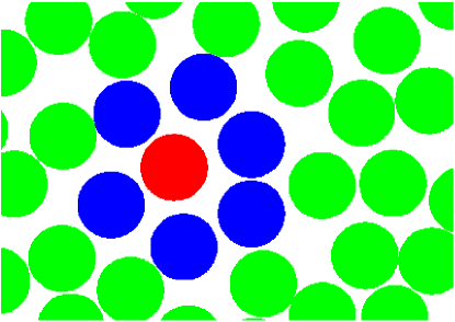
Figure 2: Positions of hard disks in two dimensions from a Monte Carlo simulation at a density close to freezing; courtesy of Th. Franosch. A particle and its shell of neighbours is highlighted by different colors/shadings.

Figure 2 shows a section of the cell of a Monte Carlo simulation of hard disks moving in two dimensions (for simplicity of visualization). The density is just below freezing and the sample was carefully equilibrated. Only 100 disks were simulated, so that finite size effects cannot be ruled out. Picking out a disk, it is surrounded by a shell of on average 6 neighbours (in two dimension, of 12 neighbours in three dimension), which hinder its free motion. In order for the central particle to diffuse at long times, it needs to escape the shell of neighbours. In order for a gap in this shell to open at higher concentrations, the neighbours have to be able to move somewhat themselves. Yet, each neighour is hindered by its own shell of neighbours, to which the originally picked particle belongs. Thus one can expect a cooperative feedback mechanism that with increasing density or particle interactions particle rearrangements take more and more time. It appears natural, that consequently stress fluctuations also slow down and the system becomes viscoelastic.

MCT appears to capture the cage-effect in supercooled liquids and predicts that it dominates the slow relaxation of structural correlations close to the glass transition Goe:91 ; Goe:92 . Density fluctuations play an important role because they are well suited to describe the structure of the particle system and its relaxation. Moreover, stresses that decay slowly because of the slow particle rearrangements, MCT argues, also can be approximated by density fluctuations using effective potentials. Density fluctuations not at large wavelengths, but for wavelengths corresponding to the average particle distance turn out to be the dominant ones. In agreement with the picture of the caging of particles by structural correlations, the MCT glass transition is independent on whether the particles move ballistically in between interactions with their neighbors (say collisions for hard spheres) or by diffusion. Structural arrest happens whenever the static density correlations for wavelengths around the average particle distance are strong enough. The arrest of structural correlations entails an increase in the viscosity of the dispersion connected to the existence of a slow Maxwell-process in the shear moduli. While the MCT solutions for density fluctuations have been thoroughly reviewed, the viscoelastic spectra have not been presented in such detail.

3.1 Shear moduli close to the glass transition

3.1.1 MCT equations and results for hard spheres

The loss and storage moduli of small amplitude oscillatory shear measurements Larson ; russel follow from Eq. (5b) in the linear response case at $\dot{\gamma}=0$:

$$G^{\prime}(\omega)+i\,G^{\prime\prime}(\omega)=i\omega\;\int_{0}^{\infty}dt\;e^{-i\,\omega\,t}\;g^{\text{lr}}(t)\;.$$ (16a)

Here, the shear modulus in the linear response regime is, again like the transient one in Eq. (5b), obtained from equilibrium averaging:

$$g^{\text{lr}}(t)=\frac{1}{k_{B}TV}\;\langle\,\sigma_{xy}\;e^{\Omega^{\dagger}_{e}t}\;\sigma_{xy}\,\rangle^{(\dot{\gamma}=0)}\;,$$ (16b)

yet, differently from the transient one, the equilibrium one contains the equilibrium SO $$\Omega_{e}$$, which characterizes the quiescent system:

$$\Omega_{e}=\sum_{j=1}^{N}D_{0}\;\frac{\partial}{\partial{\bf r}_{j}}\cdot\left(\frac{\partial}{\partial{\bf r}_{j}}-\frac{1}{k_{B}T}\,{\bf F}_{j}\right)\;,$$ (16c)

The linear response modulus thus quantifies the small stress fluctuations, which are excited by thermally, and relax because of Brownian motion.

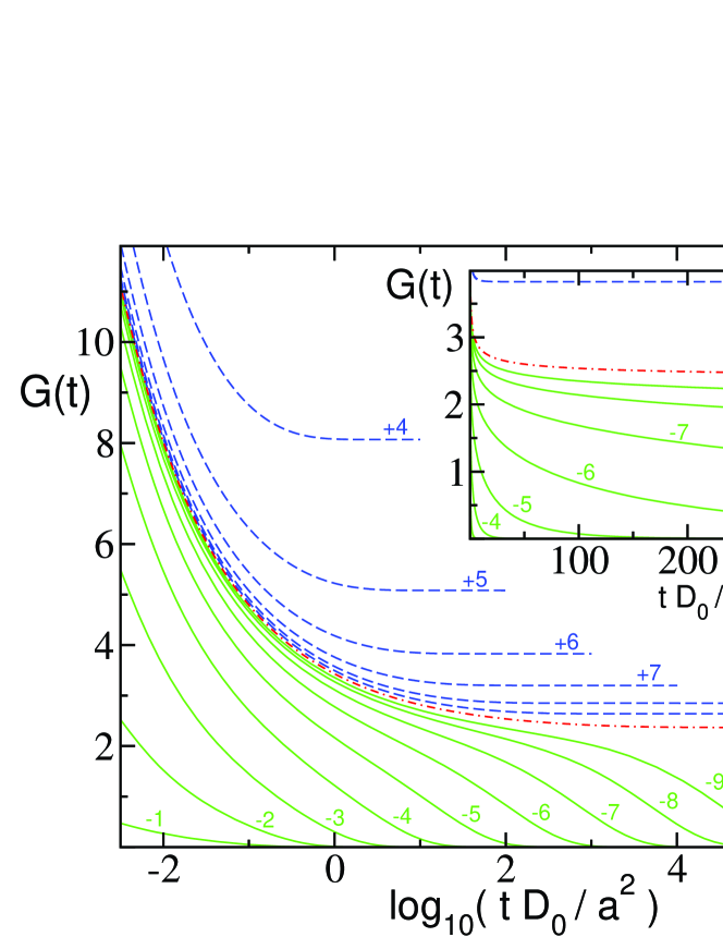
Figure 3: Equilibrium potential or linear response shear modulus $G(t)=g^{\text{lr}}(t)$ (in units of $k_{B}T/R_{H}^{3}$) for Brownian hard spheres with radius $a=R_{H}$ for packing fractions close to vitrification at $\phi_{c}$; from Ref. Fuc:05 . Densities are measured by the separation parameter $\varepsilon=(\phi-\phi_{c})/\phi_{c}=\pm 10^{-|n|/3}$, and labels denote the value $n$. Positive values belong to glass ($\varepsilon>0$), negative to fluid states ($\varepsilon<0$); the label $c$ gives the transition. The inset shows a subset of the curves on a linear time axis; the increase of $g^{\text{lr}}(t)$ for short times cannot be resolved.

Predictions of the (idealized) MCT equations for the potential part of the equilibrium, time-dependent shear modulus $g^{\text{lr}}(t)$ of hard spheres for various packing fractions $\phi$ are shown in Fig. 3 and calculated from the limit of Eq. (11d) for vanishing shear rate:

$$g^{\text{lr}}(t)\approx\frac{k_{B}T}{60\pi^{2}}\;\int_{0}^{\infty}\!\!dk\;k^{4}\;\left(\frac{\partial\ln{S_{k}}}{\partial k}\right)^{2}\;\Phi^{2}_{{k}}(t)\;,$$ (17)

The normalized density fluctuation functions are calculated self-consistently within MCT from the Eqs. (13,14) at vanishing shear rate Goe:91 ; Goe:92 , which turn into the quiescent MCT equations:

$$\partial_{t}\Phi_{q}(t)+\Gamma_{q}\;\left\{\Phi_{q}(t)+\int_{0}^{t}dt^{\prime}\;m_{q}(t-t^{\prime})\;\partial_{t^{\prime}}\,\Phi_{q}(t^{\prime})\right\}=0\;,$$ (18a)

where the initial decay rate $$\Gamma_{q}=D_{s}\,q^{2}/S_{q} D_{s} D_{0} D_{s}=D_{0} D_{s}\neq D_{0} {\bf p}={\bf q}-{\bf k}$$ describes diffusion with a short-time diffusion coefficient differing from the because of HI; will be taken for exemplary calculations, while is required for analyzing experimental data. The memory kernel becomes (again with abbreviation )

$$m_{q}(t)=\frac{1}{2N}\sum_{{\bf k}}V_{qkp}\;\Phi_{k}(t)\;\Phi_{p}(t)\;,$$ (18b)

$$V_{qkp}=\frac{S_{q}\,S_{k}\,S_{p}}{q^{4}}\;\left({\bf q}\cdot\left[\,{\bf k}\;nc_{k}+{\bf p}\;nc_{p}\,\right]\right)^{2}\;.$$ (18c)

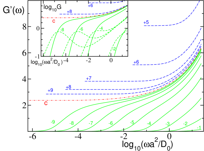
Figure 4: Storage part of the shear modulus $G^{\prime}(\omega)$ corresponding to Fig. 3. The inset shows storage and loss moduli (only for fluid states) for a number of densities.

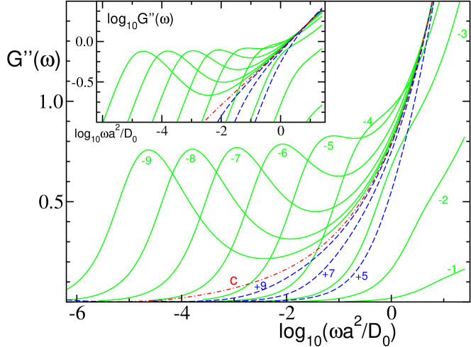
Figure 5: Loss part of the shear modulus $G^{\prime\prime}(\omega)$ corresponding to Fig. 3. The inset shows the same data in a double logarithmic representation.

Packing fractions are conveniently measured in relative separations $\varepsilon=(\phi-\phi_{c})/\phi_{c}$ to the glass transition point, which for this model of hard spheres lies at $\phi_{c}=0.516$ Goe:91 ; Fra:97 . Note that this result depends on the static structure factor $S(q)$ , which is taken from Percus-Yevick theory, and that the experimentally determined value $\phi_{c}^{\rm expt.}=0.58$ lies somewhat higher Meg:93 ; Meg:94 . The wavevector integrals were discretized using $M=100$ wavevectors chosen from $k_{\rm min}=0.1/R_{H}$ up to $k_{\rm max}=19.9/R_{H}$ with separation $\Delta k=0.2/R_{H}$ for Figs. 3 to 5, or using $M=600$ wavevectors chosen from $k_{\rm min}=0.05/R_{H}$ up to $k_{\rm max}=59.95/R_{H}$ with separation $\Delta k=0.1/R_{H}$ for Figs. 6 and 7, and in Sect. 6.2 in Fig. 23. Time was discretized with initial step-width $dt=2\,10^{-7}R_{H}^{2}/D_{s}$, which was doubled each time after 400 steps. Slightly different discretizations in time and wavevector of the MCT equations were used in Sects. 3.2.1 and 4, causing only small quantitative differences whose discussion goes beyond the present review. The quiescent density correlators $\Phi_{q}(t)$ corresponding to the following linear response moduli have thoroughly been discussed in Ref. Fra:97 .

For low packing fractions, or large negative separations, the modulus decays quickly on a time-scale set by the short-time diffusion of well separated particles. The strength of the modulus increases strongly at these low densities, and its behavior at short times presumably depends sensitively on the details of hydrodynamic and potential interactions; thus Fig. 3 is not continued to small times, where the employed model (taken from Ref. Fra:97 ; Fuc:99 ) is too crude . Approaching the glass transition from below, $\varepsilon\nearrow 0$, little changes in $g^{\text{lr}}(t)$ at short times, because the absolute change in density becomes small. Yet, at long times a process in $g^{\text{lr}}(t)$ becomes progressively slower upon taking $\varepsilon$ to zero. It can be considered the MCT analog of the phenomenological Maxwell-process. MCT finds that it depends on the equilibrium structural correlations only, while HI and other short time effects only shift its overall time scale. Importantly, this overall time scale applies to the slow process in coherent and incoherent density fluctuations as well as in the stress fluctuations Fra:98 . This holds even though e.g. HI are known to affect short time diffusion coefficients and high frequency viscosities differently. Upon crossing the glass transition, a part of the relaxation freezes out and the amplitude $G_{\infty}$ of the Maxwell-process does not decay; the modulus for long times approaches the elastic constant of the glass $g^{\text{lr}}(t\to\infty)\to G_{\infty}>0$. Entering deeper into the glassy phase the elastic constant increase quickly with packing fraction.

The corresponding storage $G^{\prime}(\omega)$ and loss $G^{\prime\prime}(\omega)$ moduli are shown as functions of frequency in Figs. 4 and 5, respectively. The slow Maxwell-process appears as a shoulder in $G^{\prime}$ which extends down to lower and lower frequencies when approaching glassy arrest, and reaches to zero frequency in the glass, $G^{\prime}(\omega=0)=G_{\infty}$. The slow process shows up as a peak in $G^{\prime\prime}$ which in parallel motion (see inset of Fig. 4) shifts to lower frequencies when $\varepsilon\nearrow 0$. Including hydrodynamic interactions into the calculation by adjusting $\eta_{\infty}$ would affect the frequency dependent moduli at higher frequencies only. For the range of smaller frequencies which is of interest here, only a small correction would arise.

3.1.2 Comparison with experiments

Recently, it has been demonstrated that suspensions of thermosensitive particles present excellent model systems for measuring the viscoelasticity of dense concentrations. The particles consist of a solid core of polystyrene onto which a thermosensitive network of poly(N-isopropylacrylamide) (PNIPAM) is attached Cra:06 ; Cra:08 . The PNiPAM shell of these particles swells when immersed in cold water (10 - 15^oC). Water gets expelled at higher temperatures leading to a considerable shrinking. Thus, for a given number density the effective volume fraction $\phi_{\text{eff}}$ can be adjusted within wide limits by adjusting the temperature. Senff et al. (1999) were the first to demonstrate the use of these particles as model system for studying the dynamics in concentrated suspensions Sen:99 ; Sen:99b . The advantage of these systems over the classical hard sphere systems are that dense suspensions can be generated in situ without shear and mechanical deformation. The previous history of the sample can be erased by raising the temperature and thus lowering the volume fraction to the fluid regime.

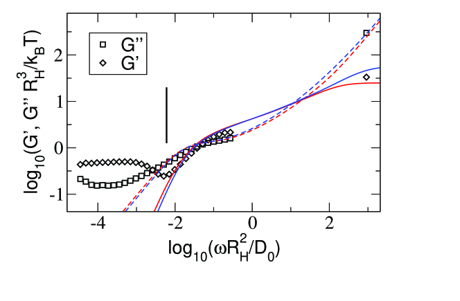
Figure 6: The reduced storage (diamonds and solid lines) and loss (squares and broken lines) modulus for a fluid state at effective packing fraction $\phi_{\rm eff}=0.540$; from Ref. Cra:08 . The vertical bars mark the minimal rescaled frequency above which the influence of crystallisation can be neglected. Parameters in the MCT calculation given as blue lines: $\varepsilon=-0.01$, $\frac{D_{S}}{D_{0}}=0.15$, and $\eta_{\infty}=0.3\,k_{B}T/(D_{0}R_{H})$; moduli scale factor $c_{y}=1.4$. For the other lines see Ref. Cra:08 .

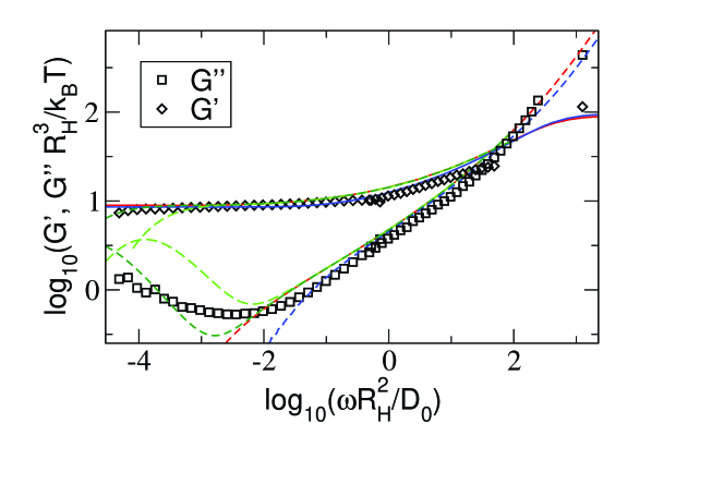
Figure 7: The moduli for a glass state at effective packing fraction $\phi_{\rm eff}=0.622$; storage (diamonds and solid lines) and loss (squares and broken lines) moduli from Cra:08 . MCT fits are shown as blue lines with parameters: $\varepsilon=0.03$, $\frac{D_{S}}{D_{0}}=0.08$, and $\eta_{\infty}=0.3\,k_{B}T/(D_{0}R_{H})$; moduli scale factor $c_{y}=1.4$ . For the other lines see Ref. Cra:08 .

Frequency dependent moduli were measured spanning a wide density and frequency range by combining different techniques. The moduli exhibit a qualitative change when increasing the effective packing fraction from around 50% to above 60%. For lower densities (see Fig. 6), the spectra $G^{\prime\prime}(\omega)$ exhibit a broad peak or shoulder, which corresponds to the final or $\alpha$-relaxation. Its peak position (or alternatively the crossing of the moduli, $G^{\prime}=G^{\prime\prime}$) is roughly given by $\omega\tau=1$ . These properties characterize a viscoelastic fluid. For higher density, see Fig. 7, the storage modulus exhibits an elastic plateau at low frequencies. The loss modulus drops far below the elastic one. These observations characterize a soft solid .

The linear response moduli are affected by the presence of small crystallites. At low frequencies, $G^{\prime}(\omega)$ and $G^{\prime\prime}(\omega)$ increase above the behavior expected for a solution ($G^{\prime}(\omega\to 0)\to\eta_{0}\,\omega$ and $G^{\prime\prime}(\omega\to 0)\to c\,\omega^{2}$) even at low density, and exhibit elastic contributions (apparent from $G^{\prime}(\omega)>G^{\prime\prime}(\omega)$); see Fig. 6. This effect tracks the crystallisation of the system during the measurement after a strong preshearing at $\dot{\gamma}=100$ $s^{-1}$. Only data can be considered which were collected before the crystallisation time; they lie to the right of the vertical bar in Fig. 6. While this experimental restriction limits more detailed studies of the shapes of the spectra close to the glass transition, the use of a system with a rather narrow size distribution provides the quantitatively closest comparison with MCT calculations for a monodisperse hard sphere system. Especially the magnitude of the stresses and the effective densities can be investigated quantitatively.

Included in figures 6 and 7 are calculations using the microscopic MCT given by Eqs. (16) to (18) evaluated for hard spheres in PY approximation. The only a priori unknown, adjustable parameter is a frequency or time scale, which was adjusted by varying the short time diffusion coefficient $D_{s}$ appearing in the initial decay rate in Eq. (18a). Values for $D_{s}/D_{0}$ are reported in the captions. The viscous contribution to the stress is mimicked by including $\eta_{\infty}$ like in Eq. (15); it can directly be measured at the highest frequencies. Gratifyingly, the stress values computed from the microscopic approach are close to the measured ones; they are too small by 40% only, which may arise from the approximate structure factors entering the MCT calculation; the Percus-Yevick approximation was used here russel . In order to compare the shapes of the moduli the MCT calculations were scaled up by a factor $c_{y}=1.4$ in Figs. 6 and 7. Microscopic MCT also does not hit the correct value for the glass transition point Goe:92 ; Goe:91 . It finds $\phi^{\rm MCT}_{c}=0.516$, while experiments give $\phi^{\rm exp}_{c}\approx 0.58$. Thus, when comparing, the relative separation from the respective transition point needs to be adjusted as, obviously, the spectra depend sensitively on the distance to the glass transition; the fitted values of the separation parameter $\varepsilon$ are included in the captions.

Overall, the semi-quantitative agreement between the linear viscoelastic spectra and first-principles MCT calculations is very promising. Yet, crystallization effects in the data prevent a closer look, which will be given in Section 6.2, where data from a more polydisperse sample are discussed.

3.2 Distorted structure factor

3.2.1 Linear order in $\dot{\gamma}$

The stationary structural correlations of a dense fluid of spherical particles undergoing Brownian motion, neglecting hydrodynamic interactions, change with shear rate $\dot{\gamma}$ in response to a steady shear flow. In linear order, the structure is distorted only in the plane of the flow, while already in second order in $\dot{\gamma}$, the structure factor changes under shear also for wavevectors lying in the plane perpendicular to the flow. Consistent with previous theories, MCT-ITT finds regular expansion coefficients in linear and quadratic order in $\dot{\gamma}$ for fluid (ergodic) suspensions Hen:07 . For the steady state structure factor $S_{\bf q}{(\dot{\gamma})}$ of density fluctuations under shearing in plain Couette flow defined in Eq. (6a), the change from the equilibrium one in linear order in shear rate is given by the following ITT-approximation:

$$S_{q}{(\dot{\gamma})}=S_{q}+\dot{\gamma}\,\left\{\frac{q_{x}q_{y}}{q}S^{\prime}_{q}\,\int_{0}^{\infty}\!\!\!\!\!dt\;\Phi_{q}^{2}(t)\right\}+{\cal O}(\text{Pe}^{2})\;.$$ (19)

This relation follows from Eq. (11a) in the limit of small $\dot{\gamma}$, where the quiescent density correlators can be taken from quiescent MCT in Eq. (18).

3.2.2 Comparison with simulations

Figure 8 shows the contribution $\delta S_{\bf q}^{(\dot{\gamma}}$ to the distorted structure factor in leading linear order in $\dot{\gamma}$ for packing fractions $\phi=0.36,0.44$ and $0.46$. Data taken from Brownian dynamics simulations at $\phi=0.43$ and $0.5$ from Ref. Szamel01 are also included. In both cases the data was divided by a factor $\dot{\gamma}q_{x}q_{y}/q^{2}$ which is the origin of the trivial anisotropy in the leading linear order. The distortion $\delta S_{\bf q}^{(\dot{\gamma})}$ of the microstructure grows strongly with $\phi$, because of the approach to the glass transition. The $\delta S_{\bf q}^{(\dot{\gamma})}$ is proportional to the $\alpha$-relaxation time $\tau$, as proven in the left inset of Fig. 8. Here, $\tau$ is estimated from $\Phi_{q_{p}}(t=\tau)=0.1$, where $q_{p}$ denotes the position of the primary peak in $S_{q}$. Rescaling the data with Pe, collapses the curves at different distances to the glass transition. The strongest shear-dependence occurs for the direction of the extensional component of the flow, $q_{x}=q_{y}$. Here, the mesoscale order of the dispersion grows; the peak in $\delta S_{\bf q}^{(\dot{\gamma})}$ increases and sharpens. The ITT results qualitatively agree with the simulations in these aspects Szamel01 .

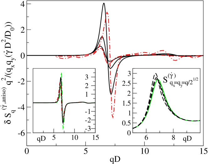
Figure 8: Contribution $\delta S_{\bf q}^{\dot{\gamma}}$ linear in shear rate to the distorted structure factor $S_{\bf q}(\dot{\gamma})$ normalized to $\dot{\gamma}q_{x}q_{y}/q^{2}$ (black solid lines); from Ref. Hen:07 , here $D$ denotes the hard sphere diameter. Decreasing the relative separations from the critical point as $\varepsilon=-0.2,-0.15,-0.1$, the magnitude of $\delta S_{\bf q}^{(\dot{\gamma})}$ increases. The dashed-dotted red curves are Brownian dynamics simulation data from Ref. Szamel01 using the same normalization at $\varepsilon=-0.259,-0.138$. The right inset shows the unnormalized $S_{\bf q}^{(\dot{\gamma})}$ along the extensional axis $q_{x}=q_{y}=q/\sqrt{2}$ at $\varepsilon=-0.1$ and, from bottom to top, Pe $=\dot{\gamma}\tau=0$ (green-solid), $1/8$, $1/4$ and $1/2$ (all black-dashed), where $\Phi_{q_{p}}(t=\tau)=0.1$ defines $\tau$. Pe$/$Pe${}_{0}=1.66$ holds at this $\varepsilon$. The left inset shows the data of the main figure rescaled with the dressed Peclet number, $\delta S_{\bf q}^{(\dot{\gamma},{\rm aniso})}/({\rm Pe}\,q_{x}q_{y}/q^{2}$); for $\varepsilon=-0.1,-0.05$, and $-0.01$ (with increasing peak height) the values Pe/Pe${}_{0}=1.66$, Pe/Pe${}_{0}=8.06$, and Pe/Pe${}_{0}=419$ are used.

The most important finding of Fig. 8 concerns the magnitude of the distortion of the microstructure, and the dimensionless parameter measuring the effect of shear relative to the intrinsic particle motion. This topic can already be discussed using the linear order result, and is not affected by considerations of hydrodynamic interactions, as can be glanced from comparing Brownian dynamics simulations Szamel01 and experiments on dissolved particles Johnson88 . In previous theories, shear rate effects enter when the bare Peclet number Pe₀ becomes non-negligible. In the present ITT approach the dressed Peclet/ Weissenberg number Pe$=\dot{\gamma}\tau$ governs shear effects; here, $\tau$ is the (final) structural relaxation time. Shear flow competes with structural rearrangements that become arbitrarily slow compared to diffusion of dilute particles when approaching the glass transition. The distorted microstructure results from the competition between shear flow and cooperative structural rearrangements. It is thus no surprise that previous theories using Pe₀, which is characteristic for dilute fluids or strong flows, had severely underestimated the magnitude of shear distortions in hard sphere suspensions for higher packing fractions; Refs. Szamel01 ; lionberger report an underestimate by roughly a decade at $\phi=0.50$. The ITT approach actually predicts a divergence of $\lim_{\dot{\gamma}\to 0}(S_{\bf q}^{(\dot{\gamma})}-S_{q})/\dot{\gamma}$ for density approaching the glass transition at $\phi_{c}\approx 0.58$. And for (idealized) glass states, where $\tau=\infty$ holds in MCT following Maxwell’s phenomenology, the stationary structure factor becomes non-analytic, and differs from the equilibrium one even for $\dot{\gamma}\to 0$. The distortion $\delta S^{(\dot{\gamma})}_{{\bf q}}$ thus qualitatively behaves like the stress, which goes to zero linear in $\dot{\gamma}$ in the fluid, but approaches a yield stress $\sigma^{+}$ in the glass for $\dot{\gamma}\to 0$.

The reassuring agreement of ITT results on $S_{\bf q}^{(\dot{\gamma})}$ with the data from simulations and experiments shows that in the ITT approach the correct expansion parameter Pe has been identified. This can be taken as support for the ITT-strategy to connect the non-linear rheology of dense dispersions with the structural relaxation studied at the glass transition.

4 Universal aspects of the glass transition in steady shear

The summarized microscopic MCT-ITT equations contain a non-equilibrium transition between a shear thinning fluid and a shear-molten glassy state; it is the central novel transition found in MCT-ITT Fuc:02 . Close to the transition, (rather) universal predictions can be made about the non-linear dispersion rheology and the steady state properties. Following Refs. Fuc:03 ; Cra:08 , the central predictions are introduced in this section and summarized in the overview figure 9; the following results sections contain more examples. Figure 9 is obtained from the schematic model which is also often used to analyse data, and which is introduced in the following section 5.2 .

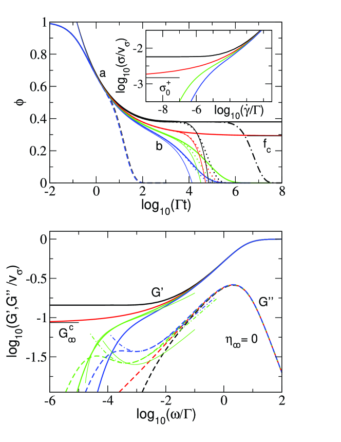
Figure 9: Overview of the properties of the F${}_{12}^{(\dot{\gamma})}$-model characteristic for the transition between fluid and yielding glass; from Ref. Cra:08 . The upper panel shows numerically obtained transient correlators $\Phi(t)$ for $\varepsilon=0.01$ (black curves), $\varepsilon=0$ (red), $\varepsilon=-0.005$ (green), and $\varepsilon=-0.01$ (blue). The shear rates are $\left|\dot{\gamma}/\Gamma\right|=0$ (thick solid lines), $\left|\dot{\gamma}/\Gamma\right|=10^{-6}$ (dotted lines), and $\left|\dot{\gamma}/\Gamma\right|=10^{-2}$ (dashed lines). For the glass state at $\varepsilon=0.01$ (black), $\left|\dot{\gamma}/\Gamma\right|=10^{-8}$ (dashed-dotted-line) is also included. All curves were calculated with $\gamma_{c}=0.1$ and $\eta_{\infty}=0$. The thin solid lines give the factorization result Eq. (20) with scaling functions $\cal G$ for $\left|\dot{\gamma}/\Gamma\right|=10^{-6}$; label $a$ marks the critical law (22b), and label $b$ marks the von Schweidler-law (23). The critical glass form factor $f_{c}$ is indicated. The inset shows the flow curves for the same values for $\varepsilon$. The thin black bar shows the yield stress $\sigma^{+}_{c}$ for $\varepsilon=0$. The lower panel shows the viscoelastic storage (solid line) and loss (broken line) modulus for the same values of $\varepsilon$. The thin green lines are the Fourier-transformed factorization result Eq. (20) with scaling function $\cal G$ taken from the upper panel for $\varepsilon=-0.005$. The dashed-dotted lines show the fit formula Eq. (24) for the spectrum in the minimum-region with $G_{\rm min}/v_{\sigma}=0.0262$, $\omega_{\rm min}/\Gamma=0.000457$ at $\varepsilon=-0.005$ (green) and $G_{\rm min}/v_{\sigma}=0.0370$, $\omega_{\rm min}/\Gamma=0.00105$ at $\varepsilon=-0.01$ (blue). The elastic constant at the transition $G_{\infty}^{c}$ is marked also, while the high frequency asymptote $G^{\prime}_{\infty}=G^{\prime}(\omega\to\infty)$ is not labeled explicitly.

A dimensionless separation parameter $\varepsilon$ measures the distance to the transition which lies at $\varepsilon=0$. A fluid state ($\varepsilon<0$) possesses a (Newtonian) viscosity, $\eta_{0}(\varepsilon<0)=\lim_{\dot{\gamma}\to 0}\sigma(\dot{\gamma})/\dot{\gamma}$, and shows shear-thinning upon increasing $\dot{\gamma}$. Via the relation $\eta_{0}=\lim_{\omega\to 0}\,G^{\prime\prime}(\omega)/\omega$, the Newtonian viscosity can also be taken from the linear response loss modulus at low frequencies, where $G^{\prime\prime}(\omega)$ dominates over the storage modulus. The latter varies like $G^{\prime}(\omega\to 0)\sim\omega^{2}$. A glass ($\varepsilon\geq 0$), in the absence of flow, possesses an elastic constant $G_{\infty}$, which can be measured in the elastic shear modulus $G^{\prime}(\omega)$ in the limit of low frequencies, $G^{\prime}(\omega\to 0,\varepsilon\geq 0)\to G_{\infty}(\varepsilon)$. Here the storage modulus dominates over the loss one, which drops like $G^{\prime\prime}(\omega\to 0)\sim\omega$. The high frequency modulus $G^{\prime}_{\infty}=G^{\prime}(\omega\to\infty)$ is characteristic of the particle interactions, see Footnote 4, and exists, except for the case of hard sphere interactions without HI, in fluid and solid states. The dissipation at high frequencies $G^{\prime\prime}(\omega\to\infty)\to\eta_{\infty}\omega$ also shows no anomaly at the glass transition and depends strongly on HI and solvent friction.

Enforcing steady shear flow melts the glass. The stationary stress of the shear-molten glass always exceeds a (dynamic) yield stress. For decreasing shear rate, the viscosity increases like $1/\dot{\gamma}$, and the stress levels off onto the yield-stress plateau, $\sigma(\dot{\gamma}\to 0,\varepsilon\geq 0)\to\sigma^{+}(\varepsilon)$.

Close to the transition, the zero-shear viscosity $\eta_{0}$, the elastic constant $G_{\infty}$, and the yield stress $\sigma^{+}$ show universal anomalies as functions of the distance to the transition.

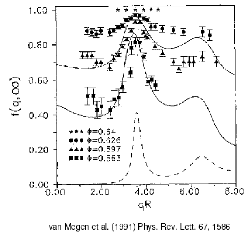
Figure 10: Glass form factors $f_{q}$ as function of wavevector $q$ in a colloidal glass of hard spheres for packing fractions $\phi$ as labeled. Data obtained by van Megen and coworkers by dynamic light scattering are qualitatively compared to MCT computations using the PY-$S_{q}$ at $\phi$ values chosen ad hoc to match the experimental data; from Meg:91 . The PY structure factor at the glass transition density $\phi=0.58$ is shown as broken line, rescaled by a factor $1/10$ .

The described results follow from the stability analysis of Eqs. (13,14) around an arrested, glassy structure $f_{q}$ of the transient correlator Fuc:02 ; Fuc:03 . Considering the time window where $\Phi_{\bf q}(t)$ is close to arrest at $f_{q}$, and taking all control parameters like density, temperature, etc. to be close to the values at the transition, the stability analysis yields the ’factorization’ between spatial and temporal dependences

$$\Phi_{\bf q}(t)=f^{c}_{q}+h_{q}\;{\cal G}(\,t/t_{0},\varepsilon,\dot{\gamma}t_{0}\,)+\ldots\;,$$ (20)

where the (isotropic) glass form factor $f^{c}_{q}$ and critical amplitude $h_{q}$ describe the spatial properties of the metastable glassy state. The critical glass form factor $f^{c}_{q}$ gives the long-lived component of density fluctuations right at the transition $\varepsilon=0$, while $\Phi_{\bf q}(t\to\infty,\varepsilon\geq 0,\dot{\gamma}=0)=f_{q}>0$ characterizes states even deep in the glass with $f_{q}$ obeying Goe:91 :

$$\frac{f_{q}}{1-f_{q}}=\frac{1}{2N}\sum_{\bf k}\;V_{qkp}\;f_{k}\;f_{p}\;,$$ (21)

with $V_{qkp}$ from Eq. (18c) as follows from Eqs. (13,14) asymptotically in the limit of vanishing shear rate Fuc:03 . Figure 10 shows dynamic light scattering data for the glass form factors at a number of densities in PMMA hard sphere colloids, comparing them to solutions of Eq. (21) evaluated for hard spheres using the PY structure factor; it is included in Fig. 10 for the packing fraction $\phi_{c}=0.58$ of the experimental glass transition. The glass form factor varies with the average particle separation and in phase with the structure factor. Both, $f_{q}$ and $h_{q}$ thus describe local correlations, the so-called ’cage-effect’, and can be taken as constants independent on shear rate and density, as they are evaluated from the vertices in Eq. (14) at the transition point $(\varepsilon=0,\dot{\gamma}=0)$.

All time-dependence and (sensitive) dependence on the external control parameters is contained in the function $\cal G$, which often is called ’$\beta$-correlator’ and obeys the non-linear stability equation Fuc:02 ; Fuc:03 ; Fuc:09

$$\tilde{\varepsilon}-c^{(\dot{\gamma})}\;(\dot{\gamma}t)^{2}+\lambda\;{\cal G}^{2}(t)=\frac{d}{dt}\int_{0}^{t}\!\!\!dt^{\prime}\;{\cal G}(t-t^{\prime})\;{\cal G}(t^{\prime})\;,$$ (22a)

with initial condition

$${\cal G}(t\to 0)\to(t/t_{0})^{-a}\;.$$ (22b)

The two parameters $\lambda$ and $c^{(\dot{\gamma})}$ in Eq. (22a) are determined by the static structure factor at the transition point, and take values around $\lambda\approx 0.73$ and $c^{(\dot{\gamma})}\approx 0.7$ for the PY $S_{q}$ for hard spheres. The transition point then lies at packing fraction $\phi_{c}=\frac{4\pi}{3}n_{c}R_{H}^{3}\approx 0.52$ (index $c$ for critical), and the separation parameter measures the relative distance, $\tilde{\varepsilon}=C\,\varepsilon$ with $\varepsilon=(\phi-\phi_{c})/\phi_{c}$ and $C\approx 1.3$. The ’critical’ exponent $a$ is given by the exponent parameter $\lambda$ via $\lambda=\Gamma(1-a)^{2}/\Gamma(1-2a)$, as had been found in quiescent MCT Goe:91 ; Goe:92 .

The time scale $t_{0}$ in Eq. (22b) provides the means to match the function ${\cal G}(t)$ to the microscopic, short-time dynamics. The Eqs. (13,14) contain a simplified description of the short time dynamics in colloidal dispersions via the initial decay rate $\Gamma_{\bf q}(t)$. From this model for the short-time dynamics, the time scale $t_{0}\approx 1.6\,10^{-2}R_{H}^{2}/D_{0}$ is obtained. Solvent mediated effects on the short time dynamics are well known and are neglected in $\Gamma_{\bf q}(t)$ in Eq. (13). The most simple minded approximation to account for HI is given in Eq. (15). It only shifts the value of $t_{0}$. Within the ITT approach, this finding holds more generally. Even if HI lead to more substantial changes of Eq. (13), all of the mentioned universal predictions would remain true, as long as HI do not affect the mode coupling vertex in Eq. (14). Like in the quiescent MCT Fra:98 , in MCT-ITT hydrodynamic interactions can thus be incorporated into the theory of the glass transition under shear, and amount to a rescaling of the matching time $t_{0}$, only.

The parameters $\varepsilon$, $\lambda$ and $c^{(\dot{\gamma})}$ in Eq. (22a) can be determined from the equilibrium structure factor $S_{q}$ at or close to the transition, and, together with $t_{0}$ and the shear rate $\dot{\gamma}$ they capture the essence of the rheological anomalies in dense dispersions. A divergent viscosity follows from the prediction of a strongly increasing final relaxation time in $\cal G$ in the quiescent fluid phase Goe:92 ; Goe:91 :

$${\cal G}(t\to\infty,\varepsilon<0,\dot{\gamma}=0)\to-\left(t/\tau\right)^{b}\quad,\;\;\mbox{with }\;\frac{t_{0}}{\tau}\propto(-\varepsilon)^{\gamma}\;.$$ (23)

The entailed temporal power law, termed von Schweidler law, initiates the final decay of the correlators, which has a density and temperature independent shape $\tilde{\Phi}_{q}(\tilde{t})$. In MCT, the (full) correlator thus takes the characteristic form of a two-step relaxation. The final decay, often termed $\alpha$-relaxation, depends on $\varepsilon$ only via the time scale $\tau(\varepsilon)$ which rescales the time, $\tilde{t}=t/\tau$. Equation (22) establishes the crucial time scale separation between $t_{0}$ and $\tau$, the divergence of $\tau$, and the stretching (non-exponentiality) of the final decay; it also gives the values of the exponents via $\lambda=\Gamma(1+b)^{2}/\Gamma(1+2b)$, and $\gamma=(1/a+1/b)/2$. Using Eq. (17), the MCT-prediction for the divergence of the Newtonian viscosity follows Goe:92 ; Goe:91 . During the final decay the quiescent shear modulus also becomes a function of rescaled time, $\tilde{t}=t/\tau$, leading to $\eta_{0}\propto\tau(\varepsilon)$; its initial value is given by the elastic constant at the transition, $G_{\infty}^{c}$.

The two asymptotic temporal power-laws of MCT also affect the frequency dependence of $G^{\prime\prime}$ in the minimum region. The scaling function $\cal G$ describes the minimum as crossover between two power laws in frequency. The approximation for the modulus around the minimum in the quiescent fluid becomes Goe:91 :

$$G^{\prime\prime}(\omega)\approx\frac{G_{\rm min}}{a+b}\;\left[\,b\,\left(\frac{\omega}{\omega_{\rm min}}\right)^{a}+a\,\left(\frac{\omega_{\rm min}}{\omega}\right)^{b}\,\right]\;.$$ (24)

The parameters in this approximation follow from Eqs. (22,23) which give $G_{\rm min}\propto\sqrt{-\varepsilon}$ and $\omega_{\rm min}\propto(-\varepsilon)^{1/2a}$. Observation of this handy expression requires that the relaxation time $\tau$ is (very) large, viz. that time scale separation holds (extremely well) for (very) small $-\varepsilon$; even in the exemplary Fig. 9, the chosen distances to the glass transition are too large in order for the Eq. (24) to agree with the true $\beta$-correlator $\cal G$, which is also included in Fig. 9. The reason for this difficulty is the aspect that the expansion in Eq. (20) is an expansion in $\sqrt{\varepsilon}$, which requires very small separation parameters $\varepsilon$ for corrections to be negligible. For packing fractions too far below the glass transition, the final relaxation process is not clearly separated from the high frequency relaxation. This holds in the experimental data shown in Fig. 6, where the final structural decay process only forms a shoulder.

On the glassy side of the transition, $\varepsilon\geq 0$, the transient density fluctuations stays close to a plateau value for intermediate times which increases when going deeper into the glass,

$${\cal G}(t_{0}\ll t\ll 1/|\dot{\gamma}|,\varepsilon\geq 0)\to\sqrt{\frac{\tilde{\varepsilon}}{1-\lambda}}+{\cal O}(\varepsilon)\;.$$ (25)

Entered into Eq. (17), the square-root dependence of the plateau value translates into the square-root anomaly of the elastic constant $G_{\infty}$, and causes the increase of the yield stress close to the glass transition.

Only, for vanishing shear rate, $\dot{\gamma}=0$, an ideal glass state exists in the ITT approach for steady shearing. All density correlators arrest at a long time limit, which from Eq. (25) close to the transition is given by $\Phi_{\bf q}(t\to\infty,\varepsilon\geq 0,\dot{\gamma}=0)=f_{q}=f^{c}_{q}+h_{q}\sqrt{\tilde{\varepsilon}/(1-\lambda)}+{\cal O}(\varepsilon)$. Consequently the modulus remains elastic at long times, $g(t\to\infty,\varepsilon\geq 0,\dot{\gamma}=0)=G_{\infty}>0$. Any (infinitesimal) shear rate, however, melts the glass and causes a final decay of the transient correlators. The function $\cal G$ initiates the decay around the critical plateau of the transient correlators and sets the common time scale for the final decay under shear

$${\cal G}(t\to\infty)\to-\sqrt{\frac{c^{(\dot{\gamma})}}{\lambda-\frac{1}{2}}}\;|\dot{\gamma}t|\equiv-\frac{t}{\tau_{\dot{\gamma}}}\;,\quad\text{ with }\;\tau_{\dot{\gamma}}=\sqrt{\frac{\lambda-\frac{1}{2}}{c^{(\dot{\gamma})}}}\;\frac{1}{|\dot{\gamma}|}\;.$$ (26)

Under shear all correlators decay from the plateau as function of $|\dot{\gamma}t|$; see e.g. Figs. 11, 12, 21 and 22. Steady shearing thus prevents non-ergodic arrest and restores ergodicity. Shear melts a glass and produces a unique steady state at long times. This conclusion is restricted by the already discussed assumption to neglect aging of glassy states. It could remain because of non-ergodicity in the initial quiescent state, which needs to be shear-molten before ITT holds. Ergodicity of the sheared state, however, suggests aging to be unimportant under shear, and that it should be possible to melt initial non-ergodic contributions Ber:00 ; Fie:00 . The experiments in model colloidal dispersions reported in Sect. 3.1.2 and Sect. 6.2 support this notion, as history independent steady states could be achieved at all densities.

The described universal scenario of shear-molten glass and shear-thinnig fluid makes up the core of the MCT-ITT predictions derived from Eqs. (11) to (14). Their consequences for the nonlinear rheology will be discussed in more detail in the following sections, while the MCT results for the linear viscoelasticity were reviewed in Sect. 3. Yet, the anisotropy of the equations has up to now prevented more complete solutions of the MCT-ITT equations of Sect. 2. Therefore, simplified MCT-ITT equations become important, which can be analysed in more detail and recover the central stability equations Eqs. (20,22). The two most important ones will be reviewed next, before the theoretical picture is tested in comparison with experimental and simulations’ data.

5 Simplified models

Two progressively more simplified models provide insights into the generic scenario of non-Newtonian flow, shear melting and solid yielding which emerge from the ITT approach.

5.1 Isotropically sheared hard sphere model

On the fully microscopic level of description of a sheared colloidal suspension, affine motion of the particles with the solvent leads to anisotropic dynamics. Yet, recent simulation data of steady state structure factors indicate a rather isotropic distortion of the structure for Pe${}_{0}\ll 1$, even though the Weissenberg number Pe is already large Ber:02 ; Var:06 . Confocal microscopy data on concentrated solutions support this observation Bes:07 . The shift of the advected wavevector in Eq. (7) with time to higher values, intially is anisotropic, but becomes isotropic at longer times, when the magnitude of $q(t)$ increases along all directions. As the effective potentials felt by density fluctuations evolve with increasing wavevector, this leads to a decrease of friction functions, speed-up of structural rearrangements and shear-fluidization. Therefore, one may hope that an ’isotropically sheared hard spheres model’ (ISHSM), which for $\dot{\gamma}=0$ exhibits the nonlinear coupling of density correlators with wavelength equal to the average particle distance (viz. the “cage-effect”), and which, for $\dot{\gamma}\neq 0$, incorporates shear-advection, captures some spatial aspects of shear driven decorrelation.

5.1.1 Definition of the ISHSM

Thus, in the ISHSM, the equation of motion for the density fluctuations at time $t$ after starting the shear is approximated by the one of the quiescent system, namely Eq. (18a) (with $\Gamma_{q}=q^{2}D_{s}/S_{q}$). The memory function also is taken as isotropic and modeled close to the unsheared situation Fuc:02 ; Fuc:03

$$m_{q}(t)\approx\frac{1}{2N}\sum_{{\bf k}}V^{(\dot{\gamma})}_{qkp}(t)\;\Phi_{k}(t)\,\Phi_{p}(t)\;,$$ (27a)

with

$$V^{(\dot{\gamma})}_{qkp}(t)=\frac{n^{2}S_{q}S_{k}S_{p}}{q^{4}}\left[{\bf q}\cdot{\bf k}\;c_{\bar{k}(t)}+{\bf q}\cdot{\bf p}\;c_{\bar{p}(t)}\right]\left[{\bf q}\cdot{\bf k}\;c_{k}+{\bf q}\cdot{\bf p}\;c_{p}\right]$$ (27b)

where $${\bf p}={\bf q}\!-\!{\bf k} \bar{k}(t)=k(1+(t\dot{\gamma}/\gamma_{c})^{2})^{1/2} \bar{p}(t) \gamma_{c}$$, and the length of the advected wavevectors is approximated by and equivalently for . Note, that the memory function thus only depends on one time, and that shear advection leads to a dephasing of the two terms in the vertex Eq. (27b), which form a perfect square in the quiescent vertex of Eq. (18c) without shear. This (presumably) also is the dominant effect of shear in the full microscopic MCT-ITT memory kernel in Eq. (14). The fudge factor is introduced in order to correct for the underestimate of the effect of shearing in the ISHSM .

The expression for the potential part of the transverse stress may be simplified to

$$\sigma=\dot{\gamma}\;\int_{0}^{\infty}\!\!dt\;g(t,\dot{\gamma})\;,\;\text{with }\;g(t,\dot{\gamma})\approx\frac{k_{B}T}{60\pi^{2}}\;\int\!\!dk\;\frac{k^{5}\,c^{\prime}_{k}\;S^{\prime}_{\breve{k}(t)}}{\breve{k}(t)S_{k}^{2}}\;\Phi_{\breve{k}(t)}^{2}(t)\;,$$ (27c)

where, in the last equation Eq. (27c), the advected wavevector is chosen as $\breve{k}(t)=k(1+(t\dot{\gamma})^{2}/3)^{1/2}$ , as follows from straight forward isotropic averaging of ${\bf k}(t)$ . For the numerical solution of the ISHSM for hard spheres using $S_{q}$ in PY approximation, the wavevector integrals were discretized as discussed in Sect. 3.1.1 and following Ref. Fra:97 , using $M=100$ wavevectors from $k_{\rm min}=0.1/R$ up to $k_{\rm max}=19.9/R$ with separation $\Delta k=0.2/R$. Again, time was discretized with initial step-width $dt=2\,10^{-7}R^{2}/D_{s}$, which was doubled each time after 400 steps Fuc:91 . The model’s glass transition lies at $\phi_{c}=0.51591$, with exponent parameter $\lambda=0.735$ and $c^{(\dot{\gamma})}\approx 0.45/\gamma_{c}^{2}$ ; note that these values still change somewhat if the discretization is made finer. The separation parameter $\varepsilon=(\phi-\phi_{c})/\phi_{c}$), and $\dot{\gamma}$ are the two relevant control parameters determining the rheology.

5.1.2 Transient correlators

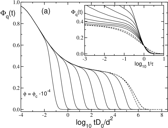
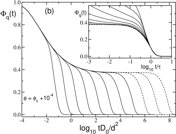
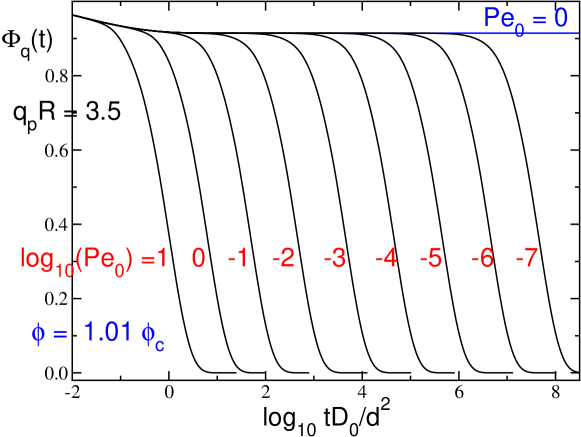
Figure 11: Normalized transient density correlators $\Phi_{q}(t)$ of the ISHSM at wavevector $q=3.4/d$ below (panel (a) at $\phi=\phi_{c}-10^{-4}$) and above (panel (b) at $\phi=\phi_{c}+10^{-4}$) the transition for increasing shear rates Pe${}_{0}=9^{n}*10^{-8}$ with $n=0,\ldots,10$ from right to left; the distances correspond to $\varepsilon=\pm 10^{-3.53}$. Curves for $n=$ 9, 10 carry short and for $n=$ 8 long dashes; note the collapse of the two short dashed curves in (a). The insets show the data rescaled so as to coincide at $\Phi(t=\tau)=0.1$. Panel (c) shows glass correlators at another wavevector $q=7/d$ for parameters as labeled; from Ref. Fuc:03 .

The shapes of the transient density fluctuation functions can be studied with spatial resolution in the ISHSM. Figure 11 displays density correlators at two densities, just below (panel (a)) and just above (panels (b,c)) the transition, for varying shear rates. Panel (b) and (c) compare correlators at different wavevectors to exemplify the spatial variation. In almost all cases the shear rate is so small that the bare Peclet number Pe₀ is negligibly small and the short-time dynamics is not affected.

Figure 12: Transient non-Newtonian shear modulus $g(t,\dot{\gamma})$ of the ISHSM in units of $k_{B}T/d^{3}$ for the packing fractions $\phi=\phi_{c}\pm 10^{-3}$ ($\varepsilon=\pm 10^{-2.53}$; dashed/ dotted lines, respectively) for increasing shear rates Pe${}_{0}=9^{n}*10^{-6}$ with $n=0,\ldots,8$ from right to left; note the collapse of fluid lines for the smallest Pe₀; from Ref. Fuc:03 . The solid line gives $g(t,\dot{\gamma})$ for $\phi=\phi_{c}$ and Pe${}_{0}=10^{-6}$. The inset shows the data rescaled so as to coincide at $g(t=\tau,\dot{\gamma})=5$; note the collapse of the $n=$ 6,7 & 8 curves for both $\phi>\phi_{c}$ and $\phi<\phi_{c}$.

In the fluid case, the final or $\alpha$-relaxation is also not affected for the two smallest dressed Peclet Pe values, but for larger Pe it becomes faster and less stretched; see the inset of fig. 11(a).

Above the transition, the quiescent system forms an (idealized) glass Goe:91 ; Goe:92 , whose density correlators arrest at the glass form factors $f_{q}$ from Fig. 10, and which exhibits a finite elastic constant $G_{\infty}$, that describes the (zero-frequency) Hookian response of the amorphous solid to a small applied shear strain $\gamma$: $\sigma=G_{\infty}\gamma$ for $\gamma\to 0$; the plateau $G_{\infty}$ can be seen in Fig. 3 and, for intermediate times in Fig. 12. If steady flow is imposed on the system, however, the glass melts for any arbitrarily small shear rate. Particles are freed from their cages and diffusion perpendicular to the shear plane also becomes possible. Any finite shear rate, however small, sets a finite longest relaxation time, beyond which ergodicity is restored; see Figs. 11(b,c) and 12.

The glassy curves at $\varepsilon>0$, panels (b,c), exhibit a shift of the final relaxation with $\tau_{\dot{\gamma}}$ from Eq. (26) and asymptotically approach a scaling function $\Phi_{q}^{+}(t/\tau_{\dot{\gamma}})$. The master equation for the “yielding” scaling functions $\Phi_{q}^{+}$ in the ISHSM can be obtained from eliminating the short-time dynamics in Eq. (18a). After a partial integration, the equation with $\partial_{t}\Phi_{q}(t)=0$ is solved by the scaling functions:

$$\Phi_{q}^{+}(\tilde{t})=m^{+}_{q}(\tilde{t})-\frac{d}{d\tilde{t}}\,\int_{0}^{\tilde{t}}d\tilde{t}^{\prime}\;m^{+}_{q}(\tilde{t}-\tilde{t}^{\prime})\;\Phi_{q}^{+}(\tilde{t}^{\prime})\;,$$ (28a)

where $$\tilde{t}=t/\tau_{\dot{\gamma}}$$, and the memory kernel is given by

$$m^{+}_{q}(\tilde{t})=\frac{1}{2N}\sum_{{\bf k}}V^{(\tilde{\dot{\gamma}})}_{q,{\bf k}}(\tilde{t})\;\Phi^{+}_{k}(\tilde{t})\,\Phi^{+}_{|{\bf q}-{\bf k}|}(\tilde{t})\;.$$ (28b)

While the vertex is evaluated at fixed shear rate, $$\tilde{\dot{\gamma}}=\sqrt{\frac{\lambda-\frac{1}{2}}{c^{(\dot{\gamma})}}}$$, it depends on the equilibrium parameters. The initialization for the correlator is given by

$$\Phi_{q}^{+}(\tilde{t}\to 0)=f_{q}\;,$$ (28c)

with glass form factor taken from Eq. (21). The two-step relaxation and the shift of the final relaxation with $$\tau_{\dot{\gamma}}$$ are quite apparent in Fig. 11.

Figure 12 shows the transient shear modulus $g(t,\dot{\gamma})$ of the ISHSM from Eq. (27c), which determines the viscosity via $\eta=\int_{0}^{\infty}\!\!dt\,g(t,\dot{\gamma})$. It is the time derivative of the shear stress growth function $\eta^{+}(t,\dot{\gamma})$ (or transient start up viscosity; here, the ⁺ labels the shear history Larson ; Zau:08 ), $g(t,\dot{\gamma})=\frac{d}{dt}\eta^{+}(t,\dot{\gamma})$, and in the Newtonian-regime reduces to the time dependent shear modulus, $g^{\text{lr}}(t)$. The $g(t,\dot{\gamma})$ shows all the features exhibited by the correlator of the density correlators in the ISHSM, and thus the discussion based on the stability analysis in Section 4 and the yielding scaling law carries over to it: $g(t,\dot{\gamma})=G^{c}_{\infty}+h_{g}\,{\cal G}+\ldots$; especially the dependence of the final relaxation step on rescaled time $t/\tau_{\dot{\gamma}}$ is apparent in the glass curves. But in contrast to the density correlators $\Phi_{q}(t)$, the function $g(t,\dot{\gamma})$ becomes negative (oscillatory) in the final approach towards zero, an effect more marked at high Pe. This behavior originates in the general expression for $g(t,\dot{\gamma})$, Eq. (27c), where the vertex reduces to a positive function (complete square) only in the absence of shear advection. A overshoot and oscillatory approach of the start up viscosity to the steady state value, $\eta^{+}(t\to\infty,\dot{\gamma})\to\eta(\dot{\gamma})$, therefore are generic features predicted from our approach.

5.1.3 Flow curves

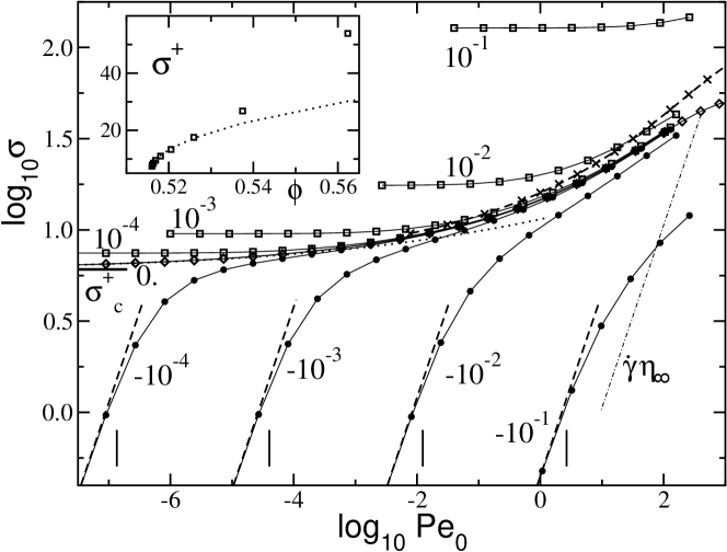
Figure 13: Steady state shear stress $\sigma$ in units of $k_{B}T/d^{3}$ versus Pe${}_{0}=\dot{\gamma}d^{2}/D_{0}$, for the ISHSM at various distances from its glass transition, $\phi-\phi_{c}$ as labeled; circles correspond to fluid, diamonds to the critical, and squares to glassy densities; from Ref. Fuc:03 , where the additional lines are discussed. For the fluid cases, $\phi<\phi_{c}$, dashed lines indicate Newtonian fluid behavior, $\sigma=\eta\dot{\gamma}$, while vertical bars mark Pe$=\dot{\gamma}\tau=1$, with the structural relaxation time taken from $\Phi_{q=7/d}(t=\tau)=0.1$. The additional stress which would arise from the background solvent viscosity, $\sigma=\dot{\gamma}\eta_{\infty}$, is marked by a dot-dashed line. For the critical density, $\phi_{c}$, the critical yield stress, $\sigma^{+}_{c}=6.04$, is shown by a horizontal bar. The inset shows the rise of the dynamical yield stress $\sigma^{+}=\sigma(\varepsilon\geq 0,\dot{\gamma}\to 0+)$ in the glass together with a fitted power-law asymptote, $\sigma^{+}=\sigma_{c}^{+}+112\sqrt{\phi-\phi_{c}}$.

As discussed in Section 4, in the fluid, MCT-ITT finds a linear or Newtonian regime in the limit $\dot{\gamma}\to 0$, where it recovers the standard MCT approximation for Newtonian viscosity $\eta_{0}$ of a viscoelastic fluid Goe:91 ; Goe:92 . Hence $\sigma\to\dot{\gamma}\,\eta_{0}$ holds for Pe $\ll 1$, as shown in Fig. 13, where Pe calculated with the structural relaxation time $\tau$ is included. As discussed, the growth of $\tau$ (asymptotically) dominates all transport coefficients of the colloidal suspension and causes an proportional increase in the viscosity $\eta$. For Pe $>1$, the non-linear viscosity shear thins, and $\sigma$ increases sublinearly with $\dot{\gamma}$. The stress versus strain rate plot in Fig. 13 clearly exhibits a broad crossover between the linear Newtonian and a much weaker (asymptotically) $\dot{\gamma}$-independent variation of the stress. In the fluid, the flow curve takes a S-shape in double logarithmic representation, while in the glass it is bent upward only.

Above the transition, the glass melts for any shear rate. Nonetheless, a finite limiting stress (yield stress) must be overcome in order to maintain the flow of the glass:

$$\sigma(\dot{\gamma},\varepsilon\geq 0)\geq\sigma^{+}(\varepsilon\geq 0)=\lim_{\dot{\gamma}\to 0}\sigma(\dot{\gamma},\varepsilon>0)\;.$$

For $\varepsilon\geq 0$ and $\dot{\gamma}\to 0$, the time $\tau^{(\dot{\gamma})}$ for the final decay , Eq. (26), can become arbitrarily slow compared to the time characterizing the decay onto $f_{q}$. Inserting the scaling functions $\Phi^{+}$ from Eq. (28) into the expression Eq. (27c) for the stress, the long time contribution separates out. Importantly, the integrands containing the $\Phi^{+}$ functions depend on time only via $\tilde{t}=t/\tau_{\dot{\gamma}}\propto\dot{\gamma}t$, so that nontrivial limits for the stationary stress follow in the limit $\dot{\gamma}\to 0$. In the ISHSM for $\varepsilon\geq 0$, the yield stress is given by:

$$\sigma^{+}=\frac{k_{B}T\,\tilde{\dot{\gamma}}}{60\pi^{2}}\;\int_{0}^{\infty}\!\!d\tilde{t}\,\int\!\!dk\;k^{5}\;\frac{S^{\prime}_{k}S^{\prime}_{\breve{k}(\tilde{t})}}{\breve{k}(\tilde{t})\,S^{2}_{k}}\;\left(\Phi^{+}_{\breve{k}(\tilde{t})}(\tilde{t})\right)^{2}\;,$$ (28d)

The existence of a dynamic yield stress in the glass phase is thus seen to arise from the scaling law in Eq. (28), which is clearly borne out in the Figs. 11 and 12. The yield stress arises from those fluctuations which require the presence of shearing to prevent their arrest. Even though $\sigma^{+}$ requires the solution of dynamical equations, in MCT-ITT it is completely determined by the equilibrium structure factor $S_{q}$. This may suggest a connection of MCT to the potential energy paradigm for glasses, as recently discussed Angelani00 ; Broderix00 . One might argue that $\sigma^{+}$ arises because the external driving allows the system to overcome energy barriers so that different metastable states can be reached. This interpretation would agree with ideas from spin-glass Ber:00 and soft-glassy rheology Sol:97 ; Sol:98 ; Fie:00 . MCT-ITT indicates how shear achieves this in the case of colloidal suspensions. It pushes fluctuations to shorter wavelengths where smaller particle rearrangements cause their decorrelation.

The increase of the amplitude of the yielding master functions $\Phi^{+}$ in Eq. (28) originates in the increase of the arrested structure in the unsheared glass Eq. (25). In consequence the yield stress should rapidly increase as one moves further into the glass phase $\sigma^{+}-\sigma^{+}_{c}\propto\sqrt{\varepsilon}$ should (approximately) hold; see however Haj:09 for the more complicated rigorous expression. Indeed, the inset of Fig. 12 shows a good fit of this anomalous increase to the numerical data. It is one of the hallmarks of the weakening of the glass upon approaching the glass transition from the low temperature or high density side.

5.2 Schematic $F_{12}^{(\dot{\gamma})}$-model

The universal aspects described in the previous Section 4 are contained in any ITT model that contains the central bifurcation scenario and recovers Eqs. (20,22). Equation (20) states that spatial and temporal dependences decouple in the intermediate time window. Thus it is possible to investigate ITT models without proper spatial resolution. Because of the technical difficulty to evaluate the anisotropic functionals in Eqs. (11d,14), it is useful to restrict the description to few or to a single transient correlator. The best studied version of such a one-correlator model is the $F_{12}^{(\dot{\gamma})}$-model.

5.2.1 Definition and parameters

In the schematic $F_{12}^{(\dot{\gamma})}$-model Fuc:03 a single ’typical’ density correlator $\Phi(t)$, conveniently normalized according to $\Phi(t\to 0)=1-\Gamma t$, obeys a Zwanzig-Mori memory equation which is modeled according to Eq. (13)

$$\partial_{t}\Phi(t)+\Gamma\left\{\Phi(t)+\int_{0}^{t}dt^{\prime}\;m(t-t^{\prime})\;\partial_{t^{\prime}}\Phi(t^{\prime})\right\}=0\;.$$ (29a)

The parameter $$\Gamma F_{12}^{(\dot{\gamma})} \lambda$$ mimics the short time, microscopic dynamics, and depends on structural and hydrodynamic correlations. The memory function describes stress fluctuations which become more sluggish together with density fluctuations, because slow structural rearrangements dominate all quantities. A self consistent approximation closing the equations of motion is made mimicking Eq. (14a). In the -model one includes a linear term (absent in Eq. (14a)) in order to sweep out the full range of values in Eq. (21), and in order to retain algebraic simplicity:

$$m(t)=\frac{v_{1}\,\Phi(t)+v_{2}\,\Phi^{2}(t)}{1+\left(\dot{\gamma}t/\gamma_{c}\right)^{2}}$$ (29b)

This model, for the quiescent case $\dot{\gamma}=0$, was introduced by Götze in 1984 Goe:84 ; Goe:91 and describes the development of slow structural relaxation upon increasing the coupling vertices $v_{i}\geq 0$; they mimic the dependence of the vertices in Eq. (14) at $\dot{\gamma}=0$ on the equilibrium structure given by $S_{q}$. Under shear an explicit time dependence of the couplings in $m(t)$ captures the decorrelation by shear in Eq. (14). The parameter $\gamma_{c}$ sets a scale that is required in order for the accumulated strain $\dot{\gamma}t$ to matter. Shearing causes the dynamics to decay for long times, because fluctuations are advected to smaller wavelengths where small scale Brownian motion relaxes them. Equations (29a,29b) lead, with $\Phi(t)=f^{c}+(1-f^{c})^{2}\,{\cal G}(t,\varepsilon,\dot{\gamma})$, and the choice of the vertices $v_{2}=v_{2}^{c}=2$, and $v_{1}=v_{1}^{c}+\varepsilon\,(1-f^{c})/f^{c}$, where $v_{1}^{c}=0.828$, to the critical glass form factor $f^{c}=0.293$ and to the stability equation (22), with parameters

$$\lambda=0.707\,,\;c^{(\dot{\gamma})}=0.586/\gamma_{c}^{2}\,\mbox{, and }\;t_{0}=0.426/\Gamma\;.$$

The $F_{12}^{(\dot{\gamma})}$-model possesses a line of glass transitions where the long time limit $f=\Phi(t\to\infty)$ jumps discontinuously; it obeys the equivalent equation to Eq. (21). The glass transition line is parameterized by $(v_{1}^{c},v_{2}^{c})=((2\lambda-1),1)/\lambda^{2}$ with $0.5\leq\lambda<1$, and $f^{c}=1-\lambda$. The present choice of transition point $(v_{1}^{c},v_{2}^{c})$ is a typical one, which corresponds to the given typical $\lambda$-value. The separation parameter $\varepsilon$ is the crucial control parameter as it takes the system through the transition.

For simplicity, the quadratic dependence of the generalized shear modulus on density fluctuations is retained from the microscopic Eq. (11d). It simplifies because only one density mode is considered, and as, for simplicity, a dependence of the vertex (prefactor) $v_{\sigma}$ on shear is neglected

$$g(t,\dot{\gamma})=v_{\sigma}\,\Phi^{2}(t)+\eta_{\infty}\;\delta(t-0+)\;.$$ (29c)

The parameter $\eta_{\infty}$ characterizes a short-time, high frequency viscosity and models viscous processes which require no structural relaxation, like in the general case Eq. (15). Together with $\Gamma$, it is the only model parameter affected by HI. Steady state shear stress under constant shearing, and viscosity then follow via integrating up the generalized modulus:

$$\sigma=\eta\;\dot{\gamma}=\dot{\gamma}\;\int_{0}^{\infty}\!\!\!dt\;g(t)=\dot{\gamma}\;\int_{0}^{\infty}\!\!\!dt\;v_{\sigma}\Phi^{2}(t)+\dot{\gamma}\;\eta_{\infty}\;.$$ (30)

Also, when setting shear rate $\dot{\gamma}=0$ in Eqs. (29a,29b), so that the schematic correlator belongs to the quiescent, equilibrium system, the frequency dependent moduli are obtained from Fourier transforming:

$$G^{\prime}(\omega)+i\,G^{\prime\prime}(\omega)=i\,\omega\,\int_{0}^{\infty}dt\;e^{-i\,\omega\,t}\;v_{\sigma}\left.\Phi^{2}(t)\right|_{\dot{\gamma}=0}+i\omega\,\eta_{\infty}\;.$$ (31)

Because of the vanishing of the Fourier-integral in Eq. (31) for high frequencies, the parameter $\eta_{\infty}$ can be identified as high frequency viscosity:

$$\lim_{\omega\to\infty}G^{\prime\prime}(\omega)/\omega=\eta^{\omega}_{\infty}\quad,\;\mbox{with }\;\eta^{\omega}_{\infty}=\eta_{\infty}\;.$$ (32)

At high shear, on the other hand, Eq. (29b) leads to a vanishing of $m(t)$, and Eq. (29a) gives an exponential decay of the transient correlator, $\Phi(t)\to e^{-\Gamma\,t}$ for $\dot{\gamma}\to 0$. The high shear viscosity thus becomes

$$\eta^{\dot{\gamma}}_{\infty}=\lim_{\dot{\gamma}\to\infty}\sigma(\dot{\gamma})/\dot{\gamma}=\eta_{\infty}+\frac{v_{\sigma}}{2\,\Gamma}=\eta^{\omega}_{\infty}+\frac{v_{\sigma}}{2\,\Gamma}\;.$$ (33)

5.2.2 Correlators and stability analysis

Representative solutions of the F${}_{12}^{(\dot{\gamma})}$-model are summarized in Fig.9, which bring out the discussed universal aspects included in all ITT models.

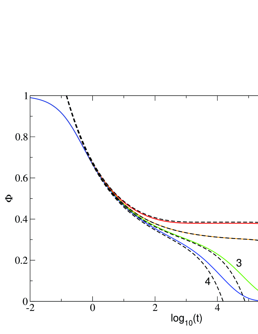
Figure 14: Numerically obtained transient correlators $\Phi\left(t\right)$ (solid lines) for $\varepsilon=0.01$ (red, 1), $\varepsilon=0$ (orange, 2), $\varepsilon=-0.005$ (green, 3) and $\varepsilon=-0.01$ (blue, 4) for the $F_{12}^{(\dot{\gamma})}$-model from Ref. Haj:09 . All curves were calculated with $\dot{\gamma}=10^{-7}$. The dashed lines show the corresponding numerically obtained functions $f_{c}+\left(1-f_{c}\right)^{2}\mathcal{G}\left(t\right)$.

For small separation parameters and shear rates the correlators develop a stretched dynamics located around the critical plateau value $f_{c}$, according to Eqs. (20) to (22). The discussion of the dynamics around this plateau was topic of Section 4. Figure 14 shows these aspects in the $F_{12}^{(\dot{\gamma})}$-model and presents typical correlators and the corresponding $\beta$-correlators. The latter describe how the glassy structure, which is present on intermediate times, is molten either because the density is too low, or the temperature too high, or, alternatively, because of the effect of shearing. For long times $\mathcal{G}\left(t\right)$ merges into the linear asymptote $-t/\tau_{\dot{\gamma}}$ from Eq. (26). In the liquid region, for short times $\mathcal{G}\left(t\right)$ follows $\left(t/t_{0}\right)^{-a}$ from Eq. (22b) and merges into the second power law $-\left(t/\tau_{0}\right)^{b}$ from Eq. (23) for intermediate times with the von MCT Schweidler exponent Goe:91 . In the transition region close to $\varepsilon=0$, after following $\left(t/t_{0}\right)^{-a}$ the function $\mathcal{G}\left(t\right)$ merges directly into the long time asymptote $-t/\tau_{\dot{\gamma}}$. In the yielding glass region, $\mathcal{G}\left(t\right)$ follows $\left(t/t_{0}\right)^{-a}$, arrests on the plateau value $\sqrt{\varepsilon/\left(1-\lambda\right)}$ for intermediate times and merges into the linear asymptote $-t/\tau_{\dot{\gamma}}$ only for long times. So we can summarize that the short- and long time asymptotes are common for all $\varepsilon$ if $\dot{\gamma}\neq 0$ is common. Fig. 15 shows an overview of the properties of $\mathcal{G}\left(t\right)$.

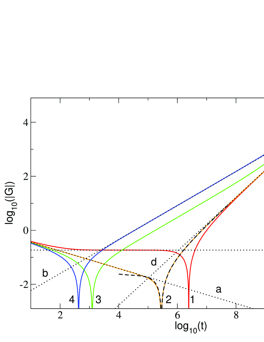
Figure 15: An overview of the properties of $\mathcal{G}\left(t\right)$ (solid lines) for the same values for $\varepsilon$ and $\dot{\gamma}$ as in Fig. 14; from Ref. Haj:09 . The dotted lines show the leading asymptotes for the corresponding time scales: The critical decay $\left(t/t_{0}\right)^{-a}$ (a), the von Schweidler law $-\left(t/\tau_{0}\right)^{b}$ (b), the arrest on the plateau value $\sqrt{\varepsilon/\left(1-\lambda\right)}$ (c) and the shear-induced linear asymptote $-t/\tau_{\dot{\gamma}}$ (d). The dashed line shows a generalization of the latter law evaluated to higher order with a fitted parameter $a_{1}=-1.39\cdot 10^{3}$ (at $\varepsilon=0$).

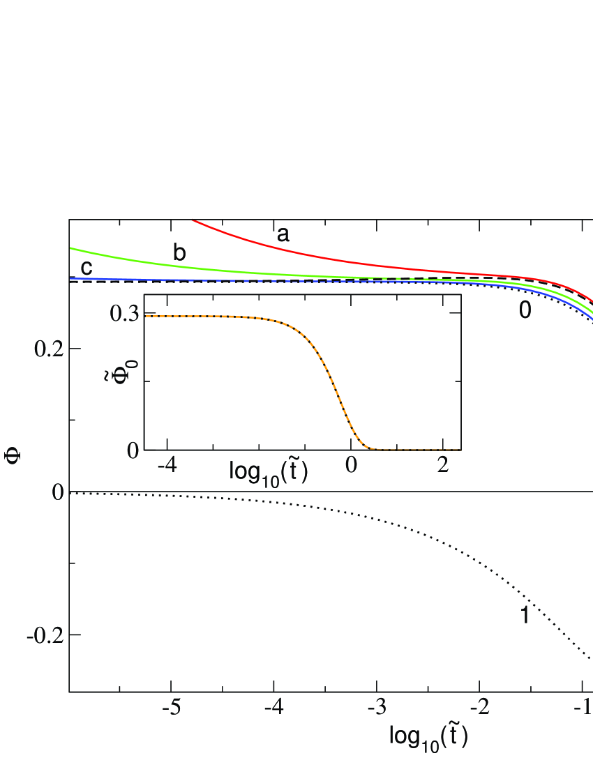
Figure 16: The numerically determined master function of the yielding-process obeying a ’time-shear-superposition principle’ (dotted line) $\Phi^{+}(\tilde{t})=\tilde{\Phi}_{0}\left(\tilde{t}\right)$ (label 0); from Ref. Haj:09 . The solid lines show numerically obtained transient density correlators for $\varepsilon=0$ and $\dot{\gamma}=10^{-7}$ (red, a), $\dot{\gamma}=10^{-9}$ (green, b) and $\dot{\gamma}=10^{-12}$ (blue, c), plotted as functions of the rescaled time $\tilde{t}$. The plots demonstrate that the rescaled correlators converge to the yield master function $\tilde{\Phi}_{0}\left(\tilde{t}\right)$ from the analog of Eq. (28) in the $F_{12}^{(\dot{\gamma})}$-model for $\dot{\gamma}\rightarrow 0$, the blue curve (c) is already quite close to the master curve (0). The dashed line shows $\tilde{\Phi}_{0}\left(\tilde{t}\right)+a_{1}\left|\dot{\gamma}\right|^{c}\tilde{\Phi}_{1}\left(\tilde{t}\right)$ for $\dot{\gamma}=10^{-7}$ and the same numerical value for $a_{1}$ as in Fig. 15, using the leading correction $\tilde{\Phi}_{1}\left(\tilde{t}\right)$ (1), which is shown in the lower panel. This first order expansion already describes quite well the shear-induced decay of the red curve (a). The inset demonstrates that the master function $\tilde{\Phi}_{0}\left(\tilde{t}\right)$ (dotted line) can be well approximated by an exponential function (solid line); the curves overlap completely.

The present $\beta$-scaling law bears some similarity to the one presented by Götze and Sjögren for the description of thermally activated processes in glasses Goe:87 ; Hil:92 . In both cases, ideal glass states are destroyed by additional decay mechanisms. Yet, the ITT equations and the generalised MCT equations differ qualitatively in the mechanism melting the glass. The similarity between both scaling laws thus underlines the universality of the glass stability analysis, which is determined by quite fundamental principles. In Eq. (22), the shear rate can only be a relevant perturbation (at long times) if it appears multiplied by time itself. Symmetry dictates the appearance of $(\dot{\gamma}t)^{2}$, because the sign of the shear rate must not matter. The aspect that shear melts the glass determines the negative sign of $(\dot{\gamma}t)^{2}$.

The melting of the glassy structure during the yield process of Eq. (28) can be explicitly evaluated in the schematic $F_{12}^{(\dot{\gamma})}$-model at $\varepsilon=0$. The yield master function does not depend on $\dot{\gamma}$, and while its form is model-dependent, its initial decay follows from the universal stability equation Eq. (22). Figure 16 shows numerical results, which can be well approximated by an exponential function.

The qualitative agreement between the transient correlators of the ISHSM and the schematic $F_{12}^{(\dot{\gamma})}$-model support the simplification to disregard the spatial structure. The only cost to be paid, is the fixed plateau value $f_{c}$, which can be varied with wavevector in the ISHSM, but not in the schematic model.

5.2.3 Asymptotic laws of flow curves

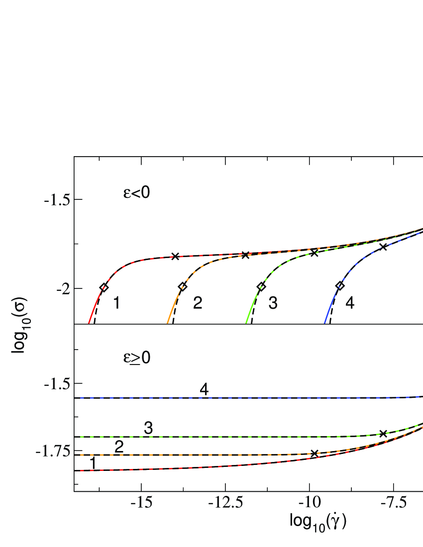
Figure 17: Overview of the numerically obtained flow curves (solid lines) and the asymptotic $\Lambda$-formula evaluated numerically (dashed lines); from Ref. Haj:09 . The liquid curves in the upper panel are shown for $\varepsilon=-10^{-7}$ (red, 1), $\varepsilon=-10^{-6}$ (orange, 2), $\varepsilon=-10^{-5}$ (green, 3) and $\varepsilon=-10^{-4}$ (blue, 4). The lower panel shows the glassy curves for $\varepsilon=0$ (red, 1), $\varepsilon=10^{-5}$ (orange, 2), $\varepsilon=10^{-4}$ (green, 3) and $\varepsilon=10^{-3}$ (blue, 4). Crosses mark the points with $\left|\varepsilon\right|=\varepsilon_{\dot{\gamma}}=\left|\dot{\gamma}t_{0}\right|^{\frac{2a}{1+a}}$. The natural upper boundary for the shear rate, $\dot{\gamma}_{*}$, where the range of validity of the $\Lambda$-formula is left, is also indicated. For $\varepsilon<0$, the natural lower limits for the shear rates, below which the $\Lambda$-formula does not describe the flow curves, are marked by diamonds.

A major advantage of the simplified $F_{12}^{(\dot{\gamma})}$-model is that it allows for asymptotic expansions that qualitatively capture the flow curves. They can thus be investigated in detail addressing such questions as e.g. for the existence of power-law shear thinning Larson , or the dependence of the yield stress on separation parameter. Fig. 17 shows an overview of the numerically obtained flow curves and the corresponding asymptotic results given by the so-called $\Lambda$-formula. While the glass flow curves exhibit an upward curvature only, the fluid curves show a characteristic S-shape, where the initial downward curvature changes to an upward one for increasing shear rate. Both behaviors are captured by the asymptotic expansions. For positive separation parameters the range of validity of the $\Lambda$-formula is given by $\left|\varepsilon\right|\ll 1$ and $\left|\dot{\gamma}t_{0}\right|\ll 1$. These two requirements ensure that $\mathcal{G}\left(t\right)$ describes the dynamics of $\Phi\left(t\right)$ with a sufficiently high accuracy; see Figs. 14 and 15. For sufficiently small negative separation parameters the $\Lambda$-formula is valid in finite shear rate windows only, as it does not reproduce the linear asymptotes for low shear rates. Precise criteria for the range of its validity are known Haj:09 , and Fig. 17 presents an overview of the flow curves and their asymptotic laws.

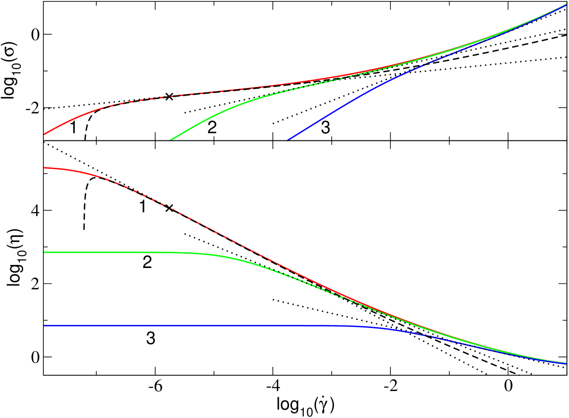
Figure 18: The upper panel shows numerically obtained flow curves (solid lines) for $\varepsilon=-10^{-3}$ (red, 1), $\varepsilon=-10^{-2}$ (green, 2) and $\varepsilon=-10^{-1}$ (blue, 3). The dotted lines show the corresponding inflection tangents, with exponents $p=0.16$, $0.35$, and $0.63$ from left to right. The dashed line shows the numerically evaluated $\Lambda$-formula for $\varepsilon=-10^{-3}$. The shear rate with $\varepsilon=-\varepsilon_{\dot{\gamma}}$ is marked by a cross. The lower panel shows the corresponding results for the viscosity; from Ref. Haj:09 .

While the detailed discussion of the flow curves and their asymptotics leads beyond the present review, see Ref. Haj:09 , the important conclusions from Fig. 17 in the present context are: that the universal aspects discussed in Sect. 4 are recovered, that qualitative agreement is obtained with the results of the ISHSM, and that analytical expressions for the flow curves can be obtained. For example, the critical flow curve follows a generalized Herschel-Bulkley law:

$$\sigma\left(\varepsilon=0,\dot{\gamma}\right)=\sigma_{c}^{+}\sum_{n=0}^{3}\;c_{n}\left|\dot{\gamma}/\dot{\gamma}_{*}\right|^{mn}\;,$$

where $\sigma_{c}^{+}$ is the critical dynamic yield stress and $\dot{\gamma}_{*}$ defines a natural scale for the shear rates in the asymptotic expansion; the upper limit $3$ of the summation is discussed in Ref. Haj:09 . At the transition, this law describes the flow curve correctly for sufficiently small shear rates, see Fig. 17. This result also implies a generalized power-law weakening of the yield stress $\sigma^{+}(\varepsilon)$ when approaching the glass transition for $\varepsilon\searrow 0+$, which is shown in the inset of Fig. 13. In fluid states for $\varepsilon<0$, the flow curves in double logarithmic presentation, viz.  $\log_{10}\left(\sigma\right)$ as function of $\log_{10}\left(\dot{\gamma}\right)$, show an inflection point defined by

$$\frac{d^{2}\left(\log_{10}\left(\sigma\right)\right)}{d\left(\log_{10}\left(\dot{\gamma}\right)\right)^{2}}=0\;.$$

But then in some finite shear rate windows the flow curves can be approximated by the corresponding inflection tangents. The slopes $p$ of the inflection tangents can be interpreted as exponents occurring in some pseudo power laws:

$$\sigma\propto\dot{\gamma}^{p}\;,\quad\Leftrightarrow\quad\eta\propto\dot{\gamma}^{p-1}\;.$$

Figure 18 shows some examples. The asymptotic formula also describes the neighborhood of the inflection point correctly for sufficiently small $\varepsilon$, but does not represent a real power law. In the framework of asymptotic expansions, there is thus no real exponent $p$. The power-law shear thinning often reported in the literature, in the ITT-flow curves thus is a trivial artifact of the double logarithmic plot. Rather, the flow curves on the fluid side exhibit a characteristic S-shape. While this shape is rather apparent when plotting stress versus shear rate, plotting the same data as viscosity as function of shear rate hides it, because the vertical axis gets appreciably stretched.

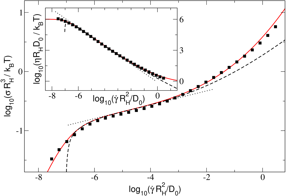
Figure 19: Reduced flow curves for a core-shell dispersion at an effective volume fraction of $\phi_{eff}=0.580$; data from Ref. Sie:09 , analysis from Ref. Haj:09 . Here $R_{H}$ denotes the hydrodynamic radius and $D_{0}$ the self diffusion coefficient of the colloidal particles; $k_{B}T$ is the thermal energy. The solid line (red) shows the result for the fitted $F_{12}^{\left(\dot{\gamma}\right)}$-model with $v_{2}^{c}=2.0$. The fitted parameters are: $\varepsilon=-0.00042$, $\gamma_{c}=0.14$, $v_{\sigma}=70k_{B}T/R_{H}^{3}$, $\Gamma=80D_{0}/R_{H}^{2}$ and $\eta_{\infty}=0.394k_{B}T/R_{H}D_{0}$. The dashed line shows the corresponding result for the $\Lambda$-formula. The dotted line shows the inflection tangent of the numerically determined flow curve with a slope of $p=0.12$. The inset shows the corresponding results for the viscosity.

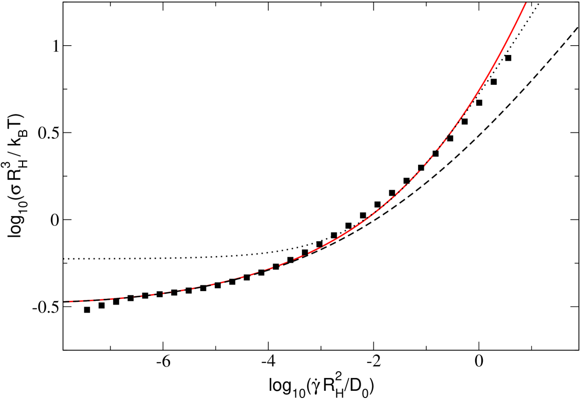
Figure 20: Reduced flow curves for a core-shell dispersion at an effective volume fraction of $\phi_{eff}=0.629$; quantities as defined in the caption of Fig. 19. The solid line (red) shows the result for the fitted $F_{12}^{\left(\dot{\gamma}\right)}$-model with $v_{2}^{c}=2.0$. The fitted parameters are: $\varepsilon=0.000021$, $\gamma_{c}=0.16$, $v_{\sigma}=115k_{B}T/R_{H}^{3}$, $\Gamma=120D_{0}/R_{H}^{2}$ and $\eta_{\infty}=0.431k_{B}T/R_{H}D_{0}$. The dashed line shows the corresponding result for the $\Lambda$-formula. The dotted line shows the fitted Herschel-Bulkley law given by Eq. (34) with the analytically calculated exponent $\tilde{m}=0.489$; data from Ref. Sie:09 , analysis from Ref. Haj:09 .

5.2.4 Test of asymptotics in a polydisperse dispersion

While the asymptotic expansions in the previous section provide an understanding of the contents of the MCT-ITT scenario, experimental tests of the asymptotic laws require flow curves over appreciable windows in shear rate.

Figure 19 and Fig. 20 show experimental data recently obtained by Siebenbürger et al. Sie:09 on polydisperse dispersions of the thermosensitive core-shell particles introduced in Sect. 3.1.2 Cra:06 . In all cases stationary states were achieved after shearing long enough, proving that ageing could be neglected even for glassy states. Because of the appreciable poyldispersity in particle size (standard deviation 17 %) crystallization could efficiently be prevented and flow curves over extremely wide windows could be obtained. Two flow curves from their work can be used to test the asymptotic results.

Fig. 19 shows the result for a liquid-like flow curve where the asymptotic $\Lambda$-formula holds for approximately four decades. The pseudo power law resulting from the inflection tangent of the flow curve holds for approximately two decades within the range of validity of the $\Lambda$-formula.

Fig. 20 shows the result for a flow curve, where a small positive separation parameter was necessary to fit the flow curve and the linear viscoelastic moduli simultaneously. The data are compatible with the (ideal) concept of a yield stress, but fall below the fit curves for very small shear rates. This indicates the existence of an additional decay mechanism neglected in the present approach Cra:08 ; Sie:09 . Again, the $\Lambda$-formula describes the experimental data correctly for approximately four decades. For higher shear rates, an effective Herschel-Bulkley law

$$\sigma(\dot{\gamma}_{*}\ll\left|\dot{\gamma}\right|\ll\Gamma,\varepsilon=0)=\tilde{\sigma}_{0}+\tilde{\sigma}_{1}\left|\dot{\gamma}t_{0}\right|^{\tilde{m}}$$ (34)

with constant amplitudes and exponent $\tilde{m}=0.49$ can be fitted in a window of approximately two decades. The constant $\tilde{\sigma}_{0}$ is not the actual yield stress, $\sigma^{+}$, which is obtained in the limit of vanishing shear rate, $\sigma^{+}=\sigma(\dot{\gamma}\to 0)$, but is larger,

The experimental data of the polydisperse samples, which exhibit structural dynamics over large windows, and their fits with the full schematic model, will be taken up again in Sect. 6.2, where additionally the linear response moduli are considered, as had been done Sect. 3.1.2 for the less polydisperse samples affected by crystallization.

6 Comparison of theory and experiment

As MCT-ITT contains uncontrolled approximations, justification to studying it, can be obtained only from its power to rationalize experimental observations. Because the transient density fluctuations are the central quantity in the approach, density correlators shall be considered first. Flow curves have been studied in most detail experimentally and in simulations, and thus are considered next.

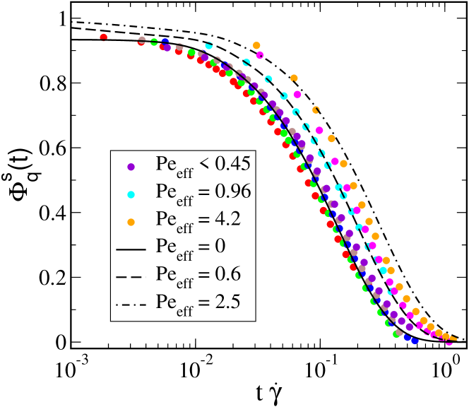
Figure 21: Steady state incoherent intermediate scattering functions $\Phi^{s}_{q}(t)$ as functions of accumulated strain $\dot{\gamma}t$ for various shear rates $\dot{\gamma}$; the data were obtained in a colloidal hard sphere dispersion at packing fraction $\phi=0.62$ (at $\varepsilon\approx 0.07$) using confocal microscopy Bes:07 ; the wavevector points in the vorticity ($\bf\hat{z}$) direction and has $q=3.8/R$ (at the peak of $S_{q}$). The effective Peclet numbers Pe${}_{\rm eff}=4R^{2}\dot{\gamma}/D_{s}$ are estimated with the short time self diffusion coefficient $D_{s}\approx D_{0}/10$ at this concentration Meg:98 . ISHSM calculations with separation parameter $\varepsilon=0.066$ at $qR=3.9$ (PY-$S_{q}$ peaking at $qR=3.5$), and for strain parameter $\gamma_{c}=0.033$, are compared to the data for the Pe_eff values labeled. The yielding master function at Pe${}_{\rm eff}=0$ lies in the data curves which span $0.055\leq$ Pe${}_{\rm eff}\leq 0.45$, but discussion of the apparent systematic trend of the experimental data would require ISHSM to better approximate the shape of the final relaxation process; from Ref. Fuc:09 .

6.1 ISHSM and single particle motion under steady shear

Detailed measurements of the stationary dynamics under shear of a colloidal hard sphere glass have recently been obtained by confocal microscopy Bes:07 . Single particle motion was investigated in a shear-molten glass at roughly the wavevector inverse to the average particle separation. Figure 21 shows self-intermediate scattering functions measured for wavevectors along the vorticity direction where neither affine particle motion nor wavevector advection appears. The stationary correlators deep in the glass, for shear rates spanning almost two decades, are shown as function of accumulated strain $\dot{\gamma}t$, to test whether a simple scaling $\tau_{\dot{\gamma}}\sim 1/\dot{\gamma}$ as predicted by Eq. (28) holds. Small but systematic deviations are apparent which have been interpreted as a power law $\tau_{\dot{\gamma}}\sim\dot{\gamma}^{-0.8}$ Bes:07 ; Sal:08 . ISHSM computations were performed for a nearby wavevector where $S_{q}$ is around unity so that coherent and incoherent correlators may be assumed to be similar Pus:78 . Additionally, for the comparison it was assumed that time dependent transient and stationary fluctuation functions agree. The yielding master function from Eq. (28) in ISHSM can be fitted to the data measured at small effective Peclet numbers Pe_eff, by using for the phenomenological ‘strain rescaling parameter’ $\gamma_{c}=0.033$; the smallness of the fitted value, which would be expected to be of order unity, is not yet understood. The effective Peclet number Pe${}_{\rm eff}=4R^{2}\dot{\gamma}/D_{s}$ with $D_{s}/D_{0}=0.1$ taken from Meg:98 measures the importance of shear relative to the Brownian diffusion time obtained from the short time self diffusion coefficient $D_{s}$ at the relevant volume fraction. At the larger effective Peclet numbers, Pe${}_{\rm eff}\geq 0.5$, for which the short-time and final (shear-induced) relaxation processes move closer together, the model gives quite a good account of the $\dot{\gamma}$-dependence.

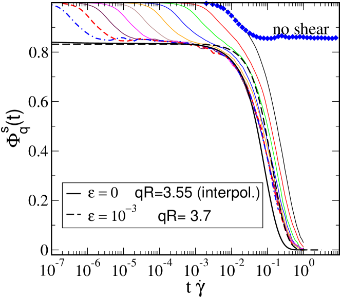
Figure 22: Steady state incoherent intermediate scattering functions $\Phi^{s}_{q}(t)$ measured in the vorticity direction as functions of accumulated strain $\dot{\gamma}t$ for various shear rates $\dot{\gamma}$; data from molecular dynamics simulations of a supercooled binary Lenard-Jones mixture below the glass transition are taken from Ref. Var:06b . These collapse onto a yield scaling function at long times. The wavevector is $q=3.55/R$ (at the peak of $S_{q}$). The quiescent curve, shifted to agree with the one at the highest $\dot{\gamma}$, shows ageing dynamics at longer times outside the plotted window. The apparent yielding master function from simulation is compared to the ones calculated in ISHSM for glassy states at or close to the transition (separation parameters $\varepsilon$ as labeled) and at nearby wave vectors (as labeled). ISHSM curves were chosen to match the plateau value $f_{q}$, while strain parameters $\gamma_{c}=0.083$ at $\varepsilon=0$ (solid line) and $\gamma_{c}=0.116$ at $\varepsilon=10^{-3}$ (dashed line) were used; from Ref. Fuc:09 .

The shape of the final relaxation step in a shear-molten glass can be studied even more closely in recent computer simulations, where a larger separation of short and long time dynamics could be achieved Var:06b . In these molecular dynamics simulations of an undercooled binary Lenard-Jones mixture, schematic ITT models give a good account of the steady state flow curves, $\sigma(\dot{\gamma})$ Var:06 ; Hen:05 ; this will be discussed in Sect. 6.3. Figure 22 shows the corresponding stationary self intermediate scattering functions for a wavevector near the peak in $S_{q}$, oriented along the vorticity direction, for shear rates spanning more than four decades. Collapse onto a master function when plotted as function of accumulated strain is nicely observed as predicted by Eq. (28). At larger shear rates, the correlators raise above the master function; this resembles the behaviour observed in the confocal experiments in Fig. 21, and in the theoretical calculations in Figs. 11 and 16. Assuming again that transient coherent correlators can be fitted to stationary incoherent ones, the shape of the master function can be fitted with the ISHSM, using again an unaccountedly small strain parameter $\gamma_{c}$ . After this rescaling, modest but visible differences in the shapes remain: the theoretical master function decays more steeply than the one from simulations.

Overall, theory and experiment agree in finding a two step relaxation process, where shear has a strong effect on the final structural relaxation, while the short time diffusion is not much affected. This supports the central MCT-ITT prediction that shearing speeds up the structural rearrangements in a concentrated dispersion close to vitrification. More detailed comparisons await better theoretical calculations where the effect of shear on the stationary density fluctuation functions is taken into account more faithfully than in the ISHSM.

6.2 F${}_{12}^{(\dot{\gamma})}$-model and shear stresses in equilibrium and under flow in a polydisperse dispersion

A central result of MCT-ITT concerns the close connection between structural relaxation at the glass transition and the rheological properties far from equilibrium. The ITT approach aims to unify the understanding of these two phenomena, which were introduced wrt. experimental data in Sects. 3.1.1 and 5.2.4, respectively. MCT-ITT requires, as sole input, information on the equilibrium structure (namely $S_{q}$), and, first gives a formally exact generalization of the shear modulus to finite shear rates, $g(t,\dot{\gamma})$, which is then approximated in a consistent way. A novel dense colloidal dispersion serves as experimental model system, whose linear and nonlinear rheology can be determined over very broad windows of control parameters. The generalized modulus $g(t,\dot{\gamma})$ can thus be investigated as function of shear rate and time (more precisely frequency), and the MCT-ITT approach can be tested excruciatingly. Thermosensitive core-shell particles consisting of a polystyrene core and a crosslinked poly(N-isopropylacrylamide)(PNIPAM) shell were synthesized and their slightly polydisperse dispersions (standard deviation 17 %) characterized in detail Sie:09 ; see Sect. 3.1.1. While their precise structure factor has not been measured yet, the system can be well considered a slightly polydisperse mixture of hard spheres. Because polydispersity prevents crystallization and the lack of attractions prevents demixing and coagulation, this system opens a window on structural relaxation, which can nicely be tuned by changing the effective packing fraction by varying temperature.

Shear stresses measured in non-linear response of the dispersion under strong steady shearing, and frequency dependent shear moduli arising from thermal shear stress fluctuations in the quiescent dispersion were measured and fitted with results from the schematic F${}_{12}^{(\dot{\gamma})}$-model. Some results from the microscopic MCT for the equilibrium moduli were included also; see Fig. 23. The fits with quiescent MCT for (monodisperse) hard spheres using the PY $S_{q}$ support the finding of Sect. 3.1.2 that MCT accounts for the magnitude of the stresses at the glass transition semi-quantitatively. Because of the polydispersity of the samples, which is neglected in the calculations performed according to the presentation in Sect. 3.1.2, somewhat larger rescaling factors $c_{y}$ are required; they are included in Table 1. Also, the critical packing fraction $\phi_{c}$ of the glass transition again is reproduced with some small error. Because of polydispersity, the experimental estimate $\phi^{c}_{\text{eff}}\approx 0.625$ Sie:09 lies somewhat higher than in the (more) monodisperse case Cra:08 , which is as expected Voi:03 .

Figure 23 gives the comparison of the experimental flow curves and the linear response moduli $G^{\prime}$ and $G^{\prime\prime}$ with theory for five given different effective volume fraction $\phi_{\text{eff}}$ adjusted by varying temperature. On the left-hand side the flow curves $\sigma(\dot{\gamma})$ are presented as function of the bare Peclet number Pe${}_{0}=k_{B}T/(6\pi\eta_{s}R_{H}^{3})\,\dot{\gamma}$, on the right-hand side $G^{\prime}$ and $G^{\prime\prime}$ are displayed as the function of the frequency-Peclet or Deborrah number Pe${}_{\omega}=k_{B}T/(6\pi\eta_{s}R_{H}^{3})\,\omega$, calculated with the respective frequency $\omega$. Table 1 gathers the effective volume fractions together with the fit parameters of the $F_{12}^{\dot{\gamma}}$-model. Note that $G^{\prime}$ and $G^{\prime\prime}$ have been obtained over nearly 7 orders of magnitude in frequency, while the flow curves extend over more than eight decades in shear rate.

The generalized shear modulus $g(t,\dot{\gamma})$ of the $F_{12}^{\dot{\gamma}}$-model (cf. eq. 29c) presents the central theoretical quantity used in these fits. Within the schematic model, the vertex prefactor $v_{\sigma}$ is kept as a shear-independent quantity. It can easily be obtained from the stress and modulus magnitudes. Hydrodynamic interactions enter through $\eta_{\infty}$, which can be obtained from measurements done at high frequencies, and through $\Gamma$, which can be obtained via Eq. (33) from measurements done at high shear rates. Given these three parameters, both the shapes of the flow curves as well as the shapes of the moduli $G^{\prime}$ and $G^{\prime\prime}$ may be obtained as function of the two parameters $\varepsilon$ and $\dot{\gamma}/\gamma_{c}$. The former sets the separation to the glass transition and thus (especially) the longest relaxation time, while the latter tunes the effect of the shear flow on the flow curve.

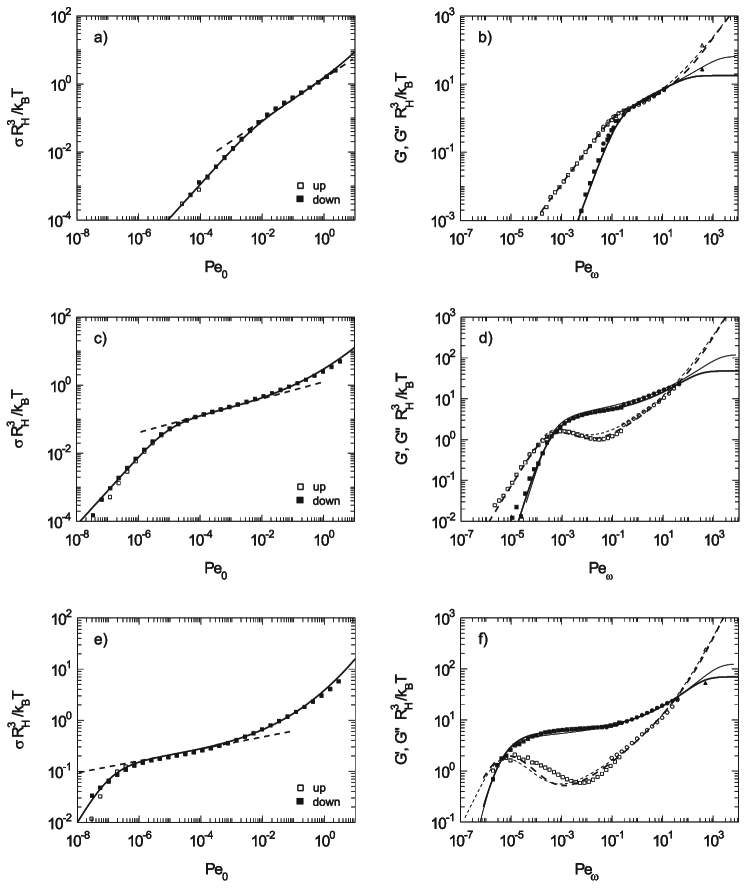
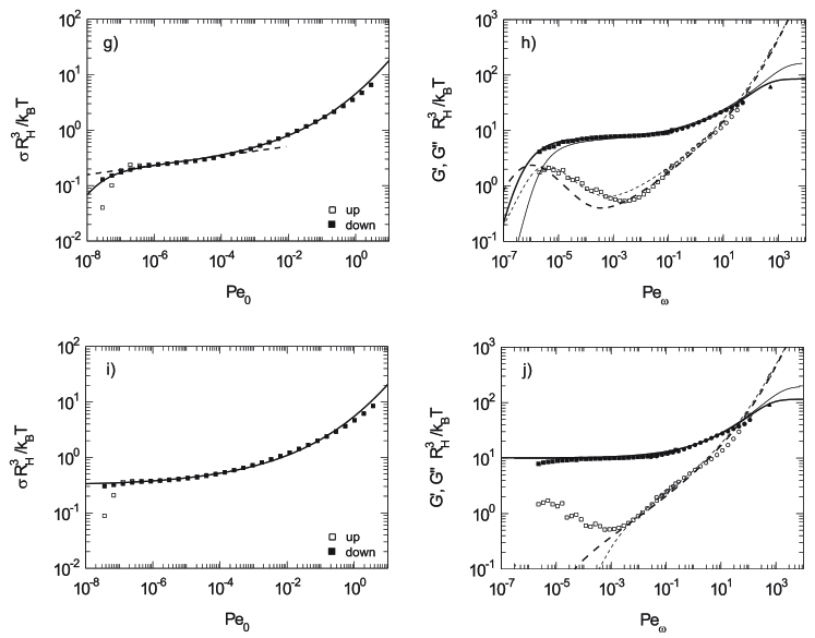
Figure 23: Left column: Reduced flow curves (filled squares) for different volume fractions. The solid lines are the results of the schematic model, the dashed line represent the pseudo power law behaviour; from Ref. Sie:09 .Right column: Reduced frequency dependent moduli for different volume fractions. Full symbols/solid lines represent G’, hollow symbols/dashed lines represent G”. Thick lines are the results of the schematic model, the thin lines the results of the microscopic MCT.Graphs in one row represent the continuous and dynamic measurements at one volume fraction. a and b at $\phi_{\text{eff}}$ = 0.530 , c and d at $\phi_{\text{eff}}$ = 0.595 , e and f at $\phi_{\text{eff}}$ = 0.616 , g and h at $\phi_{\text{eff}}$ = 0.625 , and i and j at $\phi_{\text{eff}}$ = 0.627 .

All measured quantities, namely $\sigma$, $G^{\prime}$, and $G^{\prime\prime}$ were converted to the respective dimensionless quantities by multiplication with $R_{H}^{3}/k_{B}T$ where $R_{H}$ is the hydrodynamic radius at the respective temperature. As already discussed above, the experimental control parameters $\dot{\gamma}$ and $\omega$ also were converted by $6\pi\eta_{s}R_{H}^{3}/k_{B}T$ to the respective Peclet numbers.

$\;\phi_{\text{eff}}\;$	$\varepsilon$	$v_{\sigma}$	$\Gamma$	$\gamma_{c}$	$\eta_{\infty}$	$\varepsilon^{\text{micro}}$	$D_{s}/D_{0}$	$c_{y}$	p
	F${}_{12}^{(\dot{\gamma})}$-mod.	$\left[\frac{k_{B}T}{R_{H}^{3}}\right]$	$\left[\frac{D_{0}}{R_{H}^{2}}\right]$		$\left[\frac{k_{B}T}{D_{0}R_{H}}\right]$	micro.
0.530	-0.072000	18	20	0.0845	0.2250	-0.10	0.3	2.3	0.631
0.595	-0.003500	48	50	0.1195	0.2400	-0.008	0.3	2.3	0.248
0.616	-0.000420	70	80	0.1414	0.3938	-0.001	0.3	2.3	0.117
0.625	-0.000170	85	90	0.1491	0.4250	-0.001	0.3	3.0	0.0852
0.627	0.000021	115	120	0.1622	0.4313	0.002	0.3	3.5	-

Table 1: Packing fraction $\phi_{\text{eff}}$ and parameters $v_{\sigma}$, $\Gamma$, $\gamma_{c}$ and $\eta_{\infty}$ of the fit using the schematic $F_{12}^{\dot{\gamma}}$-model for the measurements shown in Fig. 23; from Ref. Sie:09 . The parameters $\varepsilon$, short time diffusion coefficient $D_{s}/D_{0}$, and rescaling factor $c_{y}$ from the microscopic linear response calculation using MCT , and the pseudo-power law exponent $p$ are included, also.

Evidently, both the reduced moduli, the Pe number, and the packing fraction depend on the effective particle volume $R_{H}^{3}$. In the polydisperse sample, actually a distribution of values $R_{H}^{3}$ exists, whose variance may be determined by disc centrifugation at low concentration, and which is fixed for one given sample. Close to the glass transition the size distribution thus is (almost) density independent, and $R_{H}^{3}(T)$ is the single experimental control parameter, whose small change upon varying temperature $T$ drives the system through the glass transition.

Figure 23 demonstrates that the rheological behavior of a non-crystallizing colloidal dispersion can be modeled in a highly satisfactory manner by five parameters that display only a weak dependence on the effective volume fraction of the particles. Increasing the effective packing fraction drives the system towards the glass transition, viz. $\varepsilon$ increases with $\phi_{\text{eff}}$. Stress magnitudes (measured by $v_{\sigma}$) also increase with $\phi_{\text{eff}}$, as do high frequency and high shear viscosities; their difference determines $\Gamma$. The strain scale $\gamma_{c}$ remains around the reasonable value 10%. In spite of the smooth and small changes of the model parameters, the $F_{12}^{\dot{\gamma}}$-model achieves to capture the qualitative change of the linear and non-linear rheology. The measured Newtonian viscosity increases by a factor around $10^{5}$. The elastic modulus $G^{\prime}$ at low frequencies is utterly negligible at low densities, while it takes a rather constant value around $10k_{B}T/R^{3}_{H}$ at high densities. An analogous observation holds for the steady state shear stress $\sigma(\dot{\gamma})$, which at high densities takes values around $0.3k_{B}T/R^{3}_{H}$ when measured at lowest shear rates. For lower densities, shear rates larger by a factor around $10^{7}$ would be required to obtain such high stress values.

At volume fractions around 0.5 the suspension is Newtonian at small Pe₀. Approaching the glass transition leads to a characteristic S-shape of the flow curves and the Newtonian region becomes more and more restricted to the region of smallest $Pe_{0}$. Concomitantly, a pronounced minimum in $G^{\prime\prime}$ starts to develop, separating the slow structural relaxation process from faster, rather density independent motions, while $G^{\prime}$ exhibits a more and more pronounced plateau. At the highest density (Fig. 23 panels i and j), the theory would conclude that a yielding glass is formed, which exhibits a finite elastic shear modulus (elastic constant) $G_{\infty}=G^{\prime}(\omega\to 0)$, and a finite dynamic yield stress, $\sigma^{+}=\sigma(\dot{\gamma}\to 0)$. The experiment shows, however, that small deviations from this glass like response exist at very small frequencies and strain rates. Description of this ultra-slow process requires extensions of the present MCT-ITT which are discussed in Ref. Cra:08 .

Considering the low frequency spectra in $G^{\prime}(\omega)$ and $G^{\prime\prime}(\omega)$, microscopic MCT and schematic model provide completely equivalent descriptions of the measured data. Differences in the fits in Fig. 23 for Pe${}_{\omega}\leq 1$ only remain because of slightly different choices of the fit parameters which were not tuned to be close. These differences serve to provide some estimate of uncertainties in the fitting procedures. Main conclusion of the comparisons is the agreement of the moduli from microscopic MCT, schematic ITT model, and from the measurements. This observation strongly supports the universality of the glass transition scenario which is a central line of reasoning in the ITT approach to the non-linear rheology.

6.3 F${}_{12}^{(\dot{\gamma})}$-model and flow curves of a simulated supercooled binary liquid

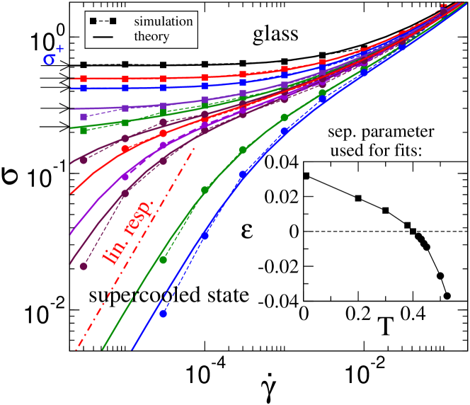
Figure 24: Flow curves $\sigma(\dot{\gamma})$ reaching from the supercooled to the glassy state of a simulated binary LJ mixture. The data points correspond to the temperatures $T=0.525,0.5,0.45,0.44,0.43,0.42,0.4,0.38,0.3,0.2$ and $0.01$ in LJ-units (from bottom to top). $F_{12}^{(\dot{\gamma})}$-model curves fitted by eye are included as lines. The inset shows the relation between the fitted separation parameters and temperature. Units are converted by $\sigma=1.5\sigma_{\rm theo}$ and $\dot{\gamma}=1.3\dot{\gamma}_{\rm theo}\Gamma$; from Hen:05 . The arrows mark the values of the extrapolated dynamic yield stresses $\sigma^{+}(\varepsilon)$.

In large scale molecular dynamics simulations a 80:20 binary mixture of Lennard-Jones (LJ) particles at constant density was supercooled under shear. This model has well known equilibrium properties and many aspects that can be understood consistenly within MCT Kob95 . To account for shearing, it was used together with Lees-Edwards boundary conditions and the SLLOD equations of motion to develop a linear velocity profile. Note that in the simulation solvent effects are obviously lacking, and the simulated flow curves thus provide support for the notion that shear thinning can arise from shear-induced speed up of the structural relaxation; it is evident in Fig. 22. Because the microscopic motion is Newtonian, the theoretical description of this model goes beyond the framework of Sect. 2. Yet the universality of the structural long time dynamics, predicted by MCT Fra:98 and also retained in MCT-ITT, supports to apply MCT-ITT to the simulation data. Moreover, the independence of the glassy dynamics on the employed microscopic motion was explicitly confirmed in simulations of the mixture Gle:98 . This supercooled simple liquid has been characterized quite extensively under shear Ber:02 ; Var:04 ; Var:06 ; Hen:05 ; Var:06b , and thus fits of the flow curves provide challenging tests to the schematic F${}_{12}^{(\dot{\gamma})}$-model.

Figure 25: Dynamic yield stress estimated from the simulations of a supercooled binary LJ mixture under steady shear shown in Fig. 24, and its temperature dependence (in LJ units); from Ref. Var:06 . The estimate uses the stress values for the two lowest simulated shear rates, namely $\dot{\gamma}=10^{-5}$ (triangle) and $\dot{\gamma}=3\times 10^{-6}$ (circle); the extrapolation with the $F_{12}^{(\dot{\gamma})}$-model is shown by diamonds. At temperatures below $T=0.38$, (almost) the same shear stress is obtained for both values of $\dot{\gamma}$ and the extrapolation, indicating the presence of a yield stress plateau.

Figure 24 shows the stress-shear rate dependence as flow curves, ranging from supercooled states to the glassy regime; LJ units are used as described in Var:06 . The solid lines are fits to the simulation data with the $F_{12}^{(\dot{\gamma})}$-model, which reproduce the transition from a shear-thinning fluid to a yielding glass quite well. Coming from high shear rates, the flow curves of the supercooled state pass to the linear response regime in the lower left corner, indicated by a dashed-dotted line with slope 1. On approaching the transition point, the linear response regime shifts to lower and lower shear rates. Beyond the fluid domain, the existence of a dynamic yield stress $\sigma^{+}=\lim_{\dot{\gamma}\to 0}\sigma>0$ is supported by the simulation results, which sustain a stress plateau over three decades in shear rate. Best $F_{12}^{(\dot{\gamma})}$-model fits are obtained for a $T_{c}=0.4$ suggesting a slightly lower transition temperature Flenner05 as determined from the simulations of the quiescent system, where $T_{c}=0.435$ was found Kob95 . The reason may be the ergodicity restoring processes which were also observed in the colloidal experiments shown in Figs. 7, 20, and 23

The stress plateau is best developed for temperatures deep in the glassy phase extending over about two decades in shear rate. Its onset is shifted toward progressively lower $\dot{\gamma}$ as the temperature is increased toward $T_{c}$. This makes an estimate of the dynamic yield stress, $\sigma^{+}(T)\equiv\sigma(T;\dot{\gamma}\to 0)$, a difficult task for temperatures below but close to $T_{c}$. Nevertheless, an estimate of $\sigma^{+}(T)$ is interesting because it highlights the anomalous weakening of the glass when heating to $T_{c}$. Testing the MCT predictions below $T_{c}$ has previously not been possible in simulations because of problems to reach the equilibrated or steady state at sufficiently low shear rates. Figure 25 significantly supports the notion of a glass transition under shear as it presents the first simulations result exibiting the predicted anomalous softening in an elastic property of the glass upon approaching the transition from the glass side, viz. upon heating.

7 Summary and outlook

The present review explored the connection between the physics of the glass transition and the rheology of dense colloidal dispersions, including in strong steady shear flow. A microscopic theoretical approach for the shear-thinning of concentrated suspensions and the yielding of colloidal glasses was presented, which builds on the mode coupling theory (MCT) of idealized glass transitions. The extension to strongly driven stationary states uses the so-called ITT (integration through transients) approach, which leads to a scenario of shear melting a glass, whose universal aspects can be captured in simplified schematic models. Consecutive generalizations of ITT to arbitrary time-dependent states far from equilibrium Bra:07 and to arbitrary flow geometries Bra:08 , have yielded a non-Newtonian constitutive equation applicable to concentrated dispersions in arbitrary homogeneous flows (not reviewed here), albeit still under the approximation that hydrodynamic interactions are neglected. Within the theory, this approximation becomes valid close to the glass transition and for weak but nonlinear flows, where the slow structural relaxation dominates the system properties, and where hydrodynamic interactions only affect the over-all time scale.

The structural dynamics under flow is predicted to result from a competition between local particle hindrance (termed cage effect) and the compression / stretching (i.e. advection) of the wavelength of fluctuations induced by the affine particle motion with the flow. Measurements of the single particle motion in the stationary state under shear support the theoretical picture that shear speeds up the structural dynamics, while instantaneous structural correlations remain rather unaffected. Model dispersions made of thermo-sensitive core-shell particles allow to investigate the close vicinity of the transition. Measurements of the equilibrium stress fluctuations, viz. linear storage and loss moduli, and measurements of flow curves, viz. nonlinear steady state shear stress versus shear rate, for identical external control parameters verify that the glassy structural relaxation can be driven by shearing and in turn itself dominates the low shear or low frequency rheology.

In the employed theoretical approach, the equilibrium structure factor $S_{q}$ captures the particle interactions. Theory misses an ultra-slow decay of all glassy states, and neglects (possible) ageing effects.

Acknowledgment

It is a great pleasure to thank all my colleagues for the enjoyable and fruitful collaboration on this topic. I especially thank Mike Cates for introducing me to rheology, and Matthias Ballauff for his inspiring studies. Kind hospitality in the group of John Brady, where part of this review was written, is gratefully acknowledged. Financial support is acknowledged by the Deutsche Forschungsgemeinschaft in SFB-TR6, SFB 513, IRTG 667, and via grant Fu 309/3.

- (1) R. G. Larson, The Structure and Rheology of Complex Fluids (Oxford University Press, New York, 1999).
- (2) W. Götze and L. Sjögren, Rep. Prog. Phys. 55, 241 (1992).
- (3) W. B. Russel, D. A. Saville, and W. R. Schowalter, Colloidal Dispersions (Cambridge University Press, New York, 1989).
- (4) H. M. Laun, R. Bung, S. Hess, W. Loose, O. Hess, K. Hahn, E. Hädicke, R. Hingmann, F. Schmidt and P. Lindner, J. Rheology 36, 743 (1992).
- (5) J. F. Brady, J. Chem. Phys. 99, 567 (1993).
- (6) P. Sollich, F. Lequeux, P. Hébraud and M.E. Cates, Phys. Rev. Lett. 78, 2020 (1997)
- (7) P. Sollich, Phys. Rev. E 58, 738 (1998).
- (8) S. Fielding, P. Sollich, and M.E. Cates, J. Rheol. 44, 323 (2000)
- (9) L. Berthier, J.-L. Barrat and J. Kurchan, Phys. Rev. E 61, 5464 (2000).
- (10) L. Berthier and J.-L. Barrat, J. Chem. Phys. 116, 6228 (2002).
- (11) P. N. Pusey and W. van Megen, Phys. Rev. Lett. 59, 2083 (1987).
- (12) W. Megen and P. N. Pusey, Phys. Rev. A, Phys. Rev. A 43, 5429 (1991).
- (13) W. van Megen and S. M. Underwood, Phys. Rev. Lett. 70, 2766 (1993).
- (14) W. van Megen and S. M. Underwood, Phys. Rev. E 49, 4206 (1994).
- (15) W. van Megen, T. C. Mortensen, J. Müller, and S. R. Williams, Phys. Rev. E 58, 6073 (1998).
- (16) P. Hébraud, F. Lequeux, J. Munch and D. Pine, Phys. Rev. Lett. 78, 4657 (1997).
- (17) C. Beck, W. Härtl and R. Hempelmann, J. Chem. Phys. 111, 8209 (1999).
- (18) E. Bartsch, T. Eckert, C. Pies and H. Sillescu, J. Non-Cryst. Solids, 802, 307 (2002)
- (19) T. Eckert and E. Bartsch, Faraday Discuss. 123, 51 (2003).
- (20) E. R. Weeks, J. C. Crocker, A. C. Levitt, A. Schofield and D. A. Weitz, Science 287, 627 (2000).
- (21) T. G. Mason and D. A. Weitz, Phys. Rev. Lett. 75, 2770 (1995).
- (22) M. Zackrisson, A. Stradner, P. Schurtenberger and J. Bergenholtz, Phys. Rev. E 73, 011408 (2006).
- (23) H. Senff, W. Richtering, J. Chem. Phys. 111, 1705 (1999).
- (24) H. Senff, W. Richtering, Ch. Norhausen, A. Weiss, M. Ballauff, Langmuir 15, 102 (1999).
- (25) G. Petekidis, D. Vlassopoulos and P. Pusey, Faraday Discuss. 123, 287 (1999).
- (26) G. Petekidis,D Vlassopoulos, and P. N. Pusey, J. Phys.: Condens. Matter 16, S3955 (2004).
- (27) G. Petekidis, A. Moussaid, and P. N. Pusey, Phys. Rev. E 66, 051402 (2002); G. Petekidis, D. Vlassopoulos, and P. N. Pusey, Faraday Disc. 123, 287 (2003).
- (28) K. N Pham, G Petekidis, D Vlassopoulos, S. U Egelhaaf, P. N Pusey, and W. C. K Poon, Europhys. Lett. 75, 624 (2006).
- (29) R. Besseling, Eric R. Weeks, A. B. Schofield and W. C. Poon, Phys. Rev. Lett. 99, 028301 (2007).
- (30) J. J. Crassous, M. Siebenbürger, M. Ballauf, M. Drechsler, O. Henrich and M. Fuchs, J. Chem. Phys. 125, 204906 (2006).
- (31) J. J. Crassous, M. Siebenbürger, M. Ballauf, M. Drechsler, D. Hajnal, O. Henrich and M. Fuchs, J. Chem. Phys. 128, 204902 (2008).
- (32) M. Siebenbürger, M. Fuchs, H. Winter, and M. Ballauf, J. Rheol. submitted (2008).
- (33) T. Phung, J. Brady and G. Bossis, J. Fluid Mech. 313, 181 (1996).
- (34) P. Strating, Phys. Rev. E 59, 2175 (1999).
- (35) B. Doliwa and A. Heuer, Phys. Rev. E 61, 6898 (2000).
- (36) E. H Purnomo, D. van den Ende, J Mellema and F Mugele, Europhys. Lett. 76, 74 (2006).
- (37) W. Götze, in Liquids, Freezing and Glass Transition, edited by J. P. Hansen, D. Levesque, and J. Zinn-Justin, Session LI (1989) of Les Houches Summer Schools of Theoretical Physics, (North-Holland, Amsterdam, 1991), 287.
- (38) W. Götze, J. Phys.: Condens. Matter 11, A1 (1999).
- (39) K. Miyazaki and D.R. Reichman, Phys.Rev.E. 66, 050501 (2002),
- (40) K. Miyazaki, D.R. Reichman and R. Yamamoto, Phys.Rev.E. 70, 011501 (2004).
- (41) V. Kobelev and K. S. Schweizer, Phys. Rev. E 71, 021401 (2005).
- (42) M. Fuchs and M. E. Cates, Phys. Rev. Lett. 89, 248304 (2002).
- (43) M. Fuchs and M. E. Cates, J. Phys.: Condens. Matter 17, S1681 (2005)
- (44) M. Fuchs and M. E. Cates, J. Rheol. in preparation (2009).
- (45) J. K. G. Dhont, An introduction to dynamics of colloids (Elsevier Science, Amsterdam, 1996).
- (46) H. Risken 1989 The Fokker–Planck Equation (Springer, Berlin)
- (47) Dhont, J. K. G.; Briels, W. J Rheologica Acta, 47 (2008), 257 - 281
- (48) J. Bender and N. J. Wagner, J. Rheol. 40, 899 (1996).
- (49) F. Varnik, L. Bocquet, and J. L. Barrat, J. Chem. Phys. 120, 2788 (2004).
- (50) R. Ganapathy and A. K. Sood, Phys. Rev. Lett. 96, 108301 (2006).
- (51) P. Ballesta, R. Besseling, L. Isa, G. Petekidis and W. C. K. Poon, Phys. Rev. Lett. x, xx (2008).
- (52) N.G. Van Kampen, Stochastic Processes in Physics and Chemistry, (North Holland, Amsterdam, 2007)
- (53) D. Forster 1975 Hydrodynamic Fluctuations, Broken Symmetry, and Correlation Functions (WA Benjamin, Reading, MA)
- (54) W. Götze and L. Sjögren, Z. Phys. B 65, 415 (1987).
- (55) J. Schofield and I. Oppenheim, Physica A 187, 210 (1992).
- (56) G. Nägele and J. Bergenholtz, J. Chem. Phys. 108, 9893 (1998)
- (57) K. Miyazaki, H.M. Wyss, D. R. Reichman, D. A. Weitz Europhys. Lett. 75, 915 (2006)
- (58) J.M. Brader, Th. Voigtmann, M.E. Cates, and M. Fuchs, Phys. Rev. Lett. 98, 058301 (2007)
- (59) R. A. Lionberger and W. B. Russel, J. Rheol. 38, 1885 (1994).
- (60) A. Onuki and K. Kawasaki, Ann. Phys. (N.Y.) 121, 456 (1979).
- (61) K. Kawasaki and J. D. Gunton, Phys. Rev. A 8, 2048( 1973).
- (62) A. V. Indrani and S. Ramaswamy, Phys. Rev. E 52, 6492 (1995).
- (63) J. Bergenholtz and M. Fuchs, Phys. Rev. E 59, 5706 (1999).
- (64) Dawson K., Foffi G., Fuchs M., Gotze W., Sciortino F., Sperl M., Tartaglia P., Voigtmann T., Zaccarelli E., Phys. Rev. E 63 (2001) 011401.
- (65) Fabbian L., Götze W., Sciortino F., Tartaglia P., and Thiery F., Phys. Rev. E 59 (1999) R1347–R1350. 1999; Sciortino F., this volume, Sciortino F., Nature Materials 1 (2003) 145–146.
- (66) Pham K. N., Puertas A. M., Bergenholtz J., Egelhaaf S. U., Moussaid A., Pusey P. N., Schofield A. B., Cates M. E., Fuchs M. and Poon W. C. K., Science 296 (2002) 104–106. Poon W. C. K., Pham K. N., Egelhaaf S. U. and Pusey P. N., J. Phys. Cond. Matt. 15 (2003) S269-S275.
- (67) M. Fuchs and M. Ballauff, Colloids Surfaces A 270-271, 232 (2005).
- (68) T. Franosch, M. Fuchs, W. Götze, M. R. Mayr, and A. P. Singh, Phys. Rev. E 55, 7153 (1997).
- (69) M. Fuchs and M. R. Mayr, Phys. Rev. E 60, 5742 (1999).
- (70) T. Franosch, W. Götze, M. R. Mayr, and A. P. Singh, J. Non-Cryst. Solids 235-237, 71 (1998).
- (71) R. Verberg, I.M. de Schepper, M.J. Feigenbaum, E.G.D. Cohen, J. Stat. Phys. 87, 1037 (1997).
- (72) O. Henrich, O. Pfeifroth and M. Fuchs, J. Phys.: Condens. Matter 19, 205132 (2007).
- (73) G. Szamel, J. Chem. Phys. 114 8708 (2001)
- (74) Johnson S J, de Kruif C G, May R P 1988 J. Chem. Phys. 89 5909
- (75) Lionberger R A, Russel W B 2000 Adv. Chem. Phys. 111 399
- (76) M. Fuchs and M. E. Cates, Faraday Disc. 123, 267 (2003).
- (77) F. Varnik and O. Henrich, Phys. Rev. B 73, 174209 (2006)
- (78) L. Angelani, R. D. Leonardo, G. Ruocco, A. Scala, and F. Sciortino, Phys. Rev. Lett. 85, 5356 (2000).
- (79) K. Broderix, K. K. Bhattachrya, A. Cavagna, and Z. Zippelius, Phys. Rev. Lett. 85, 5360 (2000).
- (80) D. Hajnal and M. Fuchs, Eur. Phys. J. E, in print (2009); DOI: 10.1140/epje/i2008-10361-0; also at arXiv:0807.1288
- (81) W. Götze, Z. Phys. B 56, 139 (1984).
- (82) M. Fuchs, W. Götze, S. Hildebrand and A. Latz, J. Phys.: Condens. Matter 4, 7709 (1992).
- (83) E. J. Saltzman, G. Yatsenko, and K. S. Schweizer, J. Phys.: Condens. Matter, 20, 244129 (2008).
- (84) Varnik F 2006 J. Chem. Phys. 125 164514
- (85) M. Fuchs, W. Götze, I. Hofacker, and A. Latz, J. Phys.: Condens. Matter 3, 5047-5071 (1991)
- (86) W. G tze and Th. Voigtmann, Phys. Rev. E 67, 021502 (2003) G. Foffi, W. G tze, F. Sciortino, P. Tartaglia, and Th. Voigtmann, Phys. Rev. Lett. 91, 085701 (2003).
- (87) J. Zausch, J. Horbach, M. Laurati, S. U. Egelhaaf, J. M. Brader, Th. Voigtmann, and M. Fuchs, J. Phys.: Condens. Matt. 20, 404210 (2008).
- (88) P. N. Pusey, J. Phys. A 11, 119 (1978).
- (89) O. Henrich, F. Varnik and M. Fuchs, J. Phys.: Condens. Matter 17, S3625 (2005).
- (90) W. Kob and H. C. Andersen, Phys. Rev. E 51, 4626; 52, 4134 (1995).
- (91) T. Gleim T., W. Kob, and K. Binder K., Phys. Rev. Lett. 81, 4404 (1998).
- (92) E. Flenner and G. Szamel, Phys. Rev. E 72, 011205 (2005)
- (93) J. M. Brader, M. E. Cates, and M. Fuchs, Phys. Rev. Lett. 101, 138301 (2008).