On the Throughput Maximization in Dencentralized Wireless Networks

Abstract

A distributed single-hop wireless network with $K$ links is considered, where the links are partitioned into a fixed number ($M$) of clusters each operating in a subchannel with bandwidth $\frac{W}{M}$. The subchannels are assumed to be orthogonal to each other. A general shadow-fading model, described by parameters $(\alpha,\varpi)$, is considered where $\alpha$ denotes the probability of shadowing and $\varpi$ ($\varpi\leq 1$) represents the average cross-link gains. The main goal of this paper is to find the maximum network throughput in the asymptotic regime of $K\to\infty$, which is achieved by: i) proposing a distributed and non-iterative power allocation strategy, where the objective of each user is to maximize its best estimate (based on its local information, i.e., direct channel gain) of the average network throughput, and ii) choosing the optimum value for $M$. In the first part of the paper, the network throughput is defined as the average sum-rate of the network, which is shown to scale as $\Theta(\log K)$. Moreover, it is proved that in the strong interference scenario, the optimum power allocation strategy for each user is a threshold-based on-off scheme. In the second part, the network throughput is defined as the guaranteed sum-rate, when the outage probability approaches zero. In this scenario, it is demonstrated that the on-off power allocation scheme maximizes the throughput, which scales as $\frac{W}{\alpha\varpi}\log K$. Moreover, the optimum spectrum sharing for maximizing the average sum-rate and the guaranteed sum-rate is achieved at $M=1$.

I Introduction

I-A History

A primary challenge in wireless networks is to use available resources efficiently so that the network throughput is maximized. Throughput maximization in multi-user wireless networks has been addressed from different perspectives; resource allocation [3, 4, 5], scheduling [6], routing by using relay nodes [7], exploiting mobility of the nodes [8] and exploiting channel characteristics (e.g., power decay-versus-distance law [9, 10, 11], geometric pathloss and fading [12, 13, 14]).

Among different resource allocation strategies, power and spectrum allocation have long been regarded as efficient tools to mitigate the interference and improve the network throughput. In recent years, power and spectrum allocation schemes have been extensively studied in cellular and multihop wireless networks [15, 4, 16, 17, 18, 19, 20, 3]. In [19], the authors provide a comprehensive survey in the area of resource allocation, in particular in the context of spectrum assignment. Much of these works rely on centralized and cooperative algorithms. Clearly, centralized resource allocation schemes provide a significant improvement in the network throughput over decentralized (distributed) approaches. However, they require extensive knowledge of the network configuration. In particular, when the number of nodes is large, deploying such centralized schemes may not be practically feasible. Due to significant challenges in using centralized approaches, the attention of the researchers has been drawn to the decentralized resource allocation schemes [21, 22, 23, 24, 25, 26].

In decentralized schemes, the decisions concerning network parameters (e.g., rate and/or power) are made by the individual nodes based on their local information. The local decision parameters that can be used for adjusting the rate are the Signal-to-Interference-plus-Noise Ratio (SINR) and the direct channel gain. Most of the works on decentralized throughput maximization target the SINR parameter by using iterative algorithms [23, 24, 25]. This leads to the use of game theory concepts [27] where the main challenge is the convergence issue. For instance, Etkin et al. [25] develop power and spectrum allocation strategies by using game theory. Under the assumptions of the omniscient nodes and strong interference, the authors show that Frequency-Division Multiplexing (FDM) is the optimal scheme in the sense of throughput maximization. They use an iterative algorithm that converges to the optimum power values. In [24], Huang et al. propose an iterative power control algorithm in an ad hoc wireless network, in which receivers broadcast adjacent channel gains and interference prices to optimize the network throughput. However, this algorithm incurs a great amount of overhead in large wireless networks.

A more practical approach is to rely on the channel gains as local decision parameters and avoid iterative schemes. Motivated by this consideration, we study the throughput maximization of a distributed wireless network with $K$ links, operating in a bandwidth of $W$. To mitigate the interference, the links are partitioned into a fixed number ($M$) of clusters, each operating in a subchannel with bandwidth $\frac{W}{M}$, where the subchannels are orthogonal to each other. Throughput maximization of the underlying network is achieved by proposing a distributed and non-iterative power allocation strategy based on the direct channel gains, and then choosing the optimum value for $M$.

I-B Contributions and Relations to Previous Works

In this paper, we study the throughput maximization of a spatially distributed wireless network with $K$ links, where the sources and their corresponding destinations communicate directly with each other without using relay nodes. Wireless networks using unlicensed spectrum (e.g. Wi-Fi systems based on IEEE 802.11b standard [28]) are a typical example of such networks. The cross-link channel gains are assumed to be Rayleigh-distributed with shadow-fading, described by parameters $(\alpha,\varpi)$, where $\alpha$ denotes the probability of shadowing and $\varpi$ ($\varpi\leq 1$) represents the statistical average of the Rayleigh distribution.

The above configuration differs from the geometric models proposed in [9, 8, 10, 11, 29], in which the signal power decays based on the distance between nodes. Unlike [22, 23, 24, 25] which relies on an iterative algorithm using SINR, we assume that each transmitter adjusts its power solely based on its direct channel gain.

If each user maximizes its rate selfishly, the optimum power allocation strategy for all users is to transmit with full power. This strategy results in excessive interference, degrading the average network throughput. To prevent this undesirable effect, one should consider the negative impact of each user’s power on other links. A reasonable approach for each user is to choose a non-iterative power allocation strategy to maximize its best local estimate of the network throughput.

The network throughput in this paper is defined in two ways: i) average sum-rate and ii) guaranteed sum-rate. It is established that the average sum-rate in the network scales at most as $\Theta(\log K)$ in the asymptotic case of $K\to\infty$. This order is achievable by the distributed threshold-based on-off scheme (i.e., links with a direct channel gain above certain threshold transmit at full power and the rest remain silent). Moreover, in the strong interference scenario, the on-off power allocation scheme is the optimal strategy. In addition, the on-off power allocation scheme is always optimal for maximizing the guaranteed sum-rate in the network, which is shown to scale as $\frac{W}{\alpha\varpi}\log K$. These results are different from the result of [30] where the authors use a similar on-off scheme for $M=1$ and prove its optimality only among all on-off schemes. This work also differs from [31] and [32] in terms of the network model. We use a distributed power allocation strategy in a single-hop network, while [31] and [32] consider an ad hoc network model with random connections and relay nodes.

We optimize the average network throughput in terms of the number of the clusters, $M$. It is proved that the maximum average sum-rate and the guaranteed sum-rate of the network for every value of $\alpha$ and $\varpi$ is achieved at $M=1$. In other words, splitting the bandwidth $W$ into $M$ orthogonal sub-channels does not increase the throughput.

The rest of the paper is organized as follows. In Section II, the network model and objectives are described. The distributed on-off power allocation strategy and the network average sum-rate are presented in Section III. We analyze the network guaranteed sum-rate in Section IV. Finally, in Section V, an overview of the results and some conclusion remarks are presented.

I-C Notations

For any functions $f(n)$ and $g(n)$ [33]:

• $f(n)=O(g(n))$ means that $\lim_{n\to\infty}\Big{|}\frac{f(n)}{g(n)}\Big{|}<\infty$.

• $f(n)=\mathit{o}(g(n))$ means that $\lim_{n\to\infty}\Big{|}\frac{f(n)}{g(n)}\Big{|}=0$.

• $f(n)=\omega(g(n))$ means that $\lim_{n\to\infty}\frac{f(n)}{g(n)}=\infty$.

• $f(n)=\Omega(g(n))$ means that $\lim_{n\to\infty}\frac{f(n)}{g(n)}>0$.

• $f(n)=\Theta(g(n))$ means that $\lim_{n\to\infty}\frac{f(n)}{g(n)}=c$, where $0<c<\infty$.

• $f(n)\sim g(n)$ means that $\lim_{n\to\infty}\frac{f(n)}{g(n)}=1$.

• $f(n)\lesssim g(n)$ means that $\lim_{n\to\infty}\frac{f(n)}{g(n)}\leq 1$.

• $f(n)\approx g(n)$ means that $f(n)$ is approximately equal to $g(n)$, i.e., if we replace $f(n)$ by $g(n)$ in the equations, the results still hold.

Throughout the paper, we use $\log(.)$ as the natural logarithm function and $\mathbb{P}\{.\}$ denotes the probability of the given event. Boldface letters denote vectors; and for a random variable $x$, $\bar{x}$ means $\mathbb{E}[x]$, where $\mathbb{E}[.]$ represents the expectation operator. R​H(.) represents the right hand side of the equations.

II Network Model and Objectives

II-A Network Model

In this work, we consider a single-hop wireless network consisting of $K$ pairs of nodes indexed by $\{1,...,K\}$, operating in bandwidth $W$. All the nodes in the network are assumed to have a single antenna. The links are assumed to be randomly divided into $M$ clusters denoted by $\mathbb{C}_{j}$, $j=1,...,M$ such that the number of links in all clusters are the same. Without loss of generality, we assume that $\mathbb{C}_{j}\triangleq\{(j-1)n+1,...,jn\}$, where $n\triangleq\frac{K}{M}$ denotes the cardinality of the set $\mathbb{C}_{j}$ which is assumed to be known to all users. To eliminate the mutual interference among the clusters, we assume an $M$-dimensional orthogonal coordinate system in which the bandwidth $W$ is split into $M$ disjoint subchannels each with bandwidth $\frac{W}{M}$. It is assumed that the links in $\mathbb{C}_{j}$ operate in subchannel $j$. We also assume that $M$ is fixed, i.e., it does not scale with $K$. The power of Additive White Gaussian Noise (AWGN) at each receiver is $\frac{N_{0}W}{M}$, where $N_{0}$ is the noise power spectral density.

The channel model is assumed to be flat Rayleigh fading with the shadowing effect. The channel gain between transmitter $k$ and receiver $i$ is represented by the random variable $\mathcal{L}_{ki}$. For $k=i$, the direct channel gain is defined as $\mathcal{L}_{ki}\triangleq h_{ii}$ where $h_{ii}$ is exponentially distributed with unit mean (and unit variance). For $k\neq i$, the cross channel gains are defined based on a shadowing model as follows:

$$\mathcal{L}_{ki}\triangleq\left\{\begin{array}[]{ll}\beta_{ki}h_{ki},&\textrm{with probability}~{}~{}~{}~{}\alpha\\ 0,&\textrm{with probability}~{}~{}1-\alpha,\end{array}\right.$$ (3)

where $h_{ki}$’s have the same distribution as $h_{ii}$’s, $0\leq\alpha\leq 1$ is a fixed parameter, and the random variable $\beta_{ki}$, referred to as the shadowing factor, is independent of $h_{ki}$ and satisfies the following conditions:

• $\beta_{\min}\leq\beta_{ki}\leq\beta_{\max}$, where $\beta_{\min}>0$ and $\beta_{\max}$ is finite,

• $\mathbb{E}\big{[}\beta_{ki}\big{]}\triangleq\varpi\leq 1$.

It is also assumed that $\{\mathcal{L}_{ki}\}$ and $\{\beta_{ki}\}$ are mutually independent random variables for different $(k,i)$.

All the channels in the network are assumed to be quasi-static block fading, i.e., the channel gains remain constant during one block and change independently from block to block. In addition, we assume that each transmitter knows its direct channel gain.

We assume a homogeneous network in the sense that all the links have the same configuration and use the same protocol. We denote the transmit power of user $i$ by $p_{i}$, where $p_{i}\in\mathscr{P}\triangleq[0,\textrm{P}_{max}]$. The vector $\textbf{{P}}^{(j)}=(p_{(j-1)n+1},...,p_{jn})$ represents the power vector of the users in $\mathbb{C}_{j}$. Also, $\textbf{{P}}^{(j)}_{-i}$ denotes the vector consisting of elements of $\textbf{{P}}^{(j)}$ other than the $i^{th}$ element, $i\in\mathbb{C}_{j}$. To simplify the notations, we assume that the noise power $\frac{N_{0}W}{M}$ is normalized by $\textrm{P}_{max}$. Therefore, without loss of generality, we assume that $\textrm{P}_{max}=1$. Assuming that the transmitted signals are Gaussian, the interference term seen by link $i\in\mathbb{C}_{j}$ will be Gaussian with power

$$I_{i}=\sum_{\begin{subarray}{c}k\in\mathbb{C}_{j}\\ k\neq i\end{subarray}}\mathcal{L}_{ki}p_{k}.$$ (4)

Due to the orthogonality of the allocated sub-channels, no interference is imposed from links in $\mathbb{C}_{k}$ on links in $\mathbb{C}_{j}$, $k\neq j$. Under these assumptions, the achievable data rate of each link $i\in\mathbb{C}_{j}$ is expressed as

$$R_{i}(\textbf{{P}}^{(j)},\boldsymbol{\mathcal{L}}_{i}^{(j)})=\dfrac{W}{M}\log\left(1+\dfrac{h_{ii}p_{i}}{I_{i}+\frac{N_{0}W}{M}}\right),$$ (5)

where $\boldsymbol{\mathcal{L}}_{i}^{(j)}\triangleq(\mathcal{L}_{((j-1)n+1)i},...,\mathcal{L}_{(jn)i})$. To analyze the performance of the underlying network, we use the following performance metrics:

• Network Average Sum-Rate:

  $$\bar{R}_{ave}\triangleq\mathbb{E}\left[\sum_{j=1}^{M}\sum_{l\in\mathbb{C}_{j}}R_{l}(\textbf{{P}}^{(j)},\boldsymbol{\mathcal{L}}_{l}^{(j)})\right],$$ (6)

  where the expectation is computed with respect to $\boldsymbol{\mathcal{L}}_{l}^{(j)}$. This metric is used when there is no decoding delay constraint, i.e., decoding is performed over arbitrarily large number of blocks.

• Network Guaranteed Sum-Rate:

  $$\bar{R}_{g}\triangleq\sum_{j=1}^{M}\sum_{l\in\mathbb{C}_{j}}\mathbb{E}_{h_{{}_{ll}}}\left[R^{*}(h_{ll})\right],$$ (7)

  in which for all $h_{ll}$, $l\in\mathbb{C}_{j}$, we have

  $$R^{*}(h_{ll})\triangleq\sup\,\,{R(h_{ll})},$$ (8)

  such that

  $$\mathbb{P}\left\{R_{l}(\textbf{{P}}^{(j)},\boldsymbol{\mathcal{L}}_{l}^{(j)})<R(h_{ll})\right\}\rightarrow 0.$$ (9)

  This metric is useful when there exists a stringent decoding delay constraint, i.e, decoding must be performed over each separate block, and a single-layer code is used. In this case, as the transmitter does not have any information about the interference term, an outage event may occur. Network guaranteed throughput is the average sum-rate of the network which is guaranteed for all channel realizations.

II-B Objectives

Part I: Maximizing the network average sum-rate: The main objective of the first part of this paper is to maximize the network average sum-rate when the interference is strong enough, i.e., $\mathbb{E}[I_{i}]=\omega(1)$. This is achieved by:

• Proposing a distributed and non-iterative power allocation strategy, where each user maximizes its best estimate (based on its local information, i.e., direct channel gain) of the average network sum-rate.

• Choosing the optimum value for $M$.

To address this problem, we first define a utility function for link $i\in\mathbb{C}_{j}$ ($j=1,...,M$) that describes the average sum-rate of the links in cluster $\mathbb{C}_{j}$ as follows

$$u_{i}(p_{i},h_{ii})\triangleq\mathbb{E}\left[\sum_{l\in\mathbb{C}_{j}}R_{l}(\textbf{{P}}^{(j)},\boldsymbol{\mathcal{L}}_{l}^{(j)})\right],$$ (10)

where the expectation is computed with respect to $\{\mathcal{L}_{kl}\}_{k,l\in\mathbb{C}_{j}}$ excluding $k=l=i$ (namely $h_{ii}$). As mentioned earlier, $h_{ii}$ is considered as the local (known) information for link $i$, however, all the other gains are unknown to user $i$ which is the reason behind statistical averaging over these parameters in (10). User $i$ selects its power using

$$\hat{p}_{i}=\textrm{arg}~{}\max_{p_{i}\in\mathscr{P}}~{}u_{i}(p_{i},h_{ii}).$$ (11)

It will be shown that when the number of links is large and the interference is strong enough, the optimum power allocation strategy for the optimization problem in (11) is the on-off power scheme. Assuming that the channel gains change independently from block to block, each user updates its on-off decision based on its direct channel gain in each block. Given the optimum power vector $\hat{\textbf{{P}}}^{(j)}=(\hat{p}_{(j-1)n+1},...,\hat{p}_{jn})$ obtained from (11), the network average sum-rate is then computed as (6). Next, we choose the optimum value of $M$ such that the network average sum-rate is maximized, i.e.,

$$\hat{M}=\textrm{arg}~{}\max_{M}~{}\bar{R}_{ave}.$$ (12)

Also, for the moderate and the weak interference regimes (i.e., $\mathbb{E}[I_{i}]=O(1)$), we obtain upper bounds for the network average sum-rate.

Part II: Maximizing the network guaranteed sum-rate: The main objective of the second part is finding the maximum achievable network guaranteed sum-rate in the asymptotic case of $K\to\infty$. For this purpose, a lower bound and an upper-bound on the network guaranteed sum-rate are presented and shown to converge to each other as $K\to\infty$. Also, the optimum value of $M$ is obtained.

III Network Average Sum-rate

III-A Strong Interference Scenario ($\mathbb{E}[I_{i}]=\omega(1)$)

In order to maximize the average sum-rate of the network, we first find the optimum power allocation policy. Using (10), we can express the utility function of link $i\in\mathbb{C}_{j},~{}~{}j=1,...,M,$ as

$$u_{i}(p_{i},h_{ii})=\bar{R}_{i}(p_{i},h_{ii})+\sum_{\begin{subarray}{c}l\in\mathbb{C}_{j}\\ l\neq i\end{subarray}}\bar{R}_{l}(p_{i}),$$ (13)

where

$$\bar{R}_{i}(p_{i},h_{ii})=\mathbb{E}\left[\dfrac{W}{M}\log\left(1+\dfrac{h_{ii}p_{i}}{I_{i}+\frac{N_{0}W}{M}}\right)\right],$$ (14)

with the expectation computed with respect to $I_{i}$ defined in (4), and

$$\bar{R}_{l}(p_{i}) = \mathbb{E}\left[R_{l}(\textbf{{P}}^{(j)},\boldsymbol{\mathcal{L}}_{l}^{(j)})\right]$$ (15)

$$= \mathbb{E}\left[\dfrac{W}{M}\log\left(1+\dfrac{h_{ll}p_{l}}{I_{l}+\frac{N_{0}W}{M}}\right)\right]$$ (16)

$$= \mathbb{E}\left[\dfrac{W}{M}\log\left(1+\dfrac{h_{ll}p_{l}}{\mathcal{L}_{il}p_{i}+\sum_{k\neq l,i}\mathcal{L}_{kl}p_{k}+\frac{N_{0}W}{M}}\right)\right],~{}~{}~{}k,l\in\mathbb{C}_{j},l\neq i,$$ (17)

with the expectation is computed with respect to $\textbf{P}^{(j)}_{-i}$ and $\{\mathcal{L}_{kl}\}_{{}_{k,l\in\mathbb{C}_{j}}}$ excluding $l=i$. It is worth mentioning that the power $p_{i}$ in (17) prevents the $i$th user from selfishly maximizing its average rate given in (14). Using the fact that all users follow the same power allocation policy, and since the channel gains $\mathcal{L}_{kl}$ are random variables with the same distributions, $\bar{R}_{l}(p_{i})$ becomes independent of $l$. Thus, by dropping the index $l$ from $\bar{R}_{l}(p_{i})$, the utility function of link $i$ can be simplified as

$$u_{i}(p_{i},h_{ii})=\bar{R}_{i}(p_{i},h_{ii})+(n-1)\bar{R}(p_{i}).$$ (18)

Noting that $p_{i}$ depends only on the channel gain $h_{ii}$, in the sequel we use $p_{i}=g(h_{ii})$.

Lemma 1

Let us assume $\mathbb{E}[p_{k}]\triangleq q_{n}$, $0<\alpha\leq 1$ is fixed and the interference is strong enough ($\mathbb{E}[I_{i}]=\omega(1)$). Then with probability one (w. p. 1), we have

$$I_{i}~{}\sim~{}(n-1)\hat{\alpha}q_{n},$$ (19)

as $K\rightarrow\infty$ (or equivalently, $n\to\infty$), where $\hat{\alpha}\triangleq\alpha\varpi$. More precisely, substituting $I_{i}$ by $(n-1)\hat{\alpha}q_{n}$ does not change the asymptotic average sum-rate of the network.

Proof.

See Appendix A. ∎

Lemma 2

For large values of $n$, the links with a direct channel gain above $h_{Th}=c\log n$, where $c>1$ is a constant, have negligible contribution in the network average sum-rate.

Proof.

See Appendix B. ∎

From Lemma 2 and for large values of $n$, we can limit our attention to a subset of links for which the direct channel gain $h_{ii}$ is less than $c\log n$, $c>1$.

Theorem 1

Assuming the strong interference scenario and sufficiently large $K$, the optimum power allocation policy for (11) is $\hat{p}_{i}=g(h_{ii})=U(h_{ii}-\tau_{n})$, where $\tau_{n}>0$ is a threshold level which is a function of $n$, and $U(.)$ is the unit step function. Also, the maximum network average sum-rate in (6) is achieved at $M=1$ and is given by

$$\bar{R}_{ave}\sim\frac{W}{\hat{\alpha}}\log K.$$ (20)

Proof.

The steps of the proof are as follows: First, we derive an upper bound on the utility function given in (18). Then, we prove that the optimum power allocation strategy that maximizes this upper bound is $\hat{p}_{i}=g(h_{ii})=U(h_{ii}-\tau_{n})$. Based on this power allocation policy, in Lemma 4, we derive the optimum threshold level $\tau_{n}$. We then show that using this optimum threshold value, the maximum value of the utility function in (18) becomes asymptotically the same as the maximum value of the upper bound obtained in the first step. Finally, the proof of the theorem is completed by showing that the maximum network average sum-rate is achieved at $M=1$.

Step 1: Upper Bound on the Utility Function

Let us assume $\mathbb{E}\left[p_{k}\right]=q_{n}$. Using the results of Lemma 1, $\bar{R}_{i}(p_{i},h_{ii})$ in (18) can be expressed as

$$\bar{R}_{i}(p_{i},h_{ii}) \approx \dfrac{W}{M}\mathbb{E}\left[\log\left(1+\dfrac{h_{ii}p_{i}}{(n-1)\hat{\alpha}q_{n}+\frac{N_{0}W}{M}}\right)\right]$$ (21)

$$\stackrel{{\scriptstyle(a)}}{{=}} \dfrac{W}{M}\log\left(1+\dfrac{h_{ii}p_{i}}{\lambda}\right),$$ (22)

as $K\rightarrow\infty$, where

$$\lambda\triangleq(n-1)\hat{\alpha}q_{n}+\frac{N_{0}W}{M}.$$ (23)

In the above equations, $(a)$ follows from the fact that $h_{ii}$ is a known parameter for user $i$ and $p_{i}=g(h_{ii})$ is the optimization parameter. With a similar argument, (17) can be simplified as

$$\bar{R}(p_{i}) \approx \dfrac{W}{M}\mathbb{E}\left[\log\left(1+\dfrac{h_{ll}p_{l}}{\mathcal{L}_{il}p_{i}+(n-2)\hat{\alpha}q_{n}+\frac{N_{0}W}{M}}\right)\right],~{}~{}i\neq l$$ (25)

$$\stackrel{{\scriptstyle(a)}}{{=}} \alpha\dfrac{W}{M}\mathbb{E}\left[\log\left(1+\dfrac{h_{ll}p_{l}}{\beta_{il}h_{il}p_{i}+(n-2)\hat{\alpha}q_{n}+\frac{N_{0}W}{M}}\right)\right]+$$

$$(1-\alpha)\dfrac{W}{M}\mathbb{E}\left[\log\left(1+\dfrac{h_{ll}p_{l}}{(n-2)\hat{\alpha}q_{n}+\frac{N_{0}W}{M}}\right)\right]$$

$$= \dfrac{\alpha W}{M}\mathbb{E}\left[\log\left(1+\dfrac{h_{ll}p_{l}}{\beta_{il}h_{il}p_{i}+\lambda^{\prime}}\right)\right]+(1-\alpha)\dfrac{W}{M}\mathbb{E}\left[\log\left(1+\dfrac{h_{ll}p_{l}}{\lambda^{\prime}}\right)\right],$$ (26)

as $K\rightarrow\infty$, where the expectation is computed with respect to $h_{ll}$, $h_{il}$, $p_{l}$ and $\beta_{il}$, and $\lambda^{\prime}\triangleq(n-2)\hat{\alpha}q_{n}+\frac{N_{0}W}{M}$. Also, $(a)$ comes from the shadowing model described in (3). Using (22), (26), and the inequality $\log(1+x)\leq x$, the utility function in (18) is upper bounded as

$$u_{i}(p_{i},h_{ii})\leq\dfrac{W}{M}\dfrac{h_{ii}}{\lambda}p_{i}+n\dfrac{\alpha W}{M}\mathbb{E}\left[\dfrac{h_{ll}p_{l}}{\beta_{il}h_{il}p_{i}+\lambda^{\prime}}\right]+n(1-\alpha)\dfrac{W}{M\lambda^{\prime}}\mathbb{E}\left[h_{ll}p_{l}\right].$$ (27)

Noting that $h_{ll}$ is independent of $h_{il}$, $i\neq l$, we have

$$\mathbb{E}\left[\dfrac{h_{ll}p_{l}}{\beta_{il}h_{il}p_{i}+\lambda^{\prime}}\Big{|}\beta_{il}\right] = \mu\int_{0}^{\infty}\dfrac{e^{-y}}{y\beta_{il}p_{i}+\lambda^{\prime}}dy$$ (28)

$$= -\dfrac{\mu}{\beta_{il}p_{i}}e^{\frac{\lambda^{\prime}}{\beta_{il}p_{i}}}\mathrm{Ei}\left(-\frac{\lambda^{\prime}}{\beta_{il}p_{i}}\right),$$ (29)

where

$$\mu\triangleq\mathbb{E}\left[h_{ll}p_{l}\right],$$ (30)

and $\mathrm{Ei}(x)\triangleq-\int_{-x}^{\infty}\frac{e^{-t}}{t}dt$, $x<0$ is the exponential-integral function [34]. Thus, the right hand side of (27) is simplified as

$$u_{i}(p_{i},h_{ii})\leq\dfrac{W}{M}\dfrac{h_{ii}}{\lambda}p_{i}-n\dfrac{\alpha\mu W}{M}\mathbb{E}\left[\dfrac{1}{\beta_{il}p_{i}}e^{\frac{\lambda^{\prime}}{\beta_{il}p_{i}}}\mathrm{Ei}\left(-\frac{\lambda^{\prime}}{\beta_{il}p_{i}}\right)\right]+n(1-\alpha)\dfrac{W}{M}\dfrac{\mu}{\lambda^{\prime}},$$ (31)

where the expectation is computed with respect to $\beta_{il}$. An asymptotic expansion of $\mathrm{Ei}(x)$ can be obtained as [34, p. 951]

$$\mathrm{Ei}(x)=\dfrac{e^{x}}{x}\left[\sum_{k=0}^{L-1}\dfrac{k!}{x^{k}}+O(|x|^{-L})\right];~{}~{}L=1,2,...,$$ (32)

as $x\rightarrow-\infty$. Setting $L=4$, we can rewrite (31) as

$$u_{i}(p_{i},h_{ii}) \leq \dfrac{W}{M}\dfrac{h_{ii}}{\lambda}p_{i}+n\dfrac{\alpha W\mu}{M\lambda^{\prime}}\mathbb{E}\left[\left(1-\dfrac{\beta_{il}p_{i}}{\lambda^{\prime}}+2\left(\dfrac{\beta_{il}p_{i}}{\lambda^{\prime}}\right)^{2}-6\left(\dfrac{\beta_{il}p_{i}}{\lambda^{\prime}}\right)^{3}\right)\right]+$$ (33)

$$n\dfrac{\alpha W\mu}{M\lambda^{\prime}}\mathbb{E}\left[O\left(\Big{|}\dfrac{\beta_{il}p_{i}}{\lambda^{\prime}}\Big{|}^{4}\right)\right]+n(1-\alpha)\dfrac{W\mu}{M\lambda^{\prime}}$$

$$\stackrel{{\scriptstyle(a)}}{{\approx}} \dfrac{W}{M}\dfrac{h_{ii}}{\lambda}p_{i}+n\dfrac{\alpha W\mu}{M\lambda^{\prime}}\left(1-\dfrac{\varpi p_{i}}{\lambda^{\prime}}+2\kappa\left(\dfrac{p_{i}}{\lambda^{\prime}}\right)^{2}-6\eta\left(\dfrac{p_{i}}{\lambda^{\prime}}\right)^{3}\right)+n(1-\alpha)\dfrac{W\mu}{M\lambda^{\prime}}$$ (34)

$$\triangleq \Xi_{i}(p_{i},h_{ii}),$$ (35)

as $\lambda^{\prime}\rightarrow\infty$, where $\kappa\triangleq\mathbb{E}\big{[}\beta_{ki}^{2}\big{]}$ and $\eta\triangleq\mathbb{E}\big{[}\beta_{ki}^{3}\big{]}$, and $(a)$ follows from the fact that for large values of $\lambda^{\prime}$, the term $\mathbb{E}\left[O\left(\Big{|}\dfrac{\beta_{il}p_{i}}{\lambda^{\prime}}\Big{|}^{4}\right)\right]$ can be ignored.

Step 2: Optimum Power Allocation Policy for $\Xi_{i}(p_{i},h_{ii})$

Using the fact that $p_{i}\in[0,1]$, the second-order derivative of (34) in terms of $p_{i}$, $\dfrac{\partial^{2}\Xi_{i}(p_{i},h_{ii})}{\partial p^{2}_{i}}=n\dfrac{\alpha W\mu}{M\lambda^{\prime}}\left(\dfrac{4\kappa}{\lambda^{\prime 2}}-\dfrac{36\eta}{\lambda^{\prime 3}}p_{i}\right)$, is positive as $\lambda^{\prime}\rightarrow\infty$. Thus, (34) is a convex function of $p_{i}$. It is known that a convex function attains its maximum at one of its extreme points of its domain [35]. In other words, the optimum power that maximizes (34) is $\hat{p}_{i}\in\{0,1\}$. To show that this optimum power is in the form of a unit step function, it is sufficient to prove that $p_{i}=g(h_{ii})$ is a monotonically increasing function of $h_{ii}$.

Suppose that the optimum power that maximizes $\Xi_{i}(p_{i},h_{ii})$ is $p_{i}=1$. Also, let us define $h_{ii}^{{}^{\prime}}\triangleq h_{ii}+\delta$, where $\delta>0$. From (34), it is clear that $\Xi_{i}(p_{i},h_{ii})$ is a monotonically increasing function of $h_{ii}$, i.e.,

$$\Xi_{i}(p_{i}=1,h^{{}^{\prime}}_{ii})>\Xi_{i}(p_{i}=1,h_{ii}).$$ (36)

On the other hand, since the optimum power is $p_{i}=1$, we conclude that

$$\Xi_{i}(p_{i}=1,h_{ii})>\Xi_{i}(p_{i}=0,h_{ii}).$$ (37)

Using the fact that $\Xi_{i}(p_{i}=0,h_{ii})=\Xi_{i}(p_{i}=0,h^{{}^{\prime}}_{ii})$, we arrive at the following inequality

$$\Xi_{i}(p_{i}=1,h^{{}^{\prime}}_{ii})>\Xi_{i}(p_{i}=0,h^{{}^{\prime}}_{ii}).$$ (38)

From (36)-(38), it is concluded that $g(h_{ii})$ is a monotonically increasing function of $h_{ii}$. Consequently, the optimum power allocation strategy that maximizes $\Xi_{i}(p_{i},h_{ii})$ is a unit step function, i.e.,

$$\hat{p}_{i}=\left\{\begin{array}[]{ll}1,&\textrm{if}~{}~{}h_{ii}>\tau_{n}\\ 0,&\textrm{Otherwise},\end{array}\right.$$ (41)

where $\tau_{n}$ is a threshold level to be determined. We call this the threshold-based on-off power allocation strategy. It is observed that the optimum power $\hat{p}_{i}$ is a Bernoulli random variable with parameter $q_{n}$, i.e.,

$$f(\hat{p}_{i})=\left\{\begin{array}[]{ll}q_{n},&\hat{p}_{i}=1,\\ 1-q_{n},&\hat{p}_{i}=0,\end{array}\right.$$ (44)

where $f(.)$ is the probability mass function (pmf) of $\hat{p}_{i}$. We conclude from (41) and (44) that the probability of link activation in each cluster is $q_{n}\triangleq\mathbb{P}\left\{h_{ii}>\tau_{n}\right\}=e^{-\tau_{n}}$ which is a function of $n$.

Step 3: Optimum Threshold Level $\tau_{n}$

From Step 1, it is observed that for every value of $p_{i}$ we have

$$u_{i}(p_{i},h_{ii})\leq\Xi_{i}(p_{i},h_{ii}).$$ (45)

The above inequality is also valid for the optimum power $\hat{p}_{i}$ obtained in Step 2. Thus, using the fact that for $X\leq Y$, $\mathbb{E}[X]\leq\mathbb{E}[Y]$, we conclude

$$\mathbb{E}[u_{i}(\hat{p}_{i},h_{ii})]\leq\mathbb{E}[\Xi_{i}(\hat{p}_{i},h_{ii})],$$ (46)

where the expectations are computed with respect to $h_{ii}$. In the following lemmas, we first derive the optimum threshold level $\tau_{n}$ that maximizes $\mathbb{E}[\Xi_{i}(\hat{p}_{i},h_{ii})]$, and then prove that this quantity is asymptotically the same as the optimum threshold level maximizing $\mathbb{E}[u_{i}(\hat{p}_{i},h_{ii})]$, assuming an on-off power scheme. We also show that the maximum value of $\mathbb{E}[u_{i}(\hat{p}_{i},h_{ii})]$ (assuming an on-off power scheme) is the same as the optimum value of $\mathbb{E}[\Xi_{i}(\hat{p}_{i},h_{ii})]$, proving the desired result.

Lemma 3

For large values of $n$ and given $0<\alpha\leq 1$, the optimum threshold level that maximizes $\mathbb{E}[\Xi_{i}(\hat{p}_{i},h_{ii})]$ is computed as

$$\hat{\tau}_{n}\sim\log n.$$ (47)

Also, the maximum value of $\mathbb{E}[\Xi_{i}(\hat{p}_{i},h_{ii})]$ scales as $\dfrac{W}{M\hat{\alpha}}\log n$.

Proof.

See Appendix C. ∎

Lemma 4

For large values of $n$ and given $0<\alpha\leq 1$,

i) The optimum threshold level that maximizes $\mathbb{E}[u_{i}(\hat{p}_{i},h_{ii})]$ is computed as

$$\hat{\tau}_{n}=\log n-2\log\log n+O(1),$$ (48)

ii) The probability of link activation in each cluster is given by

$$q_{n}=\delta\dfrac{\log^{2}n}{n},$$ (49)

where $\delta>0$ is a constant,

iii) The maximum value of $\mathbb{E}[u_{i}(\hat{p}_{i},h_{ii})]$ scales as $\dfrac{W}{M\hat{\alpha}}\log n$.

Proof.

See Appendix D. ∎

Step 4: Optimum Power Allocation Strategy that Maximize $u_{i}(p_{i},h_{ii})$

In order to prove that the utility function in (18) is asymptotically the same as the upper bound $\Xi_{i}(p_{i},h_{ii})$ obtained in (34), it is sufficient to show that the low SINR conditions in (22) and (26) are satisfied. Using (22), (23) and (49), the SINR is equal to $\dfrac{h_{ii}p_{i}}{\lambda}$, where

$$\lambda\approx\hat{\alpha}\delta\log^{2}n+\frac{N_{0}W}{M}.$$ (50)

It is observed that $\lambda$ goes to infinity as $n\rightarrow\infty$. On the other hand, since we are limiting our attention to links with $h_{ii}<h_{Th}=c\log n$, we have

$$\frac{h_{ii}p_{i}}{\lambda}=O\left(\dfrac{1}{\log n}\right),$$ (51)

when $n\rightarrow\infty$. Thus, for large values of $n$, the low SINR condition, $\frac{h_{ii}p_{i}}{\lambda}\ll 1$, is satisfied. With a similar argument, the low SINR condition for (26) is satisfied. Hence, we can use the approximation $\log(1+x)\approx x$, for $x\ll 1$, to simplify (22) and (26) as follows:

$$\bar{R}_{i}(p_{i},h_{ii})\approx\dfrac{W}{M}\dfrac{h_{ii}}{\lambda}p_{i},$$ (52)

$$\bar{R}(p_{i})\approx\dfrac{\alpha W}{M}\mathbb{E}\left[\dfrac{h_{ll}p_{l}}{\beta_{il}h_{il}p_{i}+\lambda^{\prime}}\right]+(1-\alpha)\dfrac{W}{M\lambda^{\prime}}\mathbb{E}\left[h_{ll}p_{l}\right].$$ (53)

Consequently, the utility function $u_{i}(p_{i},h_{ii})$ is the same as the upper bound $\Xi_{i}(p_{i},h_{ii})$ obtained in (34), when $n\rightarrow\infty$. Thus, the optimum power allocation strategy for (11) is the same as the optimum power allocation policy that maximizes $\Xi_{i}(p_{i},h_{ii})$.

Step 5: Maximum Average Network Sum-rate

Using (10), the average utility function of each user $i$, $\mathbb{E}\left[u_{i}(\hat{p}_{i},h_{ii})\right],~{}~{}i\in\mathbb{C}_{j}$, is the same as the average sum-rate of the links in cluster $\mathbb{C}_{j}$ represented by

$$\bar{R}_{ave}^{(j)}\triangleq\sum_{i\in\mathbb{C}_{j}}\mathbb{E}\left[R_{i}(\hat{\textbf{{P}}}^{(j)},\boldsymbol{\mathcal{L}}_{i}^{(j)})\right],~{}~{}j=1,...,M.$$ (54)

where $\hat{\textbf{{P}}}^{(j)}$ is the on-off powers vector of the links in cluster $\mathbb{C}_{j}$. In this case, the network average sum-rate defined in (6) can be written as

$$\bar{R}_{ave} = \sum_{j=1}^{M}\bar{R}_{ave}^{(j)}$$ (55)

$$\stackrel{{\scriptstyle(a)}}{{\approx}} \dfrac{W\hat{\tau}_{n}}{\hat{\alpha}},$$ (56)

where $(a)$ follows from (D-20) of Appendix D. Using (48), and noting that $n=\dfrac{K}{M}$, we have

$$\bar{R}_{ave}\sim\frac{W}{\hat{\alpha}}\log\frac{K}{M}.$$ (57)

Step 6: Optimum Spectrum Allocation

According to (56), the network average sum-rate is a monotonically increasing function of $\hat{\tau}_{n}$. Rewriting equation (D-15) of Appendix D, which gives the optimum threshold value for the on-off scheme:

$$-e^{-\hat{\tau_{n}}}\log\left(1+\frac{\hat{\tau}_{n}e^{\hat{\tau}_{n}}}{n\hat{\alpha}}\right)+\frac{1+\hat{\tau}_{n}}{n\hat{\alpha}+\hat{\tau}_{n}e^{\hat{\tau}_{n}}}=0,$$ (58)

it can be shown that

$$\hat{\tau}_{n}^{2}e^{\hat{\tau_{n}}}\approx n\hat{\alpha},$$ (59)

which implies that $\hat{\tau}_{n}$ is an increasing function of $n$. Therefore, the average sum-rate of the network is an increasing function of $n$ and consequently, noting that $n=\frac{K}{M}$, is a decreasing function of $M$. Hence, the maximum average sum-rate of the network for the strong interference scenario and $0<\alpha<1$ is obtained at $M=1$ and this completes the proof of the theorem. ∎

Motivated by Theorem 1, we describe the proposed threshold-based on-off power allocation strategy for single-hop wireless networks. Based on this scheme, all users perform the following steps during each block:

• Based on the direct channel gain, the transmission policy is

  $$\hat{p}_{i}=\left\{\begin{array}[]{ll}1,&\textrm{if}~{}~{}h_{ii}>\tau_{n}\\ 0,&\textrm{Otherwise}.\end{array}\right.$$ (62)

• Knowing its corresponding direct channel gain, each active user $i$ transmits with full power and rate

  $$R_{i}=\log\left(1+\frac{h_{ii}}{(n-1)\hat{\alpha}e^{-\tau_{n}}+\frac{N_{0}W}{M}}\right).$$ (63)

• Decoding is performed over sufficiently large number of blocks, yielding the average rate of $\frac{W}{\hat{\alpha}K}\log K$ for each user, and the average sum-rate of $\frac{W}{\hat{\alpha}}\log K$ in the network.

Remark 1- Theorem 1 states that the average sum-rate of the network for fixed $M$ depends on the value of $\hat{\alpha}=\alpha\varpi$ and scales as $\frac{W}{\hat{\alpha}}\log\frac{K}{M}$. Also, for values of $M$ such that $\log M=o(\log K)$, the network average sum-rate scales as $\frac{W}{\hat{\alpha}}\log K$.

Remark 2- Let $m_{j}$ denote the number of active links in $\mathbb{C}_{j}$. Lemma 4 states that the optimum selection of the threshold value yields $\mathbb{E}[m_{j}]=nq_{n}=\Theta\left(\log^{2}n\right)$. More precisely, it can be shown that the optimum number of active users scales as $\Theta\left(\log^{2}n\right)$, with probability one.

III-B Moderate and Weak Interference Scenarios ($\mathbb{E}[I_{i}]=O(1)$)

Theorem 2

Let us assume $K$ is large and $M$ is fixed. Then,

i) For the moderate interference (i.e., $\mathbb{E}[I_{i}]=\Theta(1)$), the network average sum-rate is bounded by $\bar{R}_{ave}\leq\Theta(\log n)$.

ii) For the weak interference (i.e., $\mathbb{E}[I_{i}]=o(1)$), the network average sum-rate is bounded by $\bar{R}_{ave}\leq o(\log n)$.

Proof.

i) From (6), we have

$$\bar{R}_{ave} = \sum_{j=1}^{M}\sum_{l\in\mathbb{C}_{j}}\mathbb{E}\left[\dfrac{W}{M}\log\left(1+\dfrac{h_{ll}\hat{p}_{l}}{I_{l}+\frac{N_{0}W}{M}}\right)\right]$$ (64)

$$\stackrel{{\scriptstyle(a)}}{{\leq}} \sum_{j=1}^{M}\sum_{l\in\mathbb{C}_{j}}\dfrac{W}{M}\mathbb{E}\left[\log\left(1+\dfrac{\hat{p}_{l}c\log n}{I_{l}+\frac{N_{0}W}{M}}\right)\right]$$ (65)

$$\leq \sum_{j=1}^{M}\sum_{l\in\mathbb{C}_{j}}\dfrac{W}{M}\mathbb{E}\left[\log\left(1+\dfrac{\hat{p}_{l}c\log n}{\frac{N_{0}W}{M}}\right)\right]$$ (66)

$$\stackrel{{\scriptstyle(b)}}{{\leq}} \sum_{j=1}^{M}\sum_{l\in\mathbb{C}_{j}}\dfrac{W}{M}\log\left(1+\dfrac{cq_{n}\log n}{\frac{N_{0}W}{M}}\right)$$ (67)

$$\stackrel{{\scriptstyle(c)}}{{\leq}} \dfrac{cM}{N_{0}}nq_{n}\log n,$$ (68)

where $(a)$ follows from Lemma 2, which implies that the realizations in which $h_{ll}>c\log n$ for some $c>1$ has negligible contribution in the network average sum-rate, $(b)$ results from the Jensen’s inequality, $\mathbb{E}\left[\log x\right]\leq\log(\mathbb{E}\left[x\right])$, $x>0$. Also, $(c)$ follows from the fact that $\log(1+x)\leq x$, $x>0$. Since for the moderate interference, $\mathbb{E}[I_{i}]=\hat{\alpha}nq_{n}=\Theta(1)$, and using the fact that $M$ is fixed, we come up with the following inequality

$$\bar{R}_{ave} \leq \dfrac{cM}{\hat{\alpha}N_{0}}\Theta(1)\log n$$ (69)

$$= \Theta(\log n).$$ (70)

ii) For the weak interference scenario, where $\mathbb{E}[I_{i}]=\hat{\alpha}nq_{n}=o(1)$, and similar to the part (i), it is concluded from (68) that

$$\bar{R}_{ave} \leq \dfrac{cM}{\hat{\alpha}N_{0}}o(1)\log n$$ (71)

$$= o(\log n).$$ (72)

∎

Remark 3- It is concluded from Theorems 1 and 2 that the maximum average sum-rate of the proposed network is scaled as $\Theta(\log K)$.

III-C $M$ Not Fixed (Scaling With $K$)

So far, we assume that $M$ is fixed, i.e., it does not scale with $K$. In the following, we present some results for the case that $M$ scales with $K$. It should be noted that the results for $M=o(K)$ is the same as the results in Theorem 1.

Theorem 3

In the network with the on-off power allocation strategy, if $M=\Theta(K)$ and $0<\alpha<1$, then the maximum network average sum-rate in (6) is less than that of $M=1$. Consequently, the maximum average sum-rate of the network for every value of $1\leq M\leq K$ is achieved at $M=1$.

Proof.

See Appendix E. ∎

Remark 4- According to the shadow-fading model proposed in (3), it is seen that for $\alpha=0$, with probability one, $\mathcal{L}_{ki}=0,~{}k\neq i$. This implies that no interference exists in each cluster. In this case, the maximum average sum-rate of the network is clearly achieved by all users in the network transmitting at full power. It can be shown that for every value of $1\leq M\leq K$, the maximum network average sum-rate for $\alpha=0$ is achieved at $M=1$ (See Appendix F for the proof).

Remark 5- Noting that for $M=K$ only one user exists in each cluster, all the users can communicate using an interference free channel. It can be shown that for $M=K$ and every value of $0\leq\alpha\leq 1$, the network average sum-rate is asymptotically obtained as

$$\bar{R}_{ave}\approx W(\log K-\log N_{0}W-\boldsymbol{\gamma}),$$ (73)

where $\boldsymbol{\gamma}$ is Euler’s constant (See Appendix G for the proof). Therefore, for every value of $0<\alpha<1$, it is observed that the average sum-rate of the network in (73) is less than that of $M=1$ obtained in (20).

Remark 6- Note that for $M=1$, in which the average number of active links scales as $\Theta(\log^{2}K)$ (in the optimum on-off scheme), we have significant energy saving in the network as compared to the case of $M=K$, in which all the users transmit with full power.

III-D Numerical Results

So far, we have analyzed the average sum-rate of the network in terms of $M$ and $\hat{\alpha}$, in the asymptotic case of $K\to\infty$. For finite number of users, we have evaluated the network average sum-rate versus the number of clusters ($M$) through simulation. For this case, we assume that all the users in the network follow the threshold-based on-off power allocation policy, using the optimum threshold value. In addition, the shadowing effect is assumed to be lognormal distributed with mean $\varpi\leq 1$ and variance 1. Fig. 1 shows the average sum-rate of the network versus $M$ for $K=20$ and $K=40$, and different values of $\alpha$ and $\varpi$. It is observed from this figure that the average sum-rate of the network is a monotonically decreasing function of $M$ for every value of $(\alpha,\varpi)$, which implies that the maximum value of $\bar{R}_{ave}$ is achieved at $M=1$.

Based on the above arguments, we have plotted the average sum-rate of the network versus $K$ for $M=1$ and different values of $(\alpha,\varpi)$. It is observed from Fig. 2 that the network average sum-rate depends strongly on the values of $(\alpha,\varpi)$.

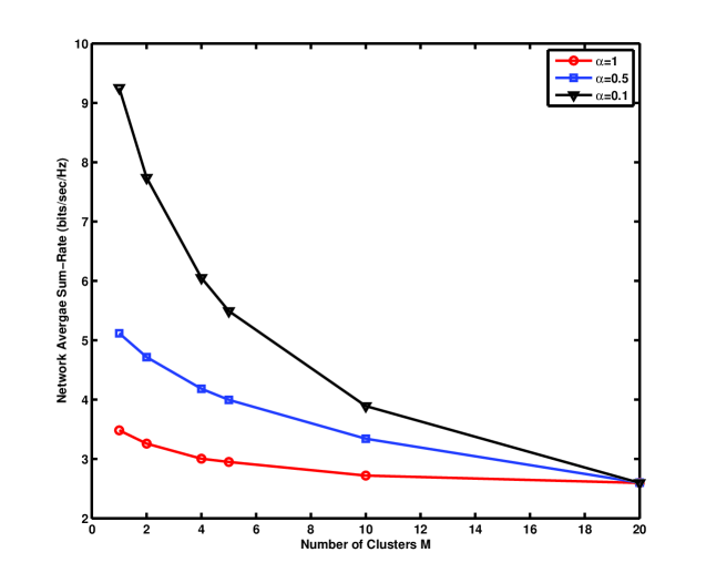
(a)

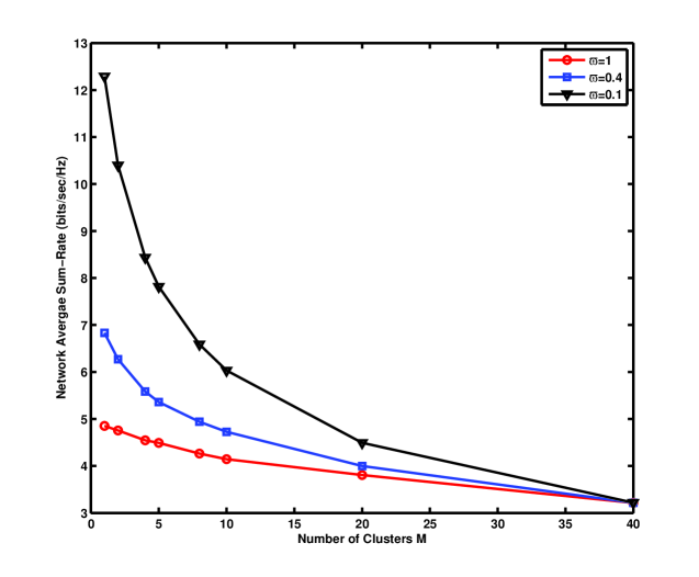
(b)

Figure 1: Network average sum-rate vs. $M$ for a) $K=20$, $\alpha=1,~{}0.5,~{}0.1$ and shadowing model with $\varpi=0.5$ and variance 1, and b) $K=40$, $\alpha=0.5$ and shadowing model with $\varpi=1,~{}0.4,~{}0.1$ and variance 1.

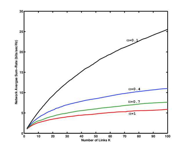
(a)

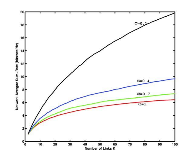
(b)

Figure 2: Network average sum-rate vs. $K$ for $M=1$ and a) shadowing model with $\varpi=0.5$ and variance 1, and $\alpha=1,~{}0.7,~{}0.4,~{}0.1$, and b) shadowing model with $\varpi=1,~{}0.7,~{}0.4,~{}0.1$ and variance 1, and $\alpha=0.5$.

IV Network Guaranteed Sum-Rate

Recalling the definition of the network guaranteed sum-rate in (7), in this section we aim to find the maximum achievable guaranteed sum-rate of the network, as well as the optimum power allocation scheme and the optimum value of $M$.

Theorem 4

The guaranteed sum-rate of the underlying network in the asymptotic case of $K\to\infty$ is obtained by

$$\bar{R}_{g}\sim\frac{W}{\hat{\alpha}}\log K,$$ (74)

which is achievable by the decentralized on-off power allocation scheme.

Proof.

In order to compute the guaranteed rate for link $l\in\mathbb{C}_{j}$, we first define the corresponding outage event as follows:

$$\mathcal{O}_{l}^{(j)} \equiv \left\{R_{l}(\textbf{{P}}^{(j)},\boldsymbol{\mathcal{L}}_{l}^{(j)})<R(h_{ll})\right\}$$ (75)

$$\equiv \left\{\log\left(1+\frac{p_{l}h_{ll}}{I_{l}+\frac{N_{0}W}{M}}\right)<R(h_{ll})\right\}.$$ (76)

In the following, we give an upper-bound and a lower-bound for $\bar{R}_{g}$ and show that these bounds converge to each other as $K\to\infty$ (or equivalently, $n\to\infty$).

Upper-bound: An upper-bound on the guaranteed sum-rate can be given by lower-bounding the outage probability as follows:

$$\mathbb{P}\left\{\mathcal{O}_{l}^{(j)}\right\} \geq \mathbb{P}\left\{\frac{p_{l}h_{ll}}{I_{l}+\frac{N_{0}W}{M}}<R(h_{ll})\right\}$$ (77)

$$= \mathbb{P}\left\{p_{l}h_{ll}-\frac{N_{0}W}{M}R(h_{ll})<I_{l}R(h_{ll})\right\},$$ (78)

in which we have used the fact that $\log(1+x)\leq x$. Denoting $\nu=h_{ll}$, we can write

$$\mathbb{P}\left\{\mathcal{O}_{l}^{(j)}\right\} \stackrel{{\scriptstyle(a)}}{{\geq}} \mathbb{P}\left\{e^{-I_{l}\xi(\nu)R(\nu)}\leq e^{\xi(\nu)\left(\frac{N_{0}W}{M}R(\nu)-p_{l}\nu\right)}\right\}$$ (79)

$$\stackrel{{\scriptstyle(b)}}{{\geq}} 1-e^{-\xi(\nu)\left(\frac{N_{0}W}{M}R(\nu)-p_{l}\nu\right)}\mathbb{E}\left[e^{-I_{l}\xi(\nu)R(\nu)}\right],$$ (80)

for some positive $\xi(\nu)$. In the above equation, $(a)$ results from (78), noting that $\xi(\nu)>0$, and $(b)$ follows from Markov’s inequality [36, p. 77], and the expectation is taken with respect to $I_{l}$. The above equation implies that finding an upper-bound for $\mathbb{E}\left[e^{-I_{l}\xi(\nu)R(\nu)}\right]$ is sufficient for the lower-bounding the outage probability. For this purpose, using (4), we can write

$$\mathbb{E}\left[e^{-I_{l}\xi(\nu)R(\nu)}\right] = \mathbb{E}\left[e^{-\xi(\nu)R(\nu)\sum_{\begin{subarray}{c}k\in\mathbb{C}_{j}\\ k\neq l\end{subarray}}\mathcal{L}_{kl}p_{k}}\right]$$ (81)

$$\stackrel{{\scriptstyle(a)}}{{=}} \prod_{\begin{subarray}{c}k\in\mathbb{C}_{j}\\ k\neq l\end{subarray}}\mathbb{E}\left[e^{-\xi(\nu)R(\nu)\mathcal{L}_{kl}p_{k}}\right]$$ (82)

$$\stackrel{{\scriptstyle(b)}}{{=}} \prod_{\begin{subarray}{c}k\in\mathbb{C}_{j}\\ k\neq l\end{subarray}}\mathbb{E}\left[e^{-\xi(\nu)R(\nu)u_{kl}\beta_{kl}h_{kl}p_{k}}\right]$$ (83)

$$\stackrel{{\scriptstyle(c)}}{{=}} \left(\mathbb{E}\left[e^{-\xi(\nu)R(\nu)u_{kl}\beta_{kl}h_{kl}p_{k}}\right]\right)^{n-1},~{}k\neq l.$$ (84)

In the above equation, $(a)$ follows from the fact that $\{\mathcal{L}_{kl}\}_{k\in\mathbb{C}_{j}}$ with $k\neq l$, and $\{p_{k}\}_{k\in\mathbb{C}_{j}}$ are mutually independent random variables, $(b)$ results from writing $\mathcal{L}_{kl}$ as $u_{kl}\beta_{kl}h_{kl}$ (from (3)), in which $u_{kl}$ is an indicator variable which takes zero when $\mathcal{L}_{kl}=0$ and one, otherwise. $(c)$ follows from the symmetry which incurs that all the terms $\mathbb{E}\left[e^{-\xi(\nu)R(\nu)u_{kl}\beta_{kl}h_{kl}p_{k}}\right]$, $k\in\mathbb{C}_{j}$, are equal. Noting that $u_{kl}$, $\beta_{kl}$, $h_{kl}$, and $p_{k}$ are independent of each other, we have

$$\mathbb{E}\left[e^{-\xi(\nu)R(\nu)u_{kl}\beta_{kl}h_{kl}p_{k}}\right] = \mathbb{E}_{\beta_{kl}}\left[\mathbb{E}_{h_{kl}}\left[\mathbb{E}_{u_{kl}}\left[\mathbb{E}_{p_{k}}\left[e^{-\xi(\nu)R(\nu)u_{kl}\beta_{kl}h_{kl}p_{k}}\right]\right]\right]\right]$$ (85)

$$\stackrel{{\scriptstyle(a)}}{{\leq}} \mathbb{E}_{\beta_{kl}}\left[\mathbb{E}_{h_{kl}}\left[\mathbb{E}_{u_{kl}}\left[(1-q_{n})+q_{n}e^{-\xi(\nu)R(\nu)u_{kl}\beta_{kl}h_{kl}}\right]\right]\right]$$ (86)

$$\stackrel{{\scriptstyle(b)}}{{=}} \mathbb{E}_{\beta_{kl}}\left[\mathbb{E}_{h_{kl}}\left[(1-q_{n})+q_{n}\left(1-\alpha+\alpha e^{-\xi(\nu)R(\nu)\beta_{kl}h_{kl}}\right)\right]\right]$$ (87)

$$\stackrel{{\scriptstyle(c)}}{{=}} \mathbb{E}_{\beta_{kl}}\left[1-\alpha q_{n}+\frac{\alpha q_{n}}{1+\beta_{kl}\xi(\nu)R(\nu)}\right]$$ (88)

$$= \mathbb{E}_{\beta_{kl}}\left[1-\frac{\alpha q_{n}\beta_{kl}\xi(\nu)R(\nu)}{1+\beta_{kl}\xi(\nu)R(\nu)}\right]$$ (89)

$$\stackrel{{\scriptstyle(d)}}{{\leq}} 1-\frac{\alpha q_{n}\varpi\xi(\nu)R(\nu)}{1+\beta_{\max}\xi(\nu)R(\nu)}$$ (90)

$$\stackrel{{\scriptstyle(e)}}{{\leq}} e^{-\frac{\hat{\alpha}q_{n}\xi(\nu)R(\nu)}{1+\beta_{\max}\xi(\nu)R(\nu)}}.$$ (91)

In the above equation, $(a)$ follows from the fact that $e^{-\theta x}\leq(1-x)+xe^{-\theta}$, $\forall\theta\geq 0$ and $0\leq x\leq 1$, noting that $\mathbb{E}[p_{k}]=q_{n}$. $(b)$ results from the definition of $u_{kl}$, which is an indicator variable taking zero with probability $1-\alpha$ and one, with probability $\alpha$. $(c)$ follows from the fact that as $h_{kl}$ is exponentially-distributed, we have $\mathbb{E}_{h_{kl}}\left[e^{-\xi(\nu)R(\nu)\beta_{kl}h_{kl}}\right]=\frac{1}{1+\beta_{kl}\xi(\nu)R(\nu)}$. $(d)$ results from the facts that $\beta_{kl}\leq\beta_{\max}$ and $\mathbb{E}[\beta_{kl}]=\varpi$. Finally, $(e)$ follows from the fact that $1-x\leq e^{-x}$, $\forall x$ and noting that $\alpha\varpi=\hat{\alpha}$.

Combining (84) and (91) and substituting into (80) yields

$$\mathbb{P}\left\{\mathcal{O}_{l}^{(j)}\right\} \geq 1-e^{-\xi(\nu)\left(\frac{N_{0}W}{M}R(\nu)-p_{l}\nu\right)}e^{-\frac{(n-1)\hat{\alpha}q_{n}\xi(\nu)R(\nu)}{1+\beta_{\max}\xi(\nu)R(\nu)}}$$ (92)

$$= 1-e^{-\xi(\nu)R(\nu)\left(\frac{(n-1)\hat{\alpha}q_{n}}{1+\beta_{\max}\xi(\nu)R(\nu)}+\frac{N_{0}W}{M}\right)\left(1-\frac{t(\nu)}{R(\nu)}\right)},$$ (93)

where $t(\nu)\triangleq\frac{p_{l}\nu}{\frac{(n-1)\hat{\alpha}q_{n}}{1+\beta_{\max}\xi(\nu)R(\nu)}+\frac{N_{0}W}{M}}$.

Consider the cases of $\mathbb{E}\{I_{l}\}=\omega(1)$ (strong interference) or $\mathbb{E}\{I_{l}\}=\Theta(1)$ (moderate interference). Let us define $\gamma\triangleq\min\left(1,\frac{M(n-1)q_{n}\hat{\alpha}}{N_{0}W}\right)$. Setting $\xi(\nu)\triangleq\frac{\frac{\gamma}{2}\frac{N_{0}W}{M}}{\beta_{\max}R(\nu)\left((n-1)\hat{\alpha}q_{n}-\frac{\gamma}{2}\frac{N_{0}W}{M}\right)}$, we have $\frac{(n-1)\hat{\alpha}q_{n}}{1+\beta_{\max}\xi(\nu)R(\nu)}+\frac{N_{0}W}{M}=(n-1)\hat{\alpha}q_{n}+(1-\frac{\gamma}{2})\frac{N_{0}W}{M}$, and as a result,

$$\mathbb{P}\left\{\mathcal{O}_{l}^{(j)}\right\} \geq 1-e^{-\frac{\frac{\gamma}{2}\frac{N_{0}W}{M}\left[(n-1)\hat{\alpha}q_{n}+(1-\frac{\gamma}{2})\frac{N_{0}W}{M}\right]}{\beta_{\max}\left[(n-1)\hat{\alpha}q_{n}-\frac{\gamma}{2}\frac{N_{0}W}{M}\right]}\left(1-\frac{t(\nu)}{R(\nu)}\right)}$$ (94)

$$\geq 1-e^{-\frac{\gamma N_{0}W}{2M\beta_{\max}}\left(1-\frac{t(\nu)}{R(\nu)}\right)}.$$ (95)

Since $\frac{\gamma N_{0}W}{2M\beta_{\max}}=\Theta(1)$, it follows that the necessary condition to have $\mathbb{P}\left\{\mathcal{O}_{l}^{(j)}\right\}\to 0$ is having $R(\nu)\lesssim t(\nu)=\frac{p_{l}\nu}{(n-1)\hat{\alpha}q_{n}+(1-\frac{\gamma}{2})\frac{N_{0}W}{M}}$. In other words,

$$R^{*}(\nu)\lesssim\frac{p_{l}\nu}{(n-1)\hat{\alpha}q_{n}+(1-\frac{\gamma}{2})\frac{N_{0}W}{M}},$$ (96)

which implies that $\bar{R}_{g}$ defined in (7) is upper bounded by

$$\bar{R}_{g} \lesssim nW\mathbb{E}_{\nu}\left[\frac{p_{l}\nu}{(n-1)\hat{\alpha}q_{n}+(1-\frac{\gamma}{2})\frac{N_{0}W}{M}}\right]$$ (97)

$$= \frac{nW\mathbb{E}_{\nu}\left[p_{l}\nu\right]}{(n-1)\hat{\alpha}q_{n}+(1-\frac{\gamma}{2})\frac{N_{0}W}{M}}.$$ (98)

Now, defining $\Psi_{n}\triangleq\log n+2\log\log n$, we have

$$\mathbb{E}_{\nu}\left[p_{l}\nu\right] \leq \mathbb{E}\left[p_{l}\nu|\nu\leq\Psi_{n}\right]\mathbb{P}\{\nu\leq\Psi_{n}\}+\mathbb{E}\left[p_{l}\nu|\nu>\Psi_{n}\right]\mathbb{P}\{\nu>\Psi_{n}\}$$ (99)

$$\stackrel{{\scriptstyle(a)}}{{\leq}} q_{n}\Psi_{n}+\mathbb{E}\left[\nu|\nu>\Psi_{n}\right]\mathbb{P}\{\nu>\Psi_{n}\}$$ (100)

$$\stackrel{{\scriptstyle(b)}}{{=}} q_{n}\Psi_{n}+(\Psi_{n}+1)e^{-\Psi_{n}}$$ (101)

$$\stackrel{{\scriptstyle(c)}}{{\sim}} q_{n}\log n.$$ (102)

In the above equation, $(a)$ comes from the facts that

$$\mathbb{E}\left[p_{l}\nu|\nu\leq\Psi_{n}\right]\mathbb{P}\{\nu\leq\Psi_{n}\}\leq\Psi_{n}\mathbb{E}\left[p_{l}|\nu\leq\Psi_{n}\right]\mathbb{P}\{\nu\leq\Psi_{n}\}\leq\Psi_{n}\mathbb{E}[p_{l}]=\Psi_{n}q_{n},$$

and $0\leq p_{l}\leq 1$. $(b)$ results from the fact that $\nu$ is exponentially-distributed. $(c)$ follows from the facts that i) as we are considering the strong and moderate interference scenarios, it yields that $(n-1)\hat{\alpha}q_{n}=\Omega(1)$, or equivalently, $q_{n}=\Omega(\frac{1}{n})$, and ii) the term $(\Psi_{n}+1)e^{-\Psi_{n}}$ scales as $\frac{1}{n\log n}$ (due to the definition of $\Psi_{n}$) which is negligible with respect to the first term $q_{n}\Psi_{n}$. Combining (98) and (102) yields

$$\bar{R}_{g} \lesssim \frac{Wnq_{n}\log n}{(n-1)\hat{\alpha}q_{n}+(1-\frac{\gamma}{2})\frac{N_{0}W}{M}}$$ (103)

$$\lesssim \frac{W}{\hat{\alpha}}\log n$$ (104)

$$\lesssim \frac{W}{\hat{\alpha}}\log K.$$ (105)

In the case of weak interference, we have

$$\bar{R}_{g} \leq nW\frac{\mathbb{E}[p_{l}\nu]}{\frac{N_{0}W}{M}}$$ (106)

$$= \frac{Mn}{N_{0}}\mathbb{E}[p_{l}\nu].$$ (107)

Rewriting (101), we obtain

$$\mathbb{E}[p_{l}\nu] \leq q_{n}\Psi_{n}+(\Psi_{n}+1)e^{-\Psi_{n}},\quad\forall\Psi_{n}>0.$$ (108)

Selecting $\Psi_{n}=\log(q_{n}^{-2})$ and defining $\varepsilon\triangleq nq_{n}$, we have

$$\bar{R}_{g} \lesssim \frac{2M\varepsilon}{N_{0}}\left(\log n-\log(\varepsilon^{-1})\right).$$ (109)

As in the weak interference scenario we have $\varepsilon=o(1)$, it follows from the above equation that $\bar{R}_{g}=o(W\log n)$ in this scenario. Comparing with (105), it follows that

$$\bar{R}_{g}\lesssim\frac{W}{\hat{\alpha}}\log K.$$ (110)

Lower-bound For the lower-bound, we consider the on-off power allocation scheme with $\tau_{n}=\log n-2\log\log n$. Also, assume that $M=1$ (or equivalently, $n=K$). Noting $q_{n}=e^{-\tau_{n}}$, we obtain

$$\mathbb{E}[I_{l}]=(n-1)\hat{\alpha}q_{n}=\Theta(\log^{2}n).$$ (111)

Therefore, using the result of Lemma 1, it is realized that with probability one $(n-1)\hat{\alpha}q_{n}(1-\epsilon)\leq I_{l}\leq(n-1)\hat{\alpha}q_{n}(1+\epsilon)$, for some $\epsilon=o(1)$. In other words, defining

$$\varPhi(\nu)\triangleq\log\left(1+\frac{p_{l}\nu}{(n-1)\hat{\alpha}q_{n}(1+\epsilon)+\frac{N_{0}W}{M}}\right),$$ (112)

it follows that

$$\mathbb{P}\left\{R_{l}(\textbf{{P}}^{(j)},\boldsymbol{\mathcal{L}}_{l}^{(j)})<\varPhi(\nu)\right\}=o(1),$$ (113)

which implies that $R^{*}(\nu)\geq\varPhi(\nu)$. As a result,

$$\bar{R}_{g} \geq nW\mathbb{E}[\varPhi(\nu)]$$ (114)

$$= nW\mathbb{E}\left[\log\left(1+\frac{p_{l}\nu}{(n-1)\hat{\alpha}q_{n}(1+\epsilon)+\frac{N_{0}W}{M}}\right)\right]$$ (115)

$$\stackrel{{\scriptstyle(a)}}{{=}} nW\int_{\tau_{n}}^{\infty}\log\left(1+\frac{\nu}{(n-1)\hat{\alpha}q_{n}(1+\epsilon)+\frac{N_{0}W}{M}}\right)e^{-\nu}d\nu$$ (116)

$$\geq nW\int_{\tau_{n}}^{\Psi_{n}}\log\left(1+\frac{\nu}{(n-1)\hat{\alpha}q_{n}(1+\epsilon)+\frac{N_{0}W}{M}}\right)e^{-\nu}d\nu,$$ (117)

where $\Psi_{n}\triangleq\log n+2\log\log n$ and $(a)$ follows from the on-off power allocation assumption. As $(n-1)\hat{\alpha}q_{n}(1+\epsilon)=\Theta(\log^{2}n)$, it follows that $\frac{\nu}{(n-1)\hat{\alpha}q_{n}(1+\epsilon)+\frac{N_{0}W}{M}}=o(1)$ in the interval $[\tau_{n},\Psi_{n}]$, which implies that

$$\log\left(1+\frac{\nu}{(n-1)\hat{\alpha}q_{n}(1+\epsilon)+\frac{N_{0}W}{M}}\right)\sim\frac{\nu}{(n-1)\hat{\alpha}q_{n}(1+\epsilon)+\frac{N_{0}W}{M}},$$ (118)

in the interval of integration $[\tau_{n},\Psi_{n}]$. Hence,

$$\bar{R}_{g} \gtrsim nW\int_{\tau_{n}}^{\Psi_{n}}\frac{\nu}{(n-1)\hat{\alpha}q_{n}(1+\epsilon)+\frac{N_{0}W}{M}}e^{-\nu}d\nu$$ (119)

$$= \frac{nW}{(n-1)\hat{\alpha}q_{n}(1+\epsilon)+\frac{N_{0}W}{M}}\int_{\tau_{n}}^{\Psi_{n}}\nu e^{\nu}d\nu$$ (120)

$$= \frac{nW}{(n-1)\hat{\alpha}q_{n}(1+\epsilon)+\frac{N_{0}W}{M}}\left((\tau_{n}+1)e^{-\tau_{n}}-(\Psi_{n}+1)e^{-\Psi_{n}}\right)$$ (121)

$$\stackrel{{\scriptstyle(a)}}{{\sim}} \frac{nW\tau_{n}q_{n}}{(n-1)\hat{\alpha}q_{n}(1+\epsilon)+\frac{N_{0}W}{M}}$$ (122)

$$\sim \frac{W}{\hat{\alpha}}\log n$$ (123)

$$= \frac{W}{\hat{\alpha}}\log K,$$ (124)

where $(a)$ results from the facts that $(\Psi_{n}+1)e^{-\Psi_{n}}\ll(\tau_{n}+1)e^{-\tau_{n}}$ and $e^{-\tau_{n}}=q_{n}$. Combining the above equation with (110), the proof of Theorem 4 follows. ∎

Remark 7- Similar to the proof steps of Theorem 1, it can be shown that the optimum value of $M$ is equal to one. In fact, since the maximum guaranteed sum-rate of the network is achieved in the strong interference scenario in which the interference term scales as $n\hat{\alpha}q_{n}$ with probability one, it follows that the maximum network average sum-rate and the network guaranteed sum-rate are equal. Therefore, the optimum spectrum sharing for maximizing the network guaranteed sum-rate is the same as the one maximizing the average sum-rate of the network ($M=1$).

V Conclusion

In this paper, a distributed single-hop wireless network with $K$ links was considered, where the links were partitioned into a fixed number ($M$) of clusters each operating in a subchannel with bandwidth $\frac{W}{M}$. The subchannels were assumed to be orthogonal to each other. A general shadow-fading model, described by parameters $(\alpha,\varpi)$, was considered where $\alpha$ denotes the probability of shadowing and $\varpi$ ($\varpi\leq 1$) represents the average cross-link gains. The maximum achievable network throughput was studied in the asymptotic regime of $K\to\infty$. In the first part of the paper, the network throughput is defined as the average sum-rate of the network, which is shown to scale as $\Theta(\log K)$. Moreover, it was proved that in the strong interference scenario, the optimum power allocation strategy for each user was a threshold-based on-off scheme. In the second part, the network throughput is defined as the guaranteed sum-rate, when the outage probability approaches zero. In this scenario, it was demonstrated that the on-off power allocation scheme maximizes the network guaranteed sum-rate, which scales as $\frac{W}{\hat{\alpha}}\log K$. Moreover, the optimum spectrum sharing for maximizing the average sum-rate and guaranteed sum-rate is achieved at $M=1$.

Appendix A Proof of Lemma 1

Let us define $\chi_{k}\triangleq\mathcal{L}_{ki}p_{k}$, where $\mathcal{L}_{ki}$ is independent of $p_{k}$, for $k\neq i$. Under a quasi-static Rayleigh fading channel model, it is concluded that $\chi_{k}$’s are independent and identically distributed (i.i.d.) random variables with

$$\mathbb{E}\left[\chi_{k}\right] = \mathbb{E}\left[\mathcal{L}_{ki}p_{k}\right]=\hat{\alpha}q_{n},$$ (A-1)

$$\textrm{Var}\left[\chi_{k}\right] = \mathbb{E}\left[\chi^{2}_{k}\right]-\mathbb{E}^{2}\left[\chi_{k}\right]$$ (A-2)

$$\stackrel{{\scriptstyle(a)}}{{\leq}} 2\alpha\kappa q_{n}-(\hat{\alpha}q_{n})^{2},$$ (A-3)

where $\mathbb{E}\left[h_{ki}^{2}\right]=2$ and $\hat{\alpha}\triangleq\alpha\varpi$. Also, $(a)$ follows from the fact that $p_{k}^{2}\leq p_{k}$. Thus, $\mathbb{E}[p_{k}^{2}]\leq\mathbb{E}[p_{k}]=q_{n}$. The interference $I_{i}=\sum_{\begin{subarray}{c}k\in\mathbb{C}_{j}\\ k\neq i\end{subarray}}\chi_{k}$ is a random variable with mean $\mu_{n}$ and variance $\vartheta_{n}^{2}$, where

$$\mu_{n} \triangleq \mathbb{E}\left[I_{i}\right]=(n-1)\hat{\alpha}q_{n},$$ (A-4)

$$\vartheta_{n}^{2} \triangleq \textrm{Var}\left[I_{i}\right]\leq(n-1)(2\alpha\kappa q_{n}-(\hat{\alpha}q_{n})^{2})\leq(n-1)(2\alpha\kappa q_{n}).$$ (A-5)

Using the Central Limit Theorem [37, p. 183], we obtain

$$\mathbb{P}\{|I_{i}-\mu_{n}|<\psi_{n}\} \approx 1-Q\left(\dfrac{\psi_{n}}{\vartheta_{n}}\right)$$ (A-6)

$$\stackrel{{\scriptstyle(a)}}{{\geq}} 1-e^{-\frac{\psi^{2}_{n}}{2\vartheta^{2}_{n}}},$$ (A-7)

for all $\psi_{n}>0$ such that $\psi_{n}=o\left(n^{\frac{1}{6}}\vartheta_{n}\right)$. In the above equation, the $Q(.)$ function is defined as $Q(x)\triangleq\frac{1}{\sqrt{2\pi}}\int_{x}^{\infty}e^{-u^{2}/2}du$, and $(a)$ follows from the fact that $Q(x)\leq e^{-\frac{x^{2}}{2}}$, $\forall x>0$. Selecting $\psi_{n}=\left(nq_{n}\right)^{\frac{1}{8}}\sqrt{2}\vartheta_{n}$, we obtain

$$\mathbb{P}\{|I_{i}-\mu_{n}|<\psi_{n}\} \geq 1-e^{-\left(nq_{n}\right)^{\frac{1}{4}}}.$$ (A-8)

Therefore, defining $\varepsilon\triangleq\frac{\psi_{n}}{\mu_{n}}=O\left((nq_{n})^{-\frac{3}{8}}\right)$, we have

$$\mathbb{P}\{\mu_{n}\left(1-\varepsilon\right)\leq I_{i}\leq\mu_{n}\left(1+\varepsilon\right)\} \geq 1-e^{-\left(nq_{n}\right)^{\frac{1}{4}}}.$$ (A-9)

Noting that $nq_{n}\to\infty$, it follows that $I_{i}\sim\mu_{n}$, with probability one. Now, we show a stronger statement, which is, the contribution of the realizations in which $|I_{i}-\mu_{n}|>\psi_{n}$ in the network average sum-rate is negligible. For this purpose, we give a lower-bound and an upper-bound for the network average sum-rate and show that these bounds converge to each other in the strong interference regime, when $nq_{n}\to\infty$. A lower-bound denoted by $\bar{R}_{ave}^{(L)}$, can be given by

$$\bar{R}_{ave}^{(L)} \triangleq nW\mathbb{E}\left.\left[\log\left(1+\frac{\hat{p}_{i}h_{ii}}{I_{i}+\frac{N_{0}W}{M}}\right)\right||I_{i}-\mu_{n}|<\psi_{n}\right]\mathbb{P}\{|I_{i}-\mu_{n}|<\psi_{n}\}$$ (A-10)

$$\geq nW\mathbb{E}\left[\log\left(1+\frac{\hat{p}_{i}h_{ii}}{\mu_{n}(1+\varepsilon)+\frac{N_{0}W}{M}}\right)\right]\left[1-e^{-\left(nq_{n}\right)^{\frac{1}{4}}}\right],$$ (A-11)

which scales as $\frac{W}{\hat{\alpha}}\log n$ (as shown in the proof of Theorem 1, by optimizing the power allocation function). An upper-bound for the network average sum-rate, denoted by $\bar{R}_{ave}^{(U)}$, can be given as

$$\bar{R}_{ave}^{(U)} = nW\mathbb{E}\left.\left[\log\left(1+\frac{\hat{p}_{i}h_{ii}}{I_{i}+\frac{N_{0}W}{M}}\right)\right||I_{i}-\mu_{n}|<\psi_{n}\right]\mathbb{P}\{|I_{i}-\mu_{n}|<\psi_{n}\}+$$ (A-12)

$$nW\mathbb{E}\left.\left[\log\left(1+\frac{\hat{p}_{i}h_{ii}}{I_{i}+\frac{N_{0}W}{M}}\right)\right||I_{i}-\mu_{n}|\geq\psi_{n}\right]\mathbb{P}\{|I_{i}-\mu_{n}|\geq\psi_{n}\}$$

$$\leq \bar{R}_{ave}^{(L)}+nW\mathbb{E}\left[\log\left(1+\frac{\hat{p}_{i}h_{ii}}{\frac{N_{0}W}{M}}\right)\right]e^{-\left(nq_{n}\right)^{\frac{1}{4}}}$$ (A-13)

$$\stackrel{{\scriptstyle(a)}}{{\leq}} \bar{R}_{ave}^{(L)}+nW\mathbb{E}\left[\dfrac{\hat{p}_{i}h_{ii}}{\frac{N_{0}W}{M}}\right]e^{-\left(nq_{n}\right)^{\frac{1}{4}}}$$ (A-14)

$$\stackrel{{\scriptstyle(b)}}{{=}} \bar{R}_{ave}^{(L)}+WO(nq_{n}\log n)e^{-\left(nq_{n}\right)^{\frac{1}{4}}}$$ (A-15)

$$\stackrel{{\scriptstyle(c)}}{{\sim}} \bar{R}_{ave}^{(L)}.$$ (A-16)

In the above equation, $(a)$ follows from the fact that $\log(1+x)\leq x$, $(b)$ comes from the facts that $\mathbb{E}\{p_{i}h_{ii}\}\lesssim q_{n}\log n$ (this is shown in the proof of Theorem 4) and $\frac{N_{0}W}{M}$ is fixed, and finally, $(c)$ results from the fact that as $nq_{n}\to\infty$, $nq_{n}e^{-(nq_{n})^{\frac{1}{4}}}\to 0$. The above equation implies that substituting $I_{i}$ by its mean ($(n-1)\hat{\alpha}q_{n}$) does not affect the analysis of the network average sum-rate in the asymptotic case of $K\to\infty$.

Appendix B Proof of Lemma 2

Denoting $\mathbb{T}_{j}\triangleq\{l\in\mathbb{C}_{j}~{}|~{}h_{ll}>h_{Th}\}$, the cardinality of the set $\mathbb{T}_{j}$ is a binomial random variable with the mean $n\mathbb{P}\{h_{ll}>h_{Th}\}$. From (6), we have

$$\bar{R}_{ave}=\sum_{j=1}^{M}\mathbb{E}\left[\sum_{l\in\mathbb{C}_{j}}R_{l}(\hat{\textbf{{P}}}^{(j)},\boldsymbol{\mathcal{L}}_{l}^{(j)})\right],$$ (B-1)

where

$$\mathbb{E}\left[\sum_{l\in\mathbb{C}_{j}}R_{l}(\hat{\textbf{{P}}}^{(j)},\boldsymbol{\mathcal{L}}_{l}^{(j)})\right]=\mathbb{E}\left[\sum_{l\in\mathbb{T}_{j}}R_{l}(\hat{\textbf{{P}}}^{(j)},\boldsymbol{\mathcal{L}}_{l}^{(j)})\right]+\mathbb{E}\left[\sum_{l\in\mathbb{T}^{C}_{j}}R_{l}(\hat{\textbf{{P}}}^{(j)},\boldsymbol{\mathcal{L}}_{l}^{(j)})\right],$$ (B-2)

in which $\mathbb{T}_{j}^{C}$ denotes the complement of $\mathbb{T}_{j}$. Note that

$$\mathbb{E}\left[\sum_{l\in\mathbb{T}_{j}}R_{l}(\hat{\textbf{{P}}}^{(j)},\boldsymbol{\mathcal{L}}_{l}^{(j)})\right] = n\frac{W}{M}\mathbb{E}\left.\left[\log\left(1+\dfrac{h_{ll}\hat{p}_{l}}{I_{l}+\frac{N_{0}W}{M}}\right)\right|h_{ll}>h_{Th}\right]\mathbb{P}\{h_{ll}>h_{Th}\}$$ (B-3)

$$\leq n\frac{W}{M}\mathbb{E}\left.\left[\log\left(1+\dfrac{h_{ll}}{\frac{N_{0}W}{M}}\right)\right|h_{ll}>h_{Th}\right]\mathbb{P}\{h_{ll}>h_{Th}\}$$ (B-4)

$$\stackrel{{\scriptstyle(a)}}{{\leq}} \dfrac{n}{N_{0}}e^{-h_{Th}}\mathbb{E}\left[h_{ll}|h_{ll}>h_{Th}\right]$$ (B-5)

$$= \dfrac{n}{N_{0}}e^{-h_{Th}}(1+h_{Th}),$$ (B-6)

where $(a)$ follows from $\log(1+x)\leq x$, for $x>0$. It is observed that for $h_{Th}=c\log n$, where $c>1$, the right hand side of (B-6) tends to zero as $n\rightarrow\infty$. Thus,

$$\lim_{n\rightarrow\infty}\mathbb{E}\left[\sum_{l\in\mathbb{T}_{j}}R_{l}(\hat{\textbf{{P}}}^{(j)},\boldsymbol{\mathcal{L}}_{l}^{(j)})\right]=0.$$ (B-7)

Consequently,

$$\lim_{n\rightarrow\infty}\sum_{j=1}^{M}\mathbb{E}\left[\sum_{l\in\mathbb{T}_{j}}R_{l}(\hat{\textbf{{P}}}^{(j)},\boldsymbol{\mathcal{L}}_{l}^{(j)})\right]=0,$$ (B-8)

and this completes the proof of the lemma.

Appendix C Proof of Lemma 3

Using (34), we have

$$\mathbb{E}[\Xi_{i}(\hat{p}_{i},h_{ii})] \approx \dfrac{W}{M\lambda}\mathbb{E}[h_{ii}\hat{p}_{i}]+n\dfrac{\alpha W\mu}{M\lambda^{\prime}}\left(1-\dfrac{\varpi}{\lambda^{\prime}}\mathbb{E}[\hat{p}_{i}]+\dfrac{2\kappa}{\lambda^{\prime 2}}\mathbb{E}[\hat{p}_{i}^{2}]-\dfrac{6\eta}{\lambda^{\prime 3}}\mathbb{E}[\hat{p}_{i}^{3}]\right)+$$ (C-2)

$$n(1-\alpha)\dfrac{W\mu}{M\lambda^{\prime}}$$

$$\stackrel{{\scriptstyle(a)}}{{=}} \dfrac{W}{M\lambda}(1+\tau_{n})q_{n}-\dfrac{n\hat{\alpha}W}{M\lambda^{\prime 2}}(1+\tau_{n})q_{n}^{2}+\dfrac{n\alpha W2\kappa}{M\lambda^{\prime 3}}(1+\tau_{n})q_{n}^{2}-$$

$$\dfrac{n\alpha W6\eta}{M\lambda^{\prime 4}}(1+\tau_{n})q_{n}^{2}+\dfrac{nW}{M\lambda^{\prime}}(1+\tau_{n})q_{n}$$

$$\stackrel{{\scriptstyle(b)}}{{\approx}} \dfrac{W}{M\hat{\alpha}}\left(1+\tau_{n}+\dfrac{\xi_{1}}{n^{2}}(1+\tau_{n})e^{\tau_{n}}-\dfrac{\xi_{2}}{n^{3}}(1+\tau_{n})e^{2\tau_{n}}\right),$$ (C-3)

where $\xi_{1}\triangleq\dfrac{2\kappa}{\varpi\hat{\alpha}}$ and $\xi_{2}\triangleq\dfrac{6\eta}{\varpi\hat{\alpha}^{2}}$. In the above equation, $(a)$ follows from the fact that $\mathbb{E}[h_{ii}\hat{p}_{i}]=\mu=(1+\tau_{n})q_{n}$, and $(b)$ results from i) $\lambda=(n-1)\hat{\alpha}q_{n}+\frac{N_{0}W}{M}\approx n\hat{\alpha}q_{n}$ and $\lambda^{\prime}\approx n\hat{\alpha}q_{n}$ incurred by the fact that $\lambda\gg 1$, and ii) $q_{n}=e^{-\tau_{n}}$. Since $n\hat{\alpha}q_{n}\to\infty$, it follows that the right hand side of (C-3) is a monotonically increasing function of $\tau_{n}$, which attains its maximum when $\tau_{n}$ takes its maximum feasible value. The maximum feasible value of $\tau_{n}$, denoted as $\hat{\tau}_{n}$, can be obtained as

$$n\hat{\alpha}e^{-\tau_{n}}\to\infty\Longrightarrow\hat{\tau}_{n}\sim\log n.$$ (C-4)

Thus, the maximum achievable value for $\mathbb{E}[\Xi_{i}(\hat{p}_{i},h_{ii})]$ scales as $\dfrac{W}{M\hat{\alpha}}\log n$.

Appendix D Proof of Lemma 4

$i)$ Using (10) and assuming that all users follow the on-off power allocation policy, $\mathbb{E}[u_{i}(\hat{p}_{i},h_{ii})]$ can be expressed as

$$\mathbb{E}[u_{i}(\hat{p}_{i},h_{ii})]=\sum_{l\in\mathbb{C}_{j}}\mathbb{E}\left[R_{l}(\hat{\textbf{{P}}}^{(j)},\boldsymbol{\mathcal{L}}_{l}^{(j)})\right],~{}~{}j=1,...,M,$$ (D-1)

where the expectation is computed with respect to $h_{ll}$ and $I_{l}$. Noting that $q_{n}=\mathbb{P}\left\{h_{ll}>\tau_{n}\right\}$, we have

$$\mathbb{E}\left[R_{l}(\hat{\textbf{{P}}}^{(j)},\boldsymbol{\mathcal{L}}_{l}^{(j)})\right] = \mathbb{E}\left.\left[R_{l}(\hat{\textbf{{P}}}^{(j)},\boldsymbol{\mathcal{L}}_{l}^{(j)})\right|h_{ll}>\tau_{n}\right]\mathbb{P}\left\{h_{ll}>\tau_{n}\right\}+$$

$$\mathbb{E}\left.\left[R_{l}(\hat{\textbf{{P}}}^{(j)},\boldsymbol{\mathcal{L}}_{l}^{(j)})\right|h_{ll}\leq\tau_{n}\right]\mathbb{P}\left\{h_{ll}\leq\tau_{n}\right\}$$

$$= q_{n}\mathbb{E}\left.\left[R_{l}(\hat{\textbf{{P}}}^{(j)},\boldsymbol{\mathcal{L}}_{l}^{(j)})\right|h_{ll}>\tau_{n}\right]+(1-q_{n})\mathbb{E}\left.\left[R_{l}(\hat{\textbf{{P}}}^{(j)},\boldsymbol{\mathcal{L}}_{l}^{(j)})\right|h_{ll}\leq\tau_{n}\right].$$

Since for $h_{ll}\leq\tau_{n}$, $\hat{p}_{l}=0$, it is concluded that

$$\mathbb{E}\left[R_{l}(\hat{\textbf{{P}}}^{(j)},\boldsymbol{\mathcal{L}}_{l}^{(j)})\right]=\dfrac{q_{n}W}{M}\mathbb{E}\left.\left[\log\left(1+\dfrac{h_{ll}}{I_{l}+\frac{N_{0}W}{M}}\right)\right|h_{ll}>\tau_{n}\right].$$ (D-3)

For large values of $K$, we can apply Lemma 1 to obtain

$$\mathbb{E}\left[R_{l}(\hat{\textbf{{P}}}^{(j)},\boldsymbol{\mathcal{L}}_{l}^{(j)})\right] \approx \dfrac{q_{n}W}{M}\mathbb{E}\left.\left[\log\left(1+\dfrac{h_{ll}}{(n-1)\hat{\alpha}q_{n}+\frac{N_{0}W}{M}}\right)\right|h_{ll}>\tau_{n}\right]$$ (D-4)

$$= \dfrac{q_{n}W}{M}\mathbb{E}\left.\left[\log\left(1+\dfrac{h_{ll}}{\lambda}\right)\right|h_{ll}>\tau_{n}\right],$$ (D-5)

where the expectation is computed with respect to $h_{ll}$. Using the Taylor series for $\log(1+x)$, (D-5) can be written as

$$\mathbb{E}\left[R_{l}(\hat{\textbf{{P}}}^{(j)},\boldsymbol{\mathcal{L}}_{l}^{(j)})\right] \approx \dfrac{q_{n}W}{M}\sum_{k=1}^{\infty}\dfrac{(-1)^{k-1}}{k\lambda^{k}}\mathbb{E}\left.\left[h_{ll}^{k}\right|h_{ll}>\tau_{n}\right]$$ (D-6)

$$\stackrel{{\scriptstyle(a)}}{{\approx}} \dfrac{q_{n}W}{M}\sum_{k=1}^{\infty}\dfrac{(-1)^{k-1}}{k(n\hat{\alpha}q_{n})^{k}}\mathbb{E}\left.\left[h_{ll}^{k}\right|h_{ll}>\tau_{n}\right]$$ (D-7)

$$\stackrel{{\scriptstyle(b)}}{{\approx}} \dfrac{q_{n}W}{M}\sum_{k=1}^{\infty}\dfrac{(-1)^{k-1}\tau_{n}^{k}}{k(n\hat{\alpha}q_{n})^{k}}$$ (D-8)

$$= \dfrac{q_{n}W}{M}\log\left(1+\frac{\tau_{n}}{n\hat{\alpha}q_{n}}\right)$$ (D-9)

$$\stackrel{{\scriptstyle(c)}}{{=}} \dfrac{e^{-\tau_{n}}W}{M}\log\left(1+\frac{\tau_{n}e^{\tau_{n}}}{n\hat{\alpha}}\right),$$ (D-10)

where $(a)$ follows from the fact that for large values of $n$, $\lambda\approx n\hat{\alpha}q_{n}$. Also, $(b)$ results from the fact that under a Rayleigh fading channel model,

$$\mathbb{E}\left.\left[h_{ll}\right|h_{ll}>\tau_{n}\right]=1+\tau_{n},$$ (D-11)

$$\mathbb{E}\left.\left[h_{ll}^{k}\right|h_{ll}>\tau_{n}\right]=\tau_{n}^{k}+k\mathbb{E}\left.\left[h_{ll}^{k-1}\right|h_{ll}>\tau_{n}\right].$$ (D-12)

Since $\lambda\gg 1$, the term $\frac{\mathbb{E}\left.\left[h_{ll}^{k-1}\right|h_{ll}>\tau_{n}\right]}{\lambda^{k}}\ll\frac{\mathbb{E}\left.\left[h_{ll}^{k-1}\right|h_{ll}>\tau_{n}\right]}{\lambda^{k-1}}$, which implies that we can neglect this term and simply write $\mathbb{E}\left.\left[h_{ll}^{k}\right|h_{ll}>\tau_{n}\right]\approx\tau_{n}^{k}$. $(c)$ results from $q_{n}=e^{-\tau_{n}}$. Thus, (D-1) can be simplified as

$$\mathbb{E}[u_{i}(\hat{p}_{i},h_{ii})]\approx\dfrac{ne^{-\tau_{n}}W}{M}\log\left(1+\frac{\tau_{n}e^{\tau_{n}}}{n\hat{\alpha}}\right).$$ (D-13)

In order to find the optimum threshold value:

$$\hat{\tau}_{n}=\arg~{}\max_{\tau_{n}}~{}\mathbb{E}[u_{i}(\hat{p}_{i},h_{ii})],$$ (D-14)

we set the derivative of the right hand side of (D-13) with respect to $\tau_{n}$ to zero:

$$-e^{-\hat{\tau_{n}}}\log\left(1+\frac{\hat{\tau}_{n}e^{\hat{\tau}_{n}}}{n\hat{\alpha}}\right)+\frac{1+\hat{\tau}_{n}}{n\hat{\alpha}+\hat{\tau}_{n}e^{\hat{\tau}_{n}}}=0,$$ (D-15)

which after some manipulations yields

$$\hat{\tau}_{n}=\log n-2\log\log n+O(1).$$ (D-16)

$ii)$ Using (D-16), it is concluded that

$$q_{n} = e^{-\tau_{n}}$$ (D-17)

$$= \delta\dfrac{\log^{2}n}{n},$$ (D-18)

where $\delta$ is a constant.

$iii)$ Using (D-16), we have

$$\frac{\hat{\tau}_{n}e^{\hat{\tau}_{n}}}{n\hat{\alpha}}=\Theta\left(\frac{1}{\log n}\right),$$ (D-19)

which implies that the right hand side of (D-13) can be written as

R​H (D-13) $$\approx \frac{W\hat{\tau}_{n}}{M\hat{\alpha}}.$$ (D-20)

Thus, the maximum value for $\mathbb{E}[u_{i}(\hat{p}_{i},h_{ii})]$ in (D-13) scales as $\dfrac{W}{M\hat{\alpha}}\log n$.

Appendix E Proof of Theorem 3

Let us define $\mathbb{A}_{j}$ as the set of active links in cluster $j$. The random variable $m_{j}$ denotes the cardinality of the set $\mathbb{A}_{j}$. Noting that for $M=\Theta(K)$, $\lim_{K\to\infty}\frac{M}{K}$ is constant, it is concluded that $n$ and $m_{j}\in[1,n]$ do not grow with $K$. To obtain the network average sum-rate, we assume that among $M$ clusters, $\Gamma$ clusters have $m_{j}=1$ and the rest have $m_{j}>1$. We first obtain an upper bound on the average sum-rate in each cluster when $m_{j}=1$, $1\leq j\leq M$. Clearly, since only one user in each cluster activates its transmitter, $I_{i}=0$. Thus, by using (54), the maximum achievable average sum-rate of cluster $\mathbb{C}_{j}$ is computed as

$$\bar{R}_{ave}^{(j)}=\dfrac{W}{M}\mathbb{E}\left[\log\left(1+\dfrac{M}{N_{0}W}h_{\max}\right)\right],$$ (E-1)

where $h_{\max}\triangleq\max~{}\{h_{ii}\}_{{}_{i\in\mathbb{C}_{j}}}$ is a random variable. Since $\log x$ is a concave function of $x$, an upper bound of (E-1) is obtained through Jensen’s inequality, $\mathbb{E}\left[\log x\right]\leq\log(\mathbb{E}\left[x\right])$, $x>0$. Thus,

$$\bar{R}_{ave}^{(j)}\leq\dfrac{W}{M}\log\left(1+\dfrac{M}{N_{0}W}\mathbb{E}\left[h_{\max}\right]\right).$$ (E-2)

Under a Rayleigh fading channel model and noting that $\{h_{ii}\}$ is a set of i.i.d. random variables over $i\in\mathbb{C}_{j}$, we have

$$F_{h_{{}_{max}}}(y) = \mathbb{P}\{h_{\max}\leq y\},~{}~{}y>0$$ (E-3)

$$= \prod_{i\in\mathbb{C}_{j}}\mathbb{P}\{h_{ii}\leq y\}$$ (E-4)

$$= \left(1-e^{-y}\right)^{n},$$ (E-5)

where $F_{h_{{}_{max}}}(.)$ is the cumulative distribution function (CDF) of $h_{\max}$. Hence,

$$\mathbb{E}\left[h_{\max}\right]=\int_{0}^{\infty}nye^{-y}\left(1-e^{-y}\right)^{n-1}dy.$$ (E-6)

Since $\left(1-e^{-y}\right)^{n-1}\leq 1$, we arrive at the following inequality

$$\mathbb{E}\left[h_{\max}\right]\leq\int_{0}^{\infty}nye^{-y}dy=n.$$ (E-7)

Consequently, the upper bound of (E-2) can be simplified as

$$\bar{R}_{ave}^{(j)}\leq\dfrac{W}{M}\log\left(1+\dfrac{K}{N_{0}W}\right).$$ (E-8)

For $m_{j}>1$ and due to the shadowing effect with parameters $(\alpha,\varpi)$, the average sum-rate of cluster $\mathbb{C}_{j}$ can be written as

$$\bar{R}_{ave}^{(j)}=\sum_{i\in\mathbb{A}_{j}}\dfrac{W}{M}\mathbb{E}\left[\log\left(1+\dfrac{h_{ii}}{\sum_{\begin{subarray}{c}k\in\mathbb{A}_{j}\\ k\neq i\end{subarray}}u_{k}\beta_{ki}h_{ki}+\frac{N_{0}W}{M}}\right)\right],$$ (E-9)

where $u_{k}$’s are Bernoulli random variables with parameter $\alpha$. Thus,

$$\bar{R}_{ave}^{(j)} = \dfrac{W}{M}\sum_{i\in\mathbb{A}_{j}}\sum_{l=0}^{m_{j}-1}\binom{m_{j}-1}{l}\alpha^{l}(1-\alpha)^{m_{j}-1-l}\mathbb{E}\left[\log\left(1+\dfrac{h_{ii}}{\Sigma_{l}+\frac{N_{0}W}{M}}\right)\right]$$ (E-11)

$$= \dfrac{W}{M}\sum_{i\in\mathbb{A}_{j}}(1-\alpha)^{m_{j}-1}\mathbb{E}\left[\log\left(1+\dfrac{h_{ii}}{\frac{N_{0}W}{M}}\right)\right]+$$

$$\dfrac{W}{M}\sum_{i\in\mathbb{A}_{j}}\sum_{l=1}^{m_{j}-1}\binom{m_{j}-1}{l}\alpha^{l}(1-\alpha)^{m_{j}-1-l}\mathbb{E}\left[\log\left(1+\dfrac{h_{ii}}{\Sigma_{l}+\frac{N_{0}W}{M}}\right)\right],$$

where $\Sigma_{l}$ is the sum of $l$ i.i.d random variables $\{Z_{i}\}_{i=1}^{l}$, where $Z_{i}\triangleq\beta_{ki}h_{ki}$, $k\neq i$. For $m_{j}>1$, $\Sigma_{l}$ is greater than the interference term caused by one interfering link. Thus, an upper bound on the average sum-rate of cluster $\mathbb{C}_{j}$ is computed as

$$\bar{R}_{ave}^{(j)} \leq \dfrac{W}{M}m_{j}(1-\alpha)^{m_{j}-1}\mathbb{E}\left[\log\left(1+\dfrac{Y}{\frac{N_{0}W}{M}}\right)\right]+$$ (E-12)

$$\dfrac{W}{M}\sum_{i\in\mathbb{A}_{j}}\sum_{l=1}^{m_{j}-1}\binom{m_{j}-1}{l}\alpha^{l}(1-\alpha)^{m_{j}-1-l}\mathbb{E}\left[\log\left(1+\dfrac{Y}{Z_{i}+\frac{N_{0}W}{M}}\right)\right],$$

where $Y\triangleq h_{\max}=\max~{}\{h_{ii}\}_{{}_{i\in\mathbb{C}_{j}}}$. According to binomial formula, we have

$$\sum_{l=1}^{m_{j}-1}\binom{m_{j}-1}{l}\alpha^{l}(1-\alpha)^{m_{j}-1-l}=1-(1-\alpha)^{m_{j}-1}.$$ (E-13)

Thus,

$$\bar{R}_{ave}^{(j)} \leq \dfrac{W}{M}m_{j}(1-\alpha)^{m_{j}-1}\mathbb{E}\left[\log\left(1+\dfrac{Y}{\frac{N_{0}W}{M}}\right)\right]+$$ (E-14)

$$\dfrac{W}{M}m_{j}\left(1-(1-\alpha)^{m_{j}-1}\right)\mathbb{E}\left[\log\left(1+\dfrac{Y}{\beta_{ki}h_{ki}+\frac{N_{0}W}{M}}\right)\right].$$

We have

$$\mathbb{E}\left[\log\left(1+\dfrac{Y}{\beta_{ki}h_{ki}+\frac{N_{0}W}{M}}\right)\right]\leq\mathbb{E}\left[\log\left(1+\dfrac{Y}{\beta_{\min}h_{ki}}\right)\right].$$ (E-15)

Defining $Z\triangleq\beta_{\min}h_{ki}$ and $X\triangleq\frac{Y}{Z}$, the CDF of $X$ can be evaluated as

$$F_{X}(x) = \mathbb{P}\{X\leq x\},~{}~{}~{}x>0$$ (E-16)

$$= \mathbb{P}\{Y\leq Zx\}$$ (E-17)

$$= \int_{0}^{\infty}\mathbb{P}\{Y\leq Zx|Z=z\}f_{Z}(z)dz$$ (E-18)

$$= \int_{0}^{\infty}\left(1-e^{-zx}\right)^{n}\frac{1}{\beta_{\min}}e^{-\frac{z}{\beta_{\min}}}dz$$ (E-19)

$$= \int_{0}^{\infty}\left(1-e^{-t\beta_{\min}x}\right)^{n}e^{-t}dt.$$ (E-20)

Thus, the probability density function of $X$ can be written as

$$f_{X}(x) = \dfrac{dF_{X}(x)}{dx}$$ (E-21)

$$= \beta_{\min}\int_{0}^{\infty}nte^{-t(1+\beta_{\min}x)}\left(1-e^{-t\beta_{\min}x}\right)^{n-1}dt$$ (E-22)

$$\leq \beta_{\min}\int_{0}^{\infty}nte^{-t(1+\beta_{\min}x)}dt$$ (E-23)

$$= \dfrac{n\beta_{\min}}{(1+\beta_{\min}x)^{2}}.$$ (E-24)

Using the above equation, the right hand side of (E-15) can be upper-bounded as

$$\mathbb{E}\left[\log\left(1+\dfrac{Y}{\beta_{\min}h_{ki}}\right)\right] = \int_{0}^{\infty}f_{X}(x)\log(1+x)dx$$ (E-25)

$$\leq n\beta_{\min}\int_{0}^{\infty}\frac{\log(1+x)}{(1+\beta_{\min}x)^{2}}dx$$ (E-26)

$$= \frac{-n\log\beta_{\min}}{1-\beta_{\min}}$$ (E-27)

$$= \Theta(1),$$ (E-28)

where the last line follows from the fact that $0<\beta_{\min}\leq 1$. Substituting the above equation in (E-14) yields

$$\bar{R}_{ave}^{(j)} \leq \dfrac{W}{M}m_{j}(1-\alpha)^{m_{j}-1}\mathbb{E}\left[\log\left(1+\dfrac{Y}{\frac{N_{0}W}{M}}\right)\right]+$$ (E-29)

$$\dfrac{W}{M}m_{j}\left(1-(1-\alpha)^{m_{j}-1}\right)\Theta(1)$$

$$\stackrel{{\scriptstyle(a)}}{{\leq}} \dfrac{W}{M}m_{j}(1-\alpha)^{m_{j}-1}\log\left(1+\dfrac{K}{N_{0}W}\right)+\Theta\left(\frac{W}{M}\right)$$ (E-30)

$$= \dfrac{W}{M}m_{j}(1-\alpha)^{m_{j}-1}\log\left(1+\dfrac{K}{N_{0}W}\right)\left[1+o(1)\right],$$ (E-31)

where $(a)$ follows from (E-8) and the fact that $m_{j}\in\{2,...,n\}$ does not scale with $K$.

Let us assume that among $M$ clusters, $\Gamma$ clusters have $m_{j}=1$ and for the $M-\Gamma$ of the rest, the number of active links in each cluster is greater than one. By using (E-8) and (E-29), an upper bound on the network average sum-rate is obtained as

$$\bar{R}_{ave} \leq \dfrac{\Gamma W}{M}\log\left(1+\dfrac{K}{N_{0}W}\right)+$$ (E-32)

$$(M-\Gamma)\dfrac{W}{M}m_{j}(1-\alpha)^{m_{j}-1}\log\left(1+\dfrac{K}{N_{0}W}\right)\left[1+o(1)\right].$$

To compare this upper-bounded with the computed network average sum-rate in the case of $M=1$, we note that as $\varpi\leq 1$ and $\alpha<1$, we have $\hat{\alpha}<1$ and consequently,

$$\dfrac{\Gamma W}{M}\log\left(1+\dfrac{K}{N_{0}W}\right)<\dfrac{\Gamma W}{M\hat{\alpha}}\log\left(1+\dfrac{K}{N_{0}W}\right).$$ (E-33)

To prove that the maximum network average sum-rate obtained in (E-32) is less than that value obtained for $M=1$ from (20), it is sufficient to show

$$(M-\Gamma)\dfrac{W}{M}m_{j}(1-\alpha)^{m_{j}-1}\log\left(1+\dfrac{K}{N_{0}W}\right)<(M-\Gamma)\dfrac{W}{M\hat{\alpha}}\log\left(1+\dfrac{K}{N_{0}W}\right),$$ (E-34)

or

$$m_{j}(1-\alpha)^{m_{j}-1}<\frac{1}{\hat{\alpha}}.$$ (E-35)

Since $\hat{\alpha}\leq\alpha$, it is sufficient to show that $m_{j}(1-\alpha)^{m_{j}-1}<\frac{1}{\alpha}$. Defining $\Lambda(\alpha)=\alpha m_{j}(1-\alpha)^{m_{j}-1}$, we have

$$\dfrac{\partial\Lambda(\alpha)}{\partial\alpha}=m_{j}(1-\alpha)^{m_{j}-2}(1-\alpha m_{j}).$$ (E-36)

Thus, the extremum points of $\Lambda(\alpha)$ are located at $\alpha=1$ and $\alpha=\frac{1}{m_{j}}$, where $m_{j}\in\{2,...,n\}$. It is observed that

$$\Lambda(1)=0<1,$$ (E-37)

and

$$\Lambda\left(\dfrac{1}{m_{j}}\right)=\left(\dfrac{m_{j}-1}{m_{j}}\right)^{m_{j}-1}<1.$$ (E-38)

Since $\Lambda(\alpha)<1$, we conclude (E-34), which implies that the maximum average sum-rate of the network for $M=\Theta(K)$ is less than that of $M=1$. Knowing the fact that for $M=o(K)$, similar to the result of Theorem 1, one can show that the maximum average sum-rate of the network is achieved at $M=1$, it is concluded that using the on-off allocation scheme, the maximum average sum-rate of the network is achieved at $M=1$, for all values of $1\leq M\leq K$.

Appendix F Proof of Remark 4

Using (5) and (6) and for every value of $1\leq M\leq K$ and $\alpha=0$, the average sum-rate of the network is simplified as

$$\bar{R}_{ave}=\sum_{j=1}^{M}\sum_{i\in\mathbb{C}_{j}}\mathbb{E}\left[\dfrac{W}{M}\log\left(1+\dfrac{h_{ii}}{\frac{N_{0}W}{M}}\right)\right],$$ (F-1)

where the expectation is computed with respect to $h_{ii}$. Under a Rayleigh fading channel condition and using the fact that $n=\frac{K}{M}$, (F-1) can be written as

$$\bar{R}_{ave} = nW\int_{0}^{\infty}e^{-x}\log\left(1+\frac{M}{N_{0}W}x\right)dx$$ (F-2)

$$= \dfrac{KW}{M}e^{\frac{N_{0}W}{M}}\mathrm{E}_{1}\left(\frac{N_{0}W}{M}\right)$$ (F-3)

$$= \dfrac{KW}{M}e^{\frac{N_{0}W}{M}}\int_{1}^{\infty}\dfrac{e^{-t\frac{N_{0}W}{M}}}{t}dt,$$ (F-4)

where $\mathrm{E}_{1}(x)=-\mathrm{Ei}(-x)=\int_{1}^{\infty}\frac{e^{-tx}}{t}dt$, $x>0$. Taking the first-order derivative of (F-4) in terms of $M$ yields,

$$\dfrac{\partial\bar{R}_{ave}}{\partial M}=-\dfrac{KW}{M^{2}}e^{\frac{N_{0}W}{M}}\left(1+\dfrac{N_{0}W}{M}\right)\mathrm{E}_{1}\left(\frac{N_{0}W}{M}\right)+\dfrac{KW}{M^{2}}.$$ (F-5)

Since for every value of $N_{0}W$, $\dfrac{\partial\bar{R}_{ave}}{\partial M}$ is negative, it is concluded that the network average sum-rate is a monotonically decreasing function of $M$. Consequently, the maximum average sum-rate of the network for $\alpha=0$ and every value of $1\leq M\leq K$ is achieved at $M=1$.

Appendix G Proof of Remark 5

From (5) and (6), the average sum-rate of the network is given by

$$\bar{R}_{ave} = \mathbb{E}\left[\sum_{i=1}^{K}R_{i}(\hat{\textbf{{P}}}^{(j)},\boldsymbol{\mathcal{L}}_{i}^{(j)})\right]$$ (G-1)

$$= \dfrac{W}{K}\sum_{i=1}^{K}\mathbb{E}\left[\log\left(1+\dfrac{h_{ii}}{\frac{N_{0}W}{K}}\right)\right],$$ (G-2)

where the expectation is computed with respect to $h_{ii}$. Under a Rayleigh fading channel condition, we have

$$\bar{R}_{ave} = W\int_{0}^{\infty}e^{-x}\log\left(1+\frac{K}{N_{0}W}x\right)dx$$ (G-3)

$$= We^{\frac{N_{0}W}{K}}\mathrm{E}_{1}\left(\frac{N_{0}W}{K}\right).$$ (G-4)

To simplify (G-4), we use the following series representation for $\mathrm{E}_{1}(x)$,

$$\mathrm{E}_{1}(x)=-\boldsymbol{\gamma}+\log\left(\dfrac{1}{x}\right)+\sum_{s=1}^{\infty}\dfrac{(-1)^{s+1}x^{s}}{s.s!},~{}~{}x>0,$$ (G-5)

where $\boldsymbol{\gamma}$ is Euler’s constant and is defined by the limit [34]

$$\boldsymbol{\gamma}\triangleq\lim_{s\to\infty}\left(\sum_{k=1}^{s}\dfrac{1}{k}-\log s\right)=0.577215665...$$

Thus, (G-4) can be simplified as

$$\bar{R}_{ave}=We^{\frac{N_{0}W}{K}}\left(-\boldsymbol{\gamma}+\log\left(\dfrac{K}{N_{0}W}\right)+\sum_{s=1}^{\infty}\dfrac{(-1)^{s+1}}{s.s!}\left(\dfrac{N_{0}W}{K}\right)^{s}\right).$$ (G-6)

In the asymptotic case of $K\rightarrow\infty$,

$$e^{\frac{N_{0}W}{K}}\approx 1,$$ (G-7)

and

$$\sum_{s=1}^{\infty}\dfrac{(-1)^{s+1}}{s.s!}\left(\dfrac{N_{0}W}{K}\right)^{s}\approx 0.$$ (G-8)

Consequently, the network average sum-rate for $M=K$ is asymptotically obtained by

$$\bar{R}_{ave}\approx W(\log K-\log N_{0}W-\boldsymbol{\gamma}).$$ (G-9)

References

- [1] J. Abouei, A. Bayesteh, M. Ebrahimi, and A. K. Khandani, “Sum-rate maximization in single-hop wireless networks with the on-off power scheme,” in Proc. IEEE International Symposium on Information Theory (ISIT’07), Nice, France, June 2007, pp. 2761–2765.
- [2] J. Abouei, M. Ebrahimi, and A. K. Khandani, “A new decentralized power allocation strategy in single-hop wireless networks,” in Proc. IEEE 41st Conference on Information Sciences and Systems (CISS’07), Johns Hopkins University, Baltimore, MD, USA, March 2007, pp. 288–293.
- [3] Y. Liang, V. V. Veeravalli, and H. V. Poor, “Resource allocation for wireless fading relay channels: Max-min solution,” IEEE Trans. on Information Theory, vol. 53, no. 10, pp. 3432–3453, October 2007.
- [4] K. Kumaran and H. Viswanathan, “Joint power and bandwidth allocation in downlink transmission,” IEEE Trans. on Wireless Commun, vol. 4, no. 3, pp. 1008–1016, May 2005.
- [5] T. Holliday, A. Goldsmith, and P. Glynn, “Distributed power and admission control for time-varying wireless networks,” in Proc. IEEE International Symposium on Information Theory (ISIT’04), July 2004, p. 352.
- [6] P. Viswanath, D. N. C. Tse, and R. Laroia, “Opportunistic beamforming using dumb antennas,” IEEE Trans. on Information Theory, vol. 48, no. 6, pp. 1277–1294, June 2002.
- [7] E. M. Yeh and R. A. Berry, “Throughput optimal control of cooperative relay networks,” IEEE Trans. on Information Theory, vol. 53, no. 10, pp. 3827–3833, October 2007.
- [8] M. Grossglauser and D. Tse, “Mobility increases the capacity of ad-hoc wireless networks,” IEEE/ACM Trans. on Networking, vol. 10, no. 4, pp. 477–486, August 2002.
- [9] P. Gupta and P. R. Kumar, “The capacity of wireless networks,” IEEE Trans. on Information Theory, vol. 46, no. 2, pp. 388–404, March 2000.
- [10] S. R. Kulkarni and P. Viswanath, “A deterministic approach to throughput scaling in wireless networks,” IEEE Trans. on Information Theory, vol. 50, no. 6, pp. 1041–1049, June 2004.
- [11] L.-L. Xie and P. R. Kumar, “A network information theory for wireless communication: scaling laws and optimal operation,” IEEE Trans. on Information Theory, vol. 50, no. 5, pp. 748–767, May 2004.
- [12] A. Jovicic, P. Viswanath, and S. R. Kulkarni, “Upper bounds to transport capacity of wireless networks,” IEEE Trans. on Information Theory, vol. 50, no. 11, pp. 2555–2565, Nov. 2004.
- [13] F. Xue, L.-L. Xie, and P. R. Kumar, “The transport capacity of wireless networks over fading channels,” IEEE Trans. on Information Theory, vol. 51, no. 3, pp. 834–847, March 2005.
- [14] U. Niesen, P. Gupta, and D. Shah, “On capacity scaling in arbitrary wireless networks,” Submitted to IEEE Trans. on Information Theory, Nov. 2007.
- [15] A. Sampath, P. S. Kumar, and J. M. Holtzman, “Power control and resource management for a multimedia CDMA wireless system,” in Proc. IEEE PIMRC’95, Sept. 1995, vol. 1, pp. 21–25.
- [16] T. ElBatt and A. Ephremides, “Joint scheduling and power control for wireless ad hoc networks,” IEEE Trans. on Wireless Commun, vol. 3, no. 1, pp. 74–85, Jan 2004.
- [17] O. Seong-Jun, D. Zhang, and K. M. Wasserman, “Optimal resource allocation in multiservice CDMA networks,” IEEE Trans. on Wireless Commun., vol. 2, no. 4, pp. 811–821, July 2003.
- [18] Z. Han, Z. Ji, and K. J. R. Liu, “Fair multiuser channel allocation for OFDMA networks using Nash bargaining solutions and coalitions,” IEEE Trans. on Commun., vol. 53, no. 8, pp. 1366–1376, August 2005.
- [19] I. Katzela and M. Naghshineh, “Channel assignment schemes for cellular mobile telecommunication systems: a comprehensive survey,” IEEE Personal Communications, vol. 3, no. 3, pp. 10–31, June 1996.
- [20] S. G. Kiani and D. Gesbert, “Maximizing the capacity of large wireless networks: optimal and distributed solutions,” in Proc. IEEE International Symposium on Information Theory (ISIT’06), Seattle, USA, July 2006, pp. 2501–2505.
- [21] R. Yates, “A framework for uplink power control in cellular radio systems,” IEEE Journal on Selected Areas in Commun., vol. 13, no. 7, pp. 1341–1348, Sept. 1995.
- [22] G. J. Foschini and Z. Miljanic, “A simple distributed autonomous power control algorithm and its convergence,” IEEE Trans. on Vehicular Technology, vol. 42, no. 4, pp. 641–646, Nov. 1993.
- [23] C. U. Saraydar, N. B. Mandayam, and D. J. Goodman, “Efficient power control via pricing in wireless data networks,” IEEE Trans. on Commun., vol. 50, no. 2, pp. 291–303, Feb. 2002.
- [24] J. Huang, R. A. Berry, and M. L. Honig, “Distributed interference compensation for wireless networks,” IEEE Journal on Selected Areas in Commun., vol. 24, no. 5, pp. 1074–1084, May 2006.
- [25] R. Etkin, A. Parekh, and D. Tse, “Spectrum sharing for unlicensed bands,” IEEE Journal on Selected Areas in Commun., vol. 25, no. 3, pp. 517–528, April 2007.
- [26] N. Jindal, S. Weber, and J. Andrews, “Fractional power control for decentralized wireless networks,” in Proc. Forty-Fifth Annual Allerton Conference, University of Illinois, IL, USA, September 2007.
- [27] M. J. Osborne, An Introduction to Game Theory, Oxford University Press, 2004.
- [28] F. Ohrtman and K. Roeder, Wi-Fi Handbook : Building 802.11b Wireless Networks, McGraw-Hill, Inc., 2003.
- [29] N. Jindal, J. Andrews, and S. Weber, “Bandwidth partitioning in decentralized wireless networks,” To Appear: IEEE Trans. on Wireless Commun.
- [30] M. Ebrahimi, M. A. Maddah-Ali, and A. K. Khandani, “Throughput scaling laws for wireless networks with fading channels,” IEEE Trans. on Information Theory, vol. 51, no. 11, pp. 4250–4254, Nov. 2007.
- [31] R. Gowaikar, B. Hochwald, and B. Hassibi, “Communication over a wireless network with random connections,” IEEE Trans. on Information Theory, vol. 52, no. 7, pp. 2857–2871, July 2006.
- [32] C. Bettstetter and C. Hartmann, “Connectivity of wireless multihop networks in a shadow fading environment,” ACM/Kluwer Wireless Networks, Special Issue on Modeling and Analysis of Mobile Networks, vol. 11, no. 4, July 2005.
- [33] D. E. Knuth, “Big omicron and big omega and big theta,” in ACM SIGACT News, April-June 1967, vol. 8, pp. 18–24.
- [34] I. S. Gradshteyn, I. M. Ryzhik, and A. Jeffrey, Table of Integrals, Series, and Products, Academic Press, 1994.
- [35] D. P. Bertsekas, Nonlinear Programming, Athena Scientific, 2nd edition, 1999.
- [36] S. M. Ross, Introduction to Probability Models, Academic Press, 8th edition, 2003.
- [37] Valentin V. Petrov, Limit Theorems of Probability Theory: Sequences of Indpendent Random Variables, Oxford University Press, 1995.