Neutrino mixing and mass hierarchy in Gaussian landscapes

Abstract

The flavor structure of the Standard Model may arise from random selection on a landscape. In a class of simple models, called “Gaussian landscapes,” Yukawa couplings derive from overlap integrals of Gaussian zero-mode wavefunctions on an extra-dimensional space. Statistics of vacua are generated by scanning the peak positions of these wavefunctions, giving probability distributions for all flavor observables. Gaussian landscapes can account for all of the major features of flavor, including both the small electroweak mixing in the quark sector and the large mixing observed in the lepton sector. We find that large lepton mixing stems directly from lepton doublets having broad wavefunctions on the internal manifold. Assuming the seesaw mechanism, we find the mass hierarchy among neutrinos is sensitive to the number of right-handed neutrinos, and can provide a good fit to neutrino oscillation measurements.

I Introduction

The Standard Model of particle physics, taken to include neutrino masses, is described by a quantum field theory with about two dozen input parameters. The flavor observables—quark and lepton masses, mixings and CP phases—constitute a large fraction of these inputs, reflecting the fact that we have not found a simple principle (like gauge coupling unification) to relate all of them. It is possible that there is no deep meaning behind the precise values of many of the flavor parameters that we observe. Furthermore, the set of Yukawa couplings in our vacuum may be one among many possibilities that the fundamental (microscopic) theory admits. If this is the case, then one can understand the measured values of flavor observables only in terms of statistical distributions; still the large number of flavor observables gives hope for a discerning statistical analysis. These ideas have been pursued in Refs. DDR ; HMW ; HSW1 ; HSW2 . Note that in string theory, flux compactification succeeds in stabilizing some moduli, the statistics of fluxes in the internal space generates statistics of moduli values, and these may in turn generate statistics of Yukawa couplings flux . Thus, the current understanding of string theory supports a statistical picture of flavor.

The Yukawa couplings of the Standard Model cannot be completely random numbers. The eigenvalues of Yukawa matrices are hierarchically separated, at least in the quark and charged lepton sectors, and the charged electroweak current pairs each left-handed up-type quark almost uniquely to a left-handed down-type quark; furthermore this pairing combines the heaviest up-type quark to the heaviest down-type quark, and similarly for the middle and lightest quarks. These patterns are respectively referred to as hierarchy, pairing structure, and generation structure, and a statistical theory of flavor observables should explain each of them.

An intuitive explanation of these patterns is available in string theory compactification HSW2 . Fields in the low-energy effective theory (e.g. the Standard Model) are Kaluza–Klein zero modes on some internal manifold, and Yukawa couplings are calculated by overlap integration of the zero-mode wavefunctions of the three fields relevant to any coupling. Overlap integration of localized wavefunctions generates hierarchy AS . Localized wavefunctions of the quark doublets and the Higgs boson introduce correlation between the up-type and down-type Yukawa matrices, giving rise to pairing structure and generation structure. Meanwhile, localized zero-mode wavefunctions are fairly easy to obtain in torus-fibered compactifications with small torus fiber, see e.g. Refs. Witten . These basic features of quark flavor are nicely explained in Gaussian landscapes HSW1 ; HSW2 , which are proposed as toy models of the landscape, capturing the essential features of torus-fibered compactification of Heterotic string theory and its dual descriptions.

The observation of large mixing angle neutrino oscillations has been welcomed with surprise, as it reveals that the matter fields of the Standard Model are not simply three copies of a spinor representation of $\mathop{\rm SO}(10)$. The lack of pairing structure in the lepton sector presumably indicates that flavor structure is quite different between quark and lepton sectors. How do the quark and lepton sectors come to have different flavor structure, and why? These questions point to a deeper, more fundamental understanding of the microscopic origin of flavor. Such an understanding might influence the way we study leptogenesis, or how we make predictions for the flavor observables (such as $\theta_{13}^{\rm PMNS}$ and CP-violating phases) to be measured in future neutrino experiments.

Conventional theories of flavor assume that mass hierarchies and mixing angles are determined by approximate flavor symmetries. With the discovery of large neutrino mixing angles, and at most a modest neutrino mass hierarchy, Ref. HMW proposed a statistical “neutrino anarchy” in the lepton sector, with lepton doublets not determined by any symmetry. In the Gaussian landscape HSW1 ; HSW2 , a microscopic origin for quark mass hierarchies and mixing angles emerges from the localization of zero modes on an internal manifold. It was a natural guess in Ref. HSW2 that large lepton mixing angles would follow from lepton doublets having less localized zero-mode wavefunctions than quark doublets, allowing a description of “how” the quark and lepton sectors differ.

We here conclude that this guess is indeed correct. The present authors claimed in Refs. HSW1 ; HSW2 that large mixing in the lepton sector required both non-localized wavefunctions of lepton doublets and large complex phases. The latter were seen as necessary to prevent a tidy cancellation of terms in the PMNS matrix. However, we have since found that the above cancellation proceeds as an artifact of ignoring kinetic mixing of fermions in Refs. HSW1 ; HSW2 . With kinetic mixings taken into account in Gaussian landscapes, we find that complex phases are not necessary for large lepton mixing.

We also find that the (statistical distributions of) low-energy neutrino masses, generated by the see-saw mechanism in Gaussian landscapes, are sensitive to the number of right-handed neutrinos. When there is a large number of right-handed neutrinos, their mass eigenvalues become more densely packed, and the hierarchy between the $\Delta m^{2}$ of solar and that of atmospheric neutrino oscillations need not be large. The existence of many right-handed neutrinos is a natural consequence of string theory compactification, because right-handed neutrinos are just $\mathop{\rm SU}(5)_{\rm GUT}$-singlet moduli fields, and there are often many moduli. Note that a dense concentration of right-handed neutrino masses also implies that more than one neutrino might contribute to thermal leptogenesis.

The remainder of this paper is organized as follows. The Gaussian landscape is set up in Section II, where we extend the construction of Refs. HSW1 ; HSW2 to account for overlap integrals that may lead to non-canonical kinetic terms in the low-energy theory. Our main results appear in Section III, where we describe a numerical simulation of a Gaussian landscape and comment on its (in)sensitivity to model assumptions. In Section IV we briefly outline how certain analytical approximation methods, developed in Ref. HSW2 to provide insight into a Gaussian landscapes, can be extended to our revised construction. Concluding remarks are given in Section V.

II Gaussian Landscapes

II.1 Kaluza–Klein Reduction

Consider a low-energy effective theory (e.g. the Standard Model) obtained by compactifying a supersymmetric Yang–Mills theory of group $G\supset\mathop{\rm SU}(3)_{C}\times\mathop{\rm SU}(2)_{L}\times\mathop{\rm U}(1)_{Y}\equiv G_{\rm SM}$ on a higher-dimensional spacetime. Let the internal manifold have $D$ dimensions, and denote it by $X$. We assume a gauge-field background exists on $X$ such that the unbroken gauge symmetry is reduced from $G$ to $G_{\rm SM}$. Fermions in the low-energy effective theory may be identified with the Kaluza–Klein zero modes of gauginos. The irreducible decomposition of $\mathfrak{g}$ under $G_{\rm SM}$ may contain $({\bf 3},{\bf 2})^{+1/6}\!+(\bar{\bf 3},{\bf 1})^{-2/3}\!+(\bar{\bf 3},{\bf 1})^{+1/3}\!+({\bf 1},{\bf 2})^{-1/2}\!+({\bf 1},{\bf 1})^{+1}$ of $G_{\rm SM}$, i.e. a set of representations corresponding to a “generation” of Standard Model fermions. In each irreducible component, the higher-dimensional gaugino $\Psi(x,y)$ has a Kaluza–Klein decomposition

$$\Psi^{a}(x,y)=\sum_{i}\psi^{a}_{i}(x)\,\varphi^{a}_{i}(y)+\sum_{I}\psi^{a}_{I}(x)\,\varphi^{a}_{I}(y)\,,$$ (1)

where $a$ labels the irreducible representations listed above ($a\!=\!q$, $\bar{u}$, $\bar{d}$, $\ell$, or $\bar{e}$), $i$ runs over the Kaluza–Klein zero modes, and $I$ runs over the massive modes. The wavefunctions $\varphi(y)$ denote mode functions of the Kaluza–Klein decomposition, while the $\psi(x)$ correspond to fields in the 3+1 dimensional effective theory below the Kaluza–Klein scale ($x$ denotes coordinates in 3+1 dimensional Minkowski space, $y$ denotes those of the internal space $X$). Note that the $\psi(x)$ are spinors of $\mathop{\rm SO}(3,1)$, while the $\varphi(y)$ are spinors of $\mathop{\rm SO}(D)$, but spinor indices are suppressed.

If the topology of $X$ and the gauge-field background on $X$ are chosen appropriately, then there are three Kaluza–Klein zero modes in each irreducible representation, just like in the Standard Model. In what follows, we only consider vacua with such properties. If the irreducible decomposition of $\mathfrak{g}$ contains a singlet of $G_{\rm SM}$, then zero modes of this component may be identified with right-handed neutrinos. We extend the range of the label $a$ to include these right-handed neutrinos. Because we do not require an unbroken $\mathop{\rm SO}(10)$ symmetry in the low-energy effective theory, the number of right-handed neutrinos is not necessarily three. In fact, the right-handed neutrinos are supersymmetric partners of gauge-field moduli in compactifications with supersymmetry, in which case it is quite likely that there are many of them.

The kinetic terms of the three fermions in each representation arise from dimensional reduction of the gaugino kinetic term in higher dimensions:

$$M_{*}^{D}\!\int_{X}d^{D}y\sqrt{g}\;\overline{\Psi}^{a}i\,\gamma^{\mu}\partial_{\mu}\Psi^{a}\longrightarrow\sum_{i,j}K^{a}_{ij}\bar{\psi}^{a}_{i}i\,\gamma^{\mu}\partial_{\mu}\psi^{a}_{j}\,,$$ (2)

where

$$K^{a}_{ij}=M_{*}^{D}\!\int_{X}d^{D}y\sqrt{g}\;\overline{\varphi}^{a}_{i}(y)\,\varphi^{a}_{j}(y)\,.$$ (3)

Here $M_{*}$ is the cutoff of the 4+D dimensional super Yang–Mills theory, and again $D$ is the number of extra dimensions.

Meanwhile, the Higgs doublet of the Standard Model may be identified with the Kaluza–Klein zero mode of a gauge field $A_{m}(x,y)$ of $\mathfrak{g}$ on $X$. The Kaluza–Klein decomposition of $A_{m}(x,y)$ may take the form

$$A_{m}(x,y)=h(x)\,\varphi^{h}_{m}(y)+\sum_{I}h_{I}(x)\,\varphi_{Im}^{h}(y)+{\rm h.c.}$$ (4)

Here $h(x)$ is a complex scalar field of the 3+1 dimensional effective theory and is in the (1, 2)^+1/2 representation of $G_{SM}$. The zero-mode wavefunction of this scalar is $\varphi^{h}_{m}(y)$. The Hermitian conjugate part contains $h^{*}(x)\,\varphi^{h}_{m}(y)^{*}$. The Yukawa couplings of quarks and leptons then arise from dimensional reduction of the super Yang–Mills interactions on $X$:

$$\!\!\!\!g_{*}M_{*}^{D}\!\int_{X}d^{D}y\sqrt{g}\;\overline{\Psi}^{a}\Gamma^{m}A_{m}\Psi^{b}$$

$$\qquad\qquad\qquad\longrightarrow\,\sum_{ij}\lambda^{ab}_{ij}\,\psi^{a}_{i}(x)\,h(x)\,\psi^{b}_{j}(x)\,,\qquad$$ (5)

where

$$\lambda^{ab}_{ij}=g_{*}M_{*}^{D}\!\int_{X}d^{D}y\sqrt{g}\;\varphi^{a}_{i}(y)\,\Gamma^{m}\varphi^{h}_{m}(y)\,\varphi^{b}_{j}(y)\,,$$ (6)

for the up-type and neutrino Yukawa couplings, while replacing $h(x)$ with $h^{*}(x)$ in Eq. (5) and $\varphi^{h}_{m}(y)$ with $\varphi^{h}_{m}(y)^{*}$ in Eq. (6) for the down-type and charged-lepton Yukawa couplings. Here $g_{*}$ is a dimensionless coupling constant of the gauge interaction of $G$ on the ($D$+4) dimensional spacetime. This is essentially how the Standard–Model Lagrangian is obtained in the compactification of Heterotic / Type I string theories. Furthermore, some vacua of Type IIA / M-theory / Type IIB / F-theory compactifications are also approximated (albeit poorly) by this description, because of string duality.

The Kaluza–Klein zero modes of any irreducible component of the gaugino form a vector space, because the massless Dirac equation on a $D$ dimensional manifold $X$ is linear in $\varphi(y)$. One is free to choose any basis for the vector space of these zero modes. The kinetic mixing coefficients $K^{a}_{ij}$ and the Yukawa couplings $\lambda^{ab}_{ij}$ in the low-energy effective Lagrangian look different for different choices of basis, but this is simply due to field redefinitions—observables are independent the choice of basis. Thus, when an ensemble of $\{K^{a}_{ij},\,\lambda^{ab}_{ij}\}$ is determined by considering vacua with various geometries and gauge-field configurations, the statistics of the flavor observables are basis independent.

II.2 Gaussian Zero-mode Wavefunctions

If one considers generic internal manifolds $X$ and generic configurations of gauge-field backgrounds on the various $X$, then one expects generic Yukawa couplings to arise in the low-energy effective theory. Given that we observe patterns in the flavor observables (such as those listed in the introduction), we expect our corner of the landscape to be described by some subset of the generic possibilities. From a ”bottom-up” perspective, one might first identify our corner of the landscape using phenomenological considerations, and only afterwards try to explain why this subset of vacua is preferred, whether it be by sheer statistics, dynamical effects, or anthropic selection. While we do not attempt to identify all of the subsets of vacua in which our vacuum is typical, the present authors pointed out in Refs. HSW1 ; HSW2 that the observed patterns of flavor are typical in at least one particular corner of the landscape.

If $X$ is a $T^{m}$-fibration on a $(D\!-\!m)$ dimensional base manifold $B$, and if the typical size of $T^{m}$ is smaller than that of $B$, then it is known that a Kaluza–Klein zero mode is effectively localized in a $(D\!-\!2m)$ dimensional subspace of $B$. This localization can be understood intuitively as follows: gauge fields tangential to the $T^{m}$-directions effectively become $m$ independent mass parameters for fields on $B$, and if the values of these “mass parameters” vary over $B$, then fermion zero modes are localized on $B$ where the mass parameters vanish—a mechanism known as a domain wall fermion. Since there are $m$ independent mass parameters, the zero-mode fermions are localized in $m$ directions within the $(D\!-\!m)$ dimensional manifold $B$. Wavefunction amplitudes decrease rapidly away from the locus of localization; the wavefunctions are approximately Gaussian in profile.

As pointed out in Ref. AS , localized wavefunctions on extra dimensions easily generate hierarchically small Yukawa eigenvalues. Refs. HSW1 ; HSW2 found this result to readily translate to the compactification scenario described above. Furthermore, it was found (and will be elaborated upon below) that this picture explains the other major patterns of flavor, including the pairing structure and generation structure in the quark sector, and large lepton mixing. Thus, “Gaussian landscapes” are proposed as toy models of our corner of the string landscape. Understanding Gaussian landscapes can shed light on the microscopic dynamics relevant to our corner of the landscape, and thereby help address the question “why” of the introduction.

II.3 Gaussian Landscapes

In practice, it is extremely technically involved to carry out the program outlined in Section II.1. One must first identify a stable gauge-field configuration on a compactified space $X$. This involves solving a non-linear partial differential equation on a curved manifold. One must then find the zero mode wavefunctions $\varphi^{a}_{i}(y)$; note that $\varphi^{a}(y)$ is a multi-component field, because it sits in a non-trivial representation of $\mathop{\rm SO}(D)$ as well as in a non-trivial gauge-field background. Finally, an overlap integration must be performed over $X$ to obtain $K^{a}_{ij}$ and $\lambda^{ab}_{ij}$. Note that one must calculate the metric on $X$ in order to perform this overlap integration, because the metric enters Eqs. (3) and (6). All this generates just one element of the landscape ensemble of $\{K^{a}_{ij},\,\lambda^{ab}_{ij}\}$; the process must be repeated many times to get a sense of the statistics of the landscape. Ref. Douglas takes a step toward performing such an analysis.

However, all of this may not be necessary to understand the observed patterns of flavor. If we may speak with the benefit of hindsight, the distributions of flavor observables are quite broad across subsets of the landscape ensemble. Our vacuum is selected randomly (modulo any anthropic or cosmological effects) from the landscape, so it is not important to understand observables with great precision. Instead, we seek to understand the broad-brush patterns of flavor, assuming that the precise values of flavor observables are essentially accidents.

For this purpose, we introduce a number of simplifying assumptions, hoping to capture the essence of flavor in a certain corner of the string landscape, while setting aside the complicating details. First, we use only the base manifold $B$ when calculating overlap integrals to construct $K^{a}_{ij}$ and $\lambda^{ab}_{ij}$. Second, although the zero-mode wavefunctions $\varphi^{a}$ are multi-component fields, we treat them as if they were single component fields. Since we consider the approximately Gaussian profiles of zero-mode wavefunctions to be the origin of hierarchical Yukawa couplings, we expect single component wavefunctions to carry the most important information. For concreteness, we use wavefunctions with strictly Gaussian form (made periodic on $B$); e.g. for the $i$th zero mode of the representation $a$,

$$\varphi^{a}_{i}(y)\sim\exp\left[-\frac{1+ir_{a}}{2d_{a}^{2}}\left(y-y^{a_{i}}\right)^{2}\right]\,.$$ (7)

The peak position $y^{a_{i}}$ is a point in $B$, the width $d_{a}$ determines the degree of localization of the Gaussian profile, and $r_{a}$ is a possible complex phase that we include for later reference. The normalization of these wavefunctions is arbitrary (it does not affect observables).

To establish a more convenient notation for later, we write the relevant terms of the low-energy Lagrangian,

$${\mathcal{L}} \supset K^{a}_{ij}\,\bar{a}_{i}i\gamma^{\mu}\!D_{\mu}\,a_{j}+\lambda^{u}_{ij}\,\bar{u}_{i}\,q_{j}\,h+\lambda^{d}_{ij}\,\bar{d}_{i}\,q_{j}\,h^{\dagger}$$ (8)

$$+\,\,\lambda^{e}_{ij}\,\bar{e}_{i}\,l_{j}\,h^{\dagger}+\lambda^{n}_{ij}\,\bar{n}_{i}\,l_{j}\,h+\lambda^{M}_{ij}\,\bar{n}_{i}\,\bar{n}_{j}\,\phi\,,$$

where $n_{i}$ denotes a (heavy) right-handed neutrino. The indices $i,j$ label generation, but note that we do not assume three “generations” of right-handed neutrinos. The kinetic matrices $K^{a}$ are given by overlap integration of zero-modes, c.f. Eq. (3), here written

$$K^{a}_{ij}=M_{*}^{D}\!\int_{B}d^{D}y\sqrt{g}\;{\varphi^{a}_{i}}^{*}(y)\,\varphi^{a}_{j}(y)\,.$$ (9)

The up-type Yukawa matrix, c.f. Eq. (6), is given by

$$\lambda^{u}_{ij}=g_{*}M_{*}^{D}\!\int_{B}d^{D}y\sqrt{g}\;p(y)\;\varphi^{{\bar{u}}}_{i}(y)\,\varphi^{q}_{j}(y)\,\varphi^{h}(y)\,,$$ (10)

where for later reference we have introduced a phase function $p(y)$ that might arise due to the “$\Gamma$-structure” in $\Gamma^{m}\varphi^{h}_{m}$ of Eq. (6). The Yukawa matrices $\lambda^{d}_{ij}$, $\lambda^{e}_{ij}$, and $\lambda^{n}_{ij}$ are all defined analogously. Although the wavefunction of the Higgs boson will in general have complicated structure, in the Gaussian landscape we treat it as a single-component wavefunction with Gaussian profile. This is reasonable, since linear changes in the gauge-field background result in quadratic changes in the mass-square parameter in the quadratic mode equation of the bosonic zero modes; note that the ground-state wavefunction of a harmonic oscillator is Gaussian.

We assume low-energy left-handed neutrino masses arise from the seesaw mechanism. Hence these masses are determined by integrating out the right-handed neutrinos, giving the effective interactions

$$\left(C^{\nu}_{ij}/\left\langle{\phi}\right\rangle\right)\,\ell_{i}\,\ell_{j}\,h\,h\,,\quad{\rm where}\quad C^{\nu}_{ij}=\left(\lambda_{n}^{T}\,\lambda_{M}^{-1}\,\lambda_{n}\right)_{ij}\,.\,\,\,\,$$ (11)

The field $\phi$ is a scalar that couples to the $n_{i}$ in the Majorana mass term because the Standard Model gauge singlets $n_{i}$ are not necessarily gauge singlets in the higher-energy gauge group. In general there may be more than one scalar $\phi$, and we take $\varphi^{\phi}$ to represent the effective wavefunction of the set of scalars that generate a mass term for the $n_{i}$, after acquiring an effective vacuum expectation value $\left\langle{\phi}\right\rangle$.

We assume the Majorana mass matrix $\lambda^{M}$ of the right-handed neutrinos $\bar{n}_{i}$ is generated randomly, via overlap integration in analogy to $\lambda^{u}$ and the other Yukawa matrices. There is more than one possible origin of the right-handed neutrino mass interactions, and the overlap integration for $\lambda^{M}$ may not have the same phase functions as $\lambda^{u,d,e,n}$ coming from the $\Gamma^{m}$. Thus, we drop $p(y)$ for $\lambda^{M}$ in the numerical simulations of Section III. In fact, it is possible that neutrino masses are determined quite differently than this, however our assumptions capture the spirit of the Gaussian landscape, which replaces flavor symmetry charges with overlap integration of localized wavefunctions.

In order to generate an ensemble of vacua and statistical distributions of the flavor observables, we scan each of the $y^{a}_{i}$ randomly and independently over $B$. This ansatz borrows a hint from the fact that instanton center coordinates can be chosen freely in multi-instanton configurations, and fermion zero modes are localized around isolated instanton centers. It should be emphasized, however, that this intuitive ansatz is far from justified from the top-down perspective outlined above—further understanding is necessary to develop a rigorous connection between microscopic theoretical formulations and this ansatz for generating statistics of flavor observables. Nevertheless, we consider it worthwhile to study whether such an ansatz generates phenomenologically acceptable distributions of flavor observables or not, before expending too much effort on rigorous calculations. This simplified toy model of the string landscape is what we refer to as a Gaussian landscape.

The Gaussian landscape above differs from that of Refs. HSW1 ; HSW2 in the inclusion of the kinetic overlap integrals, Eq. (9). These were ignored in the toy model of Refs. HSW1 ; HSW2 because it was guessed that they would not significantly affect the essence of the results. We here find, however, that they have important implications for obtaining large lepton mixing in the Gaussian landscape.

III Numerical Simulation of the Gaussian Landscape

An analytic understanding of the Gaussian landscape is made difficult in part by the complicated set of operations necessary to convert the theoretical predictions for the $K^{a}_{ij}$ and $\lambda^{a}_{ij}$ into predictions for the observable masses, mixing angles, and CP-violating phases. On the other hand, it is straightforward to perform such computations numerically. Thus, we study the Gaussian landscape using a numerical simulation, generating a large ensemble of sets of flavor parameters in order to represent their landscape distributions. As described in Section II, we populate the landscape by taking the various peak positions $y^{a_{i}}$ to scan randomly and independently over the internal manifold. Meanwhile, we take the other parameters—the microscopic gauge coupling $g_{*}$, cutoff scale $(M_{*}L)^{D}$, widths $d_{a}/L$, phases $r_{a}$ and phase function $p(y)$, the number of right-handed neutrinos $N_{n}$, and even the internal manifold $B$—as given.

Some of the parameters that we take as given may in fact be uniquely determined by the microscopic theory, while others will scan in the full string landscape. Our strategy can be seen as focusing attention on a certain slice of the landscape. This creates a handle for understanding the results, and meanwhile avoids the problem of guessing how these parameters are distributed among vacua in the landscape. Although the choice of values for these parameters is arbitrary, this will not be a problem if the values we choose are not atypical in the full string landscape. For example, we choose $d_{u}/L$ so as to match the observed level of hierarchy between up and top quark masses. It could be the microscopic theory uniquely determines this width, in which case our choice can ultimately be checked against this prediction, or that anthropic selection is important in determining the hierarchy, in which case our choice automatically includes this effect, or that $d_{u}/L$ scans with a broad distribution that includes the value we choose, in which case the observed level of hierarchy is simply an accident. As is indicated below, for many changes in the values of these fixed parameters, the patterns of flavor remain intact.

Let us now describe our choices for these parameters. First, we choose $D=2$ extra dimensions, taking their geometry to be that of the square torus $T^{2}$, each dimension having length $L$. As is shown in some detail in Ref. HSW2 , the distributions of flavor observables in Gaussian landscapes are broadly independent of the geometry of the manifold $B$, while the number of extra dimensions $D$ primarily affects a single detail of these distributions, involving the distribution of the most massive particle in each generation. In the latter case, $D=1$ stands out from the others, so we expect our choice of geometry to closely describe the results of any choice $D\geq 2$ on any smooth geometry. Because it is unclear how CP violation should enter the Gaussian landscape—for example via the phase function $p(y)$ in Eq. (10), via wavefunction phases $r_{a}$ in Eq. (7), or by some other mechanism—we set the issue aside for the moment and focus on the CP-conserving flavor observables, choosing $p(y)=1$ and $r_{a}=0$ for all $a$. We set $g_{\rm eff}\equiv g_{*}/M_{*}L=0.5$ to visually match the observed $t$, $b$, and $\tau$ Yukawa couplings; increasing or decreasing $g_{\rm eff}$ merely shifts the set of fermion mass distributions to larger or smaller values (note that $g_{\rm eff}$ may determine the gauge couplings of the Standard Model, and therefore anthropic effects may be important in selecting its value).

We choose $d_{a}/L\equiv d/L=0.1$ for all fields except the down-type quark singlets and the lepton doublets, for which $d_{d}/L=d_{\ell}/L\equiv d_{\bf\bar{5}}/L=0.3$. The choice $d/L=0.1$ is important for setting the observed level of mass hierarchy between the heaviest and lightest generations. The logarithmic spacing between typical masses in these generations is proportional to $(L/d)^{2}$ HSW2 ; the level of hierarchy that we observe can be seen as an accident or as anthropically selected to generate appropriate atomic structure (see for example Refs. anth ). Meanwhile, in order to obtain large lepton mixing, the lepton doublet width $d_{\ell}$ must be larger. Hence we set $d_{\ell}/L=0.3$. We choose $d_{d}/L=0.3$ simply because we consider it plausible that these fields should have the same width, as they sit in the same $\mathop{\rm SU}(5)$ representation, ${\bf\bar{5}}=\{\bar{d},\ell\}$. As we shall explain, it would not hurt the fit to observation to give down-type quarks the same width as all of the other fields.

Finally, we assume there are $N_{n}=20$ heavy right-handed neutrinos. This number is chosen mainly for concreteness. As we shall describe, $N_{n}=3$ does not provide a terrible fit to existing observations for some choices of model parameters, including those described above. However, the fit to observation improves, and become more robust to changing the values of other model parameters, when $N_{n}$ is increased.

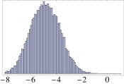
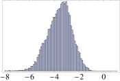
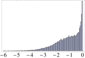
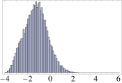
$\log\lambda_{u}$ [$-5.5$]	$\log\lambda_{d,e}$ [$-5.2,-5.5$]	$\log(2\theta^{\rm CKM}_{12}/\pi)$ [$-0.8$]	$\log C^{\nu}_{1}$
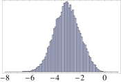
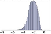
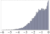
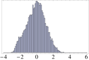
$\log\lambda_{c}$ [$-2.9$]	$\log\lambda_{s,\mu}$ [$-3.9,-3.2$]	$\log(2\theta^{\rm CKM}_{23}/\pi)$ [$-1.6$]	$\log C^{\nu}_{2}$
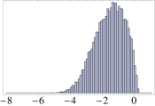
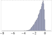
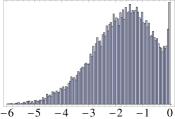
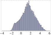
$\log\lambda_{t}$ [$-0.3$]	$\log\lambda_{b,\tau}$ [$-2.2,-2.0$]	$\log\sin(\theta^{\rm CKM}_{13})$ [$-2.4$]	$\log C^{\nu}_{3}$
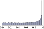
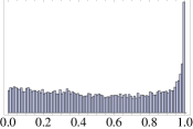
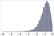
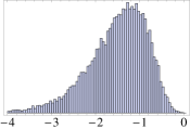
$\sin(2\theta^{\rm PMNS}_{12})$ [$0.92\pm 0.01$]	$\sin(2\theta^{\rm PMNS}_{23})$ [$>0.96$]	$\log\sin(\theta^{\rm PMNS}_{13})$ [$<-0.74$]	$\log(m^{\nu}_{2}/m^{\nu}_{3})$ [$-0.75\pm 0.05$]

Figure 1: Distributions of flavor observables for the Gaussian landscape on $T^{2}$. We set $p(y)=1$, $r_{a}=0$ for all $a$, $g_{\rm eff}=0.5$, $d/L=0.1$, $d_{\rm\bar{5}}/L=0.3$, and assume $N_{n}=20$ right-handed neutrinos. All logarithms are base ten, $\lambda_{a}$ denotes the Yukawa coupling determining the mass of particle $a$, and $C^{\nu}_{i}$ is the $i$th eigenvalue of the low-energy neutrino mass matrix $C^{\nu}$; other notations conform to those of the Particle Data Group. The scale $\left\langle{\phi}\right\rangle$ has been set so that the median of $C^{\nu}_{2}$ is one. The numbers in brackets represent experimental values PDG , run up to the Planck scale. See the main text for details.

As we have already described, the peak positions $y^{a_{i}}$ are taken to scan randomly and independently over the interval $[0,L]$. Although there are 22 flavor observables, for $D\geq 2$ the number of scanning parameters exceeds this, and the Gaussian landscape makes no “hard” predictions. Instead, one obtains (correlated) probability distributions for the flavor observables. These are reflected in the binned results of a numerical simulation, displayed in Fig. 1. For reference, Fig. 1 also gives experimental values in brackets. These have been obtained by using renormalization group flow to run Particle Data Group PDG mean values or constraints up to the Planck scale, where, for concreteness, we assume no particle content beyond the Standard Model and ignore the effect of the right-handed neutrinos (alternatively, one could extend the Gaussian landscape to cover low-energy supersymmetry). We here emphasize that Fig. 1 displays the statistical distributions of flavor observables among vacua in the Gaussian landscape, and does not include cosmological or anthropic selection effects, the latter of which we anticipate would modulate at least the distributions of $\lambda_{u,d,e}$.

The distributions in Fig. 1 are all quite broad. This is undesirable, from the point of view of experimental verification, but may be the reality of flavor in the landscape. Although the distributions are broad, the observed patterns among flavor parameters are present. For example, although the distributions of quark and charged lepton masses have considerable overlap within any given family, correlations among these masses are such that they are typically hierarchically separated. Furthermore, quark mixing angles are typically small, and $\theta^{\rm CKM}_{13}$ tends to be smaller than the others. It should be emphasized that the mass hierarchies and small mixing angles of the quark sector exhibit both the pairing structure and generation structure of the Standard Model, whereas neither of these is input directly into the Gaussian landscape.

Note that the distribution of the $d$ quark Yukawa coupling (and that of the electron) does not range over such small values as that of the $u$ quark. This reflects a reduced hierarchy, which is a consequence of the broader widths assigned to the down-type quarks (lepton doublets). If down-type quarks were assigned width $d$, their distributions would match those of up-type quarks. As they are, the distributions do not provide a bad fit to observation. However, if we consider an extension of the Gaussian landscape to include low-energy supersymmetry breaking, then $\tan\beta\sim{\mathcal{O}}(10)$ would seem to provide an improved statistical fit. Further investigation of this possibility is beyond the scope of this work. See also footnote 4.

The mechanism that generates small mixing angles in the quark sector—which stems from the up-type and down-type Yukawa overlaps sharing the localized wavefunctions of the quark doublets and Higgs boson—fails in the lepton sector, due to the broad widths of the lepton doublet wavefunctions. Ref. HSW2 found that broad-width lepton doublets to be necessary but insufficient: without large CP-violating phases $r_{a}$ the relevant terms contributing to the PMNS matrix canceled. We find, however, that large CP-violating phases are unnecessary if the kinetic terms $K^{a}_{ij}$ are determined by overlap integration, as in Eq. (9). The distributions of lepton mixing angles are broad, even with $r=0$, so long as $d_{\ell}/L\gtrsim 0.3$.

Ref. HSW2 found low-energy neutrinos to exhibit enormous mass hierarchy when $N_{n}=3$. This hierarchy ultimately stems from rank reduction in the mass matrix $C^{\nu}$, which has the effect of “adding” the hierarchies among the eigenvalues of $\lambda^{n}$ to those of $\lambda^{M}$. Qualitatively, the low-energy neutrino mass hierarchy is related to the hierarchy among the three largest values of $\lambda_{n_{i}}^{2}/\lambda_{M_{i}}$, where $\lambda_{n_{i}}$ and $\lambda_{M_{i}}$ denote respectively the eigenvalues of $\lambda^{n}$ and $\lambda^{M}$. When $N_{n}=3$, the hierarchy among these terms is quite large. However, a consequence of choosing a large number of right-handed neutrinos, $N_{n}\gg 3$, is their mass eigenvalues become densely packed. This is not hard to understand: the overall range of hierarchy is proportional to $(L/d_{n})^{2}$, and as more masses are inserted in this range their typical separation decreases. In turn, the three largest values of $\lambda_{n_{i}}^{2}/\lambda_{M_{i}}$ exhibit reduced hierarchy as $N_{n}$ is increased. Indeed, we see in Fig. 1 that the hierarchy among low-energy neutrino masses is not much larger than that among the quarks and charged leptons.

Furthermore, it seems correlations tend to prevent the low-energy neutrino mass hierarchy from becoming too large in any given vacuum. As an example of this, in Fig. 1 we display the distribution of (the logarithm of) $m^{\nu}_{2}/m^{\nu}_{3}$, the ratio of the middle to the most massive low-energy neutrino. We see that typically $m^{\nu}_{3}$ is not much more than 10–100 times larger than $m^{\nu}_{2}$. Note that, in the limit of hierarchical low-energy neutrino masses,

$$\sqrt{\Delta m^{2}_{\odot}/\Delta m^{2}_{\rm atm}}\simeq m^{\nu}_{2}/m^{\nu}_{3}\,.$$ (12)

Hence in Fig. 1 we provide the observational constraint on the ratio of $\Delta m^{2}$ of solar to atmospheric neutrino oscillations. The Gaussian landscape provides a reasonable fit to this observation.

Fig. 1 refers to a specific choice of right-handed neutrino wavefunction widths $d_{n}$, as well as that of the symmetry-breaking field(s) $d_{\phi}$. However, we have performed numerical simulations like that above but with $d_{n}/L=0.3$ or $d_{\phi}/L=0.3$, and have found that when $D\geq 2$ and $N_{n}\gg 3$ the distributions of flavor observables are qualitatively unchanged from those in Fig. 1. It should be noted that choosing $N_{n}=3$ increases the sensitivity of flavor observables to the distribution of right-handed neutrino masses, so that $m^{\nu}_{2}/m^{\nu}_{3}$ becomes sensitive to $d_{n}$. A larger low-energy neutrino mass hierarchy becomes more likely in this case, with the best fit to observation coming from choosing narrow $d_{n}$.

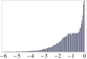
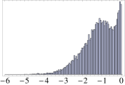
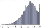
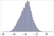
$\log(2\theta^{\rm CKM}_{12}/\pi)$ [$-0.8$]	$\log(2\theta^{\rm CKM}_{23}/\pi)$ [$-1.6$]	$\log\sin(\theta^{\rm CKM}_{13})$ [$-2.4$]	$\log\lambda_{d,e}$ [$-5.2,-5.5$]
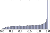
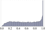
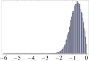
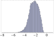
$\sin(2\theta^{\rm PMNS}_{12})$ [0.91–0.93]	$\sin(2\theta^{\rm PMNS}_{23})$ [$>0.96$]	$\log\sin(\theta^{\rm PMNS}_{13})$ [$<-0.74$]	$\log\lambda_{s,\mu}$ [$-3.9,-3.2$]
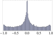
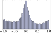
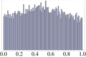
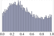
$\delta^{\rm CKM}/\pi$ [0.29–0.34]	$\delta^{\rm PMNS}/\pi$	$\alpha_{1}/\pi$	$\alpha_{2}/\pi$

Figure 2: Distributions of flavor observables for the Gaussian landscape on $T^{2}$. Notation and parameters are as in Fig. 1, except $r=0.3$. Distributions of flavor observables that are not displayed above are essentially unchanged from when $r=0$.

Let us now discuss CP violation in the Gaussian landscape. As has already been remarked, it is unclear how CP violation should be introduced into the Gaussian landscape in order to best reflect the phenomenology of string compactification. We have explored the two most obvious choices—using a $\Gamma$-matrix phase function $p(y)$ or wavefunction phases $r_{a}$—and, remarkably, have found that both leave the distributions of CP-conserving observables qualitatively intact. Furthermore, at least for the simple cases we have considered, both give similar predictions for the distributions of CP-violating phases.

For illustration, in Fig. 2 we display results of a numerical simulation exactly like that behind Fig. 1, but using $r_{a}=r=0.3$ for all $a$ (we study uniform $r_{a}=r$ merely for simplicity). Some CP-conserving flavor observables are not displayed in Fig. 2 because we could not detect any changes in their distributions relative to Fig. 1. Those observables for which we could detect changes are displayed in the top two rows of Fig. 2. It is seen that these changes are not very significant, considering that our universe provides only one data point to sample each distribution. The four CP-violating phases are displayed in the bottom row. Although the distribution of $\delta^{\rm CKM}$ is peaked at zero, the value we observe does not appear atypical. Both increasing and decreasing $r$ from $r=0.3$ tends to sharpen the peak at $\delta^{\rm CKM}=0$, the effect being rather mild for increasing $r$. (Increasing $r$ also tends to broaden the distributions of the quark mixing angles and of the mass eigenvalues $\lambda_{d_{i},e_{i}}$, while at the same time pushing their medians to smaller values.)

We have also performed a numerical simulation using $r=0$, $p(y)=e^{2\pi i(y_{1}+y_{2})/L}$ (for clarity we make explicit the two coordinates $y_{1}$ and $y_{2}$ of the internal manifold $T^{2}$). The resulting distributions are almost indistinguishable from those obtained by choosing $r=0.3$, $p(y)=1$ (Fig. 2), except for the distributions of $\alpha_{1}$ and $\alpha_{2}$, which are completely flat, and those of some CP-conserving observables, which more closely resemble the distributions in Fig. 1.

IV The AFS Approximation

Although computations involving overlap integrations, diagonalizing mass matrices, etc., are most conveniently carried out numerically, it is possible to understand analytically the qualitative features of the distributions of various flavor observables in Gaussian landscapes. Such an understanding develops intuition for how these distributions depend on the values of parameters that were taken as given in the numerical simulations of Section III, and thus allows us to anticipate the results of other choices of parameters without having to repeat the numerical simulation. Furthermore, as was seen in Ref. HSW2 , such an analysis can reveal how the distributions of flavor observables are related to various features of the geometry of compactification. Thus, we here extend the analysis of Ref. HSW2 by taking account of the kinetic mixing in the $K^{a}_{ij}$ matrices.

In Ref. HSW2 , the present authors found that the distributions of Yukawa couplings in Gaussian landscapes (using the basis of zero modes explored there) are almost the same as those predicted by models with approximate abelian flavor symmetries (AFS). In the AFS approach to flavor FN , one assumes each of the Standard–Model fermions has its own U(1) charge. If the $i$th anti-up quark has a U(1) charge $a_{i}\geq 0$, the $j$th left-handed quark doublet has a charge $b_{j}\geq 0$, and the Higgs boson is neutral under the U(1) symmetry, then their Yukawa coupling is

$$\lambda^{u}_{ij}=g_{ij}\epsilon^{a_{i}}\epsilon^{b_{j}}\,,$$ (13)

where the small parameter $\epsilon\ll 1$ comes from a small breaking of the U(1) symmetry, and the $g_{ij}$ are coefficients of order unity, presumably determined by a higher-energy theory. Ref. HSW2 showed that Yukawa couplings have the same structure in Gaussian landscapes, when the small suppression factors $\epsilon^{a_{i}}$ and $\epsilon^{b_{j}}$ are interpreted properly, even though there is no approximately preserved U(1) flavor symmetry. This allows for a simple analytic understanding of quark and lepton masses and mixings. Below we show that a similar analytic understanding of the predictions of Gaussian landscapes is possible when including non-trivial kinetic mixing $K^{a}_{ij}$ and increasing the number of right-handed neutrinos.

To proceed, we introduce a series of simplifying approximations HSW2 . First, we ignore the fact that $B$ is a compact manifold and instead treat it like Euclidian space $\mathbb{R}^{D}$ when calculating overlap integrals. This approximation becomes more accurate in the limit where wavefunctions are peaked nearer to each other—i.e. when the Yukawa couplings become large—but is surprisingly effective at describing the qualitative shapes of distributions of Yukawa matrix elements, as was confirmed by a number of numerical simulations in Ref. HSW2 . Furthermore, for simplicity we set $p(y)=1$ and $r_{a}=0$ (recall that the CP-conserving observables are approximately independent of the $r_{a}$ when $r_{a}\lesssim 0.3$).

With these approximations, the relevant overlap integrals have simple analytic expressions. For example, the up-type Yukawa matrix is given by

$$\lambda^{u}_{ij}\sim\exp\!\left[-\frac{y_{u_{i}}^{2}+y_{q_{j}}^{2}-y^{u_{i}}y^{q_{j}}}{3d^{2}}\right],$$ (14)

where we have used translational invariance over the extra-dimensional space $\mathbb{R}^{D}$ (this is true in $T^{D}$ as well) to set $y^{h}=0$. Note that for $D>1$, the $y^{a_{i}}$ are vectors on the space of extra dimensions, and terms like $y^{a_{i}}y^{b_{j}}$ correspond to scalar products of vectors. The last term in the exponent is “statistically neutral;” that is, it is linear in the random peak positions $y^{u_{i}}$ and $y^{q_{j}}$, and therefore can be positive or negative, with a contribution that largely cancels in the statistical distribution.

The up-type Yukawa matrix has the AFS structure,

$$\lambda^{u}_{ij}\sim g_{ij}\epsilon^{u}_{i}\epsilon^{q}_{j},$$ (15)

where the small factors $\epsilon^{u}_{i}$ and $\epsilon^{q}_{j}$ correspond to the first two terms in the exponent of $\lambda^{u}_{ij}$ in Eq. (14), while the $g_{ij}$ comes from the third term. Again, the $g_{ij}$ are random numbers that may be larger or smaller than unity, but are statistically neutral. We can always relabel the generation index $i$ of the three independent anti-up-type quarks $\bar{u}_{i}$, so that $\epsilon^{u}_{1}<\epsilon^{u}_{2}<\epsilon^{u}_{3}$. Similarly, the generation index for the three quark doublets can be relabeled, so that $\epsilon^{q}_{1}<\epsilon^{q}_{2}<\epsilon^{q}_{3}$. Note that in approximate AFS models, $\epsilon$ is a fixed-value symmetry-breaking parameter, and the U(1) charge assignments $a_{i}$ and $b_{j}$ are picked “by hand,” whereas in Gaussian landscapes the “AFS factors” $\epsilon^{u}_{1}<\epsilon^{u}_{2}<\epsilon^{u}_{3}$ and $\epsilon^{q}_{1}<\epsilon^{q}_{2}<\epsilon^{q}_{3}$ follow statistical distributions. The quantity $(L/d)^{2}$ sets the order-of-magnitude of hierarchy in Gaussian landscapes, $\lambda\sim e^{-(L/d)^{2}}$, playing a role analogous to the symmetry-breaking parameter $\epsilon$ in approximate AFS models.

For relevance to the results of Section III, we assume the down-type quark wavefunctions have a relatively broad width $d_{\bf\bar{5}}\sim{\mathcal{O}}(L)$, while all other fields have the same (narrow) width $d\ll L$. The down-type Yukawa matrix then has the structure

$$\lambda^{d}_{ij}\sim\varphi^{d}_{i}|_{y=y^{q_{j}}\!/2}\,\left(\epsilon^{q}_{j}\right)^{\frac{3}{4}}.$$ (16)

The broad-width wavefunctions $\varphi^{d}_{i}$ are simply evaluated at the peak of the overlap, which occurs between the localization of the Higgs boson $y=y^{h}=0$ and that of the quark-doublet wavefunctions $y=y^{q_{j}}$, and can be seen to introduce a set of random numbers of order the down-type wavefunction normalization. Thus, the down-type Yukawa matrix $\lambda^{d}_{ij}$ also follows the structure of approximate AFS models.

So far, our discussion has mirrored that of Refs. HSW1 ; HSW2 . However, that work ignored the effect of kinetic mixing. Applying the approximations described above, the kinetic mixing of quarks is given by

$$K^{a}_{ij}\sim\exp\!\left[-\frac{1}{4d^{2}}\left(y^{a_{i}}-y^{a_{j}}\right)^{2}\right]\,,$$ (17)

for $a=u,d,q$. Such a kinetic matrix can be put in canonical form by rotating quark flavors using a “triangular” matrix, for example the quark doublets are made canonical (with an appropriate normalization of $\varphi^{q}_{i}$) by

$$\left(\begin{array}[]{c}q_{1}\\ q_{2}\\ q_{3}\end{array}\right)\sim\left(\begin{array}[]{ccc}1&-K^{q}_{12}&-K^{q}_{13}\\ 0&1&-K^{q}_{23}\\ 0&0&1\end{array}\right)\left(\begin{array}[]{c}q^{\prime}_{1}\\ q^{\prime}_{2}\\ q^{\prime}_{3}\end{array}\right)\,.$$ (27)

In the above, we have kept only leading order terms; note $K^{q}_{ij}$ is of order $(\epsilon^{q}_{i}\epsilon^{q}_{j})^{\frac{3}{4}}$ for $i\neq j$ and thus the off-diagonal terms are small compared to unity. An analogous expression applies to the up-type quarks. The down-type kinetic matrices do not necessarily have small off-diagonal terms, yet they can be put in canonical form via a matrix of such “triangular” form.

Note that these rotations do not affect the AFS structure of the quark Yukawa couplings. The off-diagonal terms in the “triangular” rotation matrices for up-type quarks and quark doublets are negligible in this qualitative analysis, and so $\lambda^{u}$ retains the structure of Eq. (15). Meanwhile, the “triangular” form of the down-type quark rotation essentially replaces the random terms $\varphi^{d}_{i}|_{y=y^{q_{j}}/2}$ with linear combinations of such terms—this does not change the structure of $\lambda^{d}$. Thus, the quark sector of the Gaussian landscape retains its AFS structure. It is straightforward to see that the Yukawa eigenvalues are roughly given by $\epsilon^{u}_{i}\epsilon^{q}_{i}$ ($i=1,2,3$), and $(\epsilon^{q}_{j})^{\frac{3}{4}}$ ($j=1,2,3$), in the up-type and down-type sectors, respectively.

As has been mentioned, the AFS factors $\epsilon^{u}_{i}$ and $\epsilon^{q}_{j}$ are described by correlated statistical distributions reflecting the random scanning of Gaussian wavefunction peak positions. Their statistical distributions encapsulate the hierarchical suppression that must be inserted “by hand” using U(1) flavor charges in AFS models. Ref. HSW2 explains how the geometry of $B$ affects the distributions of the AFS factors. That analysis carries over directly to the Gaussian landscapes considered here, so for brevity we do not repeat it. Instead, we simply note that distributions of flavor observables are qualitatively independent the geometry of the internal manifold.

Let us now turn to quark-sector electroweak mixing. Keeping in mind that kinetic mixing does not change the structures of $\lambda^{u}$ and $\lambda^{d}$ in Eqs. (15) and (16), the CKM mixing angles are given by the difference between the diagonalization angles $\theta_{ij}\sim\epsilon^{q}_{i}/\epsilon^{q}_{j}$ ($i<j$) for the up-type Yukawa matrix and $\theta_{ij}\sim(\epsilon^{q}_{i}/\epsilon^{q}_{j})^{\frac{3}{4}}$ ($i<j$) for the down-type Yukawa matrix. Qualitatively, the difference is dominated by the larger mixing angle, and hence

$$\theta^{\rm CKM}_{ij}\sim(\epsilon^{q}_{i}/\epsilon^{q}_{j})^{\frac{3}{4}}\sim\lambda_{d_{i}}/\lambda_{d_{j}}\sim(\lambda_{u_{i}}/\lambda_{u_{j}})^{\frac{3}{8}}\,.$$ (28)

The last two expressions relate the typical size of CKM mixing angles to typical ratios of quark mass eigenvalues, due to all of these observables being qualitatively determined by the same AFS factors.

The lepton sector can be analyzed similarly. Now the lepton doublet has broad width $d_{\bf\bar{5}}$, while the other zero modes have narrow wavefunctions. Thus, the charged-lepton and neutrino Yukawa matrices have the structure

$$\lambda^{e}_{ij} \sim (\epsilon^{e}_{i})^{\frac{3}{4}}\,\varphi^{\ell}_{j}|_{y=y^{e_{i}}\!/2}$$ (29)

$$\lambda^{n}_{ij} \sim (\epsilon^{n}_{i})^{\frac{3}{4}}\,\varphi^{\ell}_{j}|_{y=y^{n_{i}}\!/2}\,.$$ (30)

These matrices have essentially the same structure as $\lambda^{d}_{ij}$. Likewise, kinetic mixing in the lepton sector is either negligible (for electroweak singlets) or simply mixes the random factors $\varphi^{\ell}_{j}$. Hence, the mass eigenvalues in the charged-lepton sector are qualitatively given by $(\epsilon^{e}_{1})^{\frac{3}{4}}$, $(\epsilon^{e}_{2})^{\frac{3}{4}}$, and $(\epsilon^{e}_{3})^{\frac{3}{4}}$, where again we relabel generation indices so that $\epsilon^{e}_{1}<\epsilon^{e}_{2}<\epsilon^{e}_{3}$. Their distributions are the same as those of the down-type quarks.

Because the right-handed neutrino mass matrix $\lambda^{M}$ involves the overlap of two right-handed neutrinos, it is well approximated as a diagonal matrix,

$$\lambda^{M}_{ij}\sim\epsilon^{M}_{i}\delta_{ij}\,.$$ (31)

The diagonal elements $\epsilon^{M}_{i}$ may be small due to small right-handed neutrino overlap with the symmetry-breaking field $\phi$. The seesaw mass matrix of left-handed neutrinos then takes the form

$$C_{ij}\sim\sum_{k=1}^{N_{n}}\varphi^{\ell}_{i}|_{y=y^{n_{k}}\!/2}\,\,\varphi^{\ell}_{j}|_{y=y^{n_{k}}\!/2}\,(\epsilon^{n}_{k})^{\frac{3}{2}}\!/\epsilon^{M}_{k}\,.$$ (32)

The distribution of AFS factors $\epsilon^{n}_{k}\sim e^{-(y^{n_{k}})^{2}\!/3d^{2}}$ covers a logarithmic range proportional to $(L/d)^{2}$. If, as we have assumed, the Majorana mass matrix $\lambda^{M}_{ij}$ is determined by overlap integration of right-handed neutrinos with a Gaussian wavefunction for $\phi$, then the diagonal elements $\epsilon^{M}_{i}$ are also distributed over a logarithmic range proportional to $(L/d)^{2}$. The seesaw mass matrix $C_{ij}$ involves summation over all right-handed neutrinos, but its three eigenvalues are essentially determined by the contributions with the three largest values of $c_{k}\equiv(\epsilon^{n}_{k})^{\frac{3}{2}}\!/\epsilon^{M}_{k}$. Although collectively the $N_{n}$ individual $c_{k}$ range over a logarithmic scale proportional to $(L/d)^{2}$, the three largest values strongly depend on $N_{n}$. As the number of right-handed neutrinos $N_{n}$ is increased, typically the three largest values of $c_{k}$ will become bunched near the largest possible value of $c_{k}$. In turn, the three eigenvalues of $C_{ij}$ experience reduced hierarchy as $N_{n}$ is increased. This is in good agreement with the measured ratio of $\Delta m^{2}$ coming from solar and atmospheric neutrino oscillations.

Finally, we consider the distributions of the PMNS mixing angles. Because the different elements of a given row of $\lambda^{e}$ and $C$ are comparable to each other (due to broad-width lepton doublet wavefunctions), large-angle left-side rotations are necessary to diagonalize these matrices. Naively, these large-angle rotations would correspond to large PMNS mixing angles. However, the present authors concluded in Ref. HSW2 (where kinetic mixing was ignored) that broad-width lepton doublet wavefunctions are insufficient to generate large PMNS mixing angles. The reason is, the broad-width wavefunctions $\varphi^{\ell}_{j}(y)$ are not very different for different zero modes (different $j$). As a result, the diagonalization angles for the left-handed charged leptons and those for the left-handed neutrinos are highly constrained, and an accidental cancellation occurs in the PMNS matrix. Thus, it was concluded that some other ingredient(s)—such as large CP-violating phases—must be included in order for large lepton mixing to be typical in Gaussian landscapes.

However, Ref. HSW2 ignored kinetic mixing. As has been remarked, rotating leptons to a canonical basis of zero modes does not change the qualitative structure of the Yukawa matrices $\lambda^{e}$ and $\lambda^{n}$, nor the mass matrices $\lambda^{M}$ and $C$. However, in such a basis the three independent zero modes of each family are orthogonal to one another, which is quite unlike the situation imagined in Ref. HSW2 , where these zero modes were rather homogeneous and similar. The effect of this is to prevent the accidental cancellation that was observed in Ref. HSW2 . Thus, PMNS mixing angles obtain their “naive” values, comparable to ratios of different elements in a given row of $\lambda^{e}$ or $\lambda^{n}$, which are typically order unity. Numerical simulations in Section III confirm this idea.

V Conclusions

The idea that characteristics of our universe are selected from a landscape of vacua has proved quite provocative. The major criticisms of this hypothesis can be classified into three groups: $i$) the landscape combined with eternal inflation implies a multiverse with diverging spacetime volume, expectations for observables depend on how this diverging volume is regulated, yet it is unclear how this should be done; $ii$) expectations for observables depend on anthropic selection effects, however it is unclear how to define our reference class, and at the same time the calculation of anthropic effects tends to be very complicated; and $iii$) our universe provides only one data point to compare to the predicted distribution of each scanning parameter, making landscape models seem difficult to falsify.

On the other hand, the flavor physics of a landscape tends to avoid each of these criticisms. Although the cosmology of eternal inflation and the spacetime measure of the multiverse ($i$) strongly influence the distributions of cosmological observables such as the observed primordial cosmic density contrast, insofar as the landscape is large enough that low-energy physics is decoupled from inflationary dynamics, flavor physics should be independent of these issues. Furthermore, although it is expected that anthropic selection ($ii$) plays an important role in determining some flavor parameters, such as the $u$, $d$, and $e$ masses, most flavor parameters seem decoupled from conditions necessary to allow for the evolution of observers. Finally, although we have only one universe in which we can perform measurements ($iii$), there are almost two dozen (possibly correlated) flavor observables that should be described by the landscape model, allowing for a more discerning statistical analysis. Thus, we consider the issue of flavor to be ideal for applying the landscape hypothesis.

- (1) L. J. Hall, H. Murayama and N. Weiner, “Neutrino mass anarchy,” Phys. Rev. Lett. 84, 2572 (2000) [arXiv:hep-ph/9911341].
- (2) J. F. Donoghue, K. Dutta and A. Ross, “Quark and lepton masses and mixing in the landscape,” Phys. Rev. D 73, 113002 (2006) [arXiv:hep-ph/0511219].
- (3) L. J. Hall, M. P. Salem and T. Watari, “Quark and Lepton Masses from Gaussian Landscapes,” Phys. Rev. Lett. 100, 141801 (2008) [arXiv:0707.3444 [hep-ph]].
- (4) L. J. Hall, M. P. Salem and T. Watari, “Statistical Understanding of Quark and Lepton Masses in Gaussian Landscapes,” Phys. Rev. D 76, 093001 (2007) [arXiv:0707.3446 [hep-ph]].
- (5) M. Grana, “Flux compactifications in string theory: A comprehensive review,” Phys. Rept. 423, 91 (2006) [arXiv:hep-th/0509003]; M. R. Douglas and S. Kachru, “Flux compactification,” Rev. Mod. Phys. 79, 733 (2007) [arXiv:hep-th/0610102]; F. Denef, “Les Houches Lectures on Constructing String Vacua,” arXiv:0803.1194 [hep-th].
- (6) N. Arkani-Hamed and M. Schmaltz, “Hierarchies without symmetries from extra dimensions,” Phys. Rev. D 61, 033005 (2000) [arXiv:hep-ph/9903417].
- (7) R. Friedman, J. Morgan and E. Witten, “Vector bundles and F theory,” Commun. Math. Phys. 187, 679 (1997) [arXiv:hep-th/9701162]; B. Acharya and E. Witten, “Chiral fermions from manifolds of G(2) holonomy,” arXiv:hep-th/0109152. See also S. H. Katz and C. Vafa, “Matter from geometry,” Nucl. Phys. B 497, 146 (1997) [arXiv:hep-th/9606086].
- (8) L. J. Hall and Y. Nomura, “Gauge unification in higher dimensions,” Phys. Rev. D 64, 055003 (2001) [arXiv:hep-ph/0103125]; R. Tatar and T. Watari, “GUT Relations from String Theory Compactifications,” arXiv:0806.0634 [hep-th].
- (9) M. R. Douglas, R. L. Karp, S. Lukic and R. Reinbacher, “Numerical solution to the hermitian Yang-Mills equation on the Fermat quintic,” JHEP 0712, 083 (2007) [arXiv:hep-th/0606261]; M. R. Douglas, R. L. Karp, S. Lukic and R. Reinbacher, “Numerical Calabi-Yau metrics,” J. Math. Phys. 49, 032302 (2008) [arXiv:hep-th/0612075]; V. Braun, T. Brelidze, M. R. Douglas and B. A. Ovrut, “Calabi-Yau Metrics for Quotients and Complete Intersections,” JHEP 0805, 080 (2008) [arXiv:0712.3563 [hep-th]].
- (10) J. F. Donoghue, “The fine-tuning problems of particle physics and anthropic mechanisms,” arXiv:0710.4080 [hep-ph]; L. J. Hall and Y. Nomura, “Evidence for the Multiverse in the Standard Model and Beyond,” Phys. Rev. D 78, 035001 (2008) [arXiv:0712.2454 [hep-ph]]; R. L. Jaffe, A. Jenkins and I. Kimchi, “Quark Masses: An Environmental Impact Statement,” arXiv:0809.1647 [hep-ph].
- (11) W. M. Yao et al. [Particle Data Group], “Review of particle physics,” J. Phys. G 33, 1 (2006).
- (12) C. D. Froggatt and H. B. Nielsen, “Hierarchy Of Quark Masses, Cabibbo Angles And CP Violation,” Nucl. Phys. B 147, 277 (1979).