$\Lambda$CDM predictions for galaxy protoclusters I: The relation between galaxies, protoclusters and quasars at $z\sim 6$

Abstract

Motivated by recent observational studies of the environment of $z\sim 6$ QSOs, we have used the Millennium Run (MR) simulations to construct a very large ($\sim 4\degr\times 4\degr$) mock redshift survey of star-forming galaxies at $z\sim 6$. We use this simulated survey to study the relation between density enhancements in the distribution of $i_{775}$-dropouts and Ly$\alpha$ emitters, and their relation to the most massive halos and protocluster regions at $z\sim 6$. Our simulation predicts significant variations in surface density across the sky with some voids and filaments extending over scales of 1$\degr$, much larger than probed by current surveys. Approximately one third of all $z\sim 6$ halos hosting $i$-dropouts brighter than $z$=26.5 mag ($\approx M^{*}_{UV,z=6}$) become part of $z=0$ galaxy clusters. $i$-dropouts associated with protocluster regions are found in regions where the surface density is enhanced on scales ranging from a few to several tens of arcminutes on the sky. We analyze two structures of $i$-dropouts and Ly$\alpha$ emitters observed with the Subaru Telescope and show that these structures must be the seeds of massive clusters-in-formation. In striking contrast, six $z\sim 6$ QSO fields observed with HST show no significant enhancements in their $i_{775}$-dropout number counts. With the present data, we cannot rule out the QSOs being hosted by the most massive halos. However, neither can we confirm this widely used assumption. We conclude by giving detailed recommendations for the interpretation and planning of observations by current and future ground- and space based instruments that will shed new light on questions related to the large-scale structure at $z\sim 6$.

1 Introduction

During the first decade of the third Millennium we have begun to put observational constraints on the status quo of galaxy formation at roughly one billion years after the Big Bang (e.g. Stanway et al., 2003; Yan & Windhorst, 2004a; Bouwens et al., 2003, 2004a, 2006; Dickinson et al., 2004; Malhotra et al., 2005; Shimasaku et al., 2005; Ouchi et al., 2005; Overzier et al., 2006). Statistical samples of star-forming galaxies at $z=6$ – either selected on the basis of their large (i–z) color due to the Lyman break redshifted to $z\sim 6$ (i-dropouts), or on the basis of the large equivalent width of Ly$\alpha$ emission (Ly$\alpha$ emitters) – suggest that they are analogous to the population of Lyman break galaxies (LBGs) found at $z\sim 3-5$ (e.g. Bouwens et al., 2007). A small subset of the $i_{775}$-dropouts has been found to be surprisingly massive or old (Dow-Hygelund et al., 2005; Yan et al., 2006; Eyles et al., 2007). The slope of the UV luminosity function at $z=6$ is very steep and implies that low luminosity objects contributed significantly to reionizing the Universe (Yan & Windhorst, 2004b; Bouwens et al., 2007; Khochfar et al., 2007; Overzier et al., 2008a). Cosmological hydrodynamic simulations are being used to reproduce the abundances as well as the spectral energy distributions of $z=6$ galaxies. Exactly how these objects are connected to local galaxies remains a highly active area of research (e.g. Davé et al., 2006; Gayler Harford & Gnedin, 2006; Nagamine et al., 2006, 2008; Night et al., 2006; Finlator et al., 2007; Robertson et al., 2007).

The discovery of highly luminous quasi-stellar objects (QSOs) at $z\sim 6$ (e.g. Fan et al., 2001, 2003, 2004, 2006a; Goto, 2006; Venemans et al., 2007) is of equal importance in our understanding of the formation of the first massive black holes and galaxies. Gunn & Peterson (1965) absorption troughs in their spectra demarcate the end of the epoch of reionization (e.g. Fan et al., 2001; White et al., 2003; Walter et al., 2004; Fan et al., 2006b). Assuming that high redshift QSOs are radiating near the Eddington limit, they contain supermassive black holes (SMBHs) of mass $\sim 10^{9}$ $M_{\odot}$ (e.g. Willott et al., 2003; Barth et al., 2003; Vestergaard, 2004; Jiang et al., 2007; Kurk et al., 2007). The spectral properties of most $z\sim 6$ QSOs in the rest-frame UV, optical, IR and X-ray are similar to those at low redshift, suggesting that massive, and highly chemically enriched galaxies were vigorously forming stars and SMBHs less than one billion years after the Big Bang (e.g. Bertoldi et al., 2003; Maiolino et al., 2005; Jiang et al., 2006; Wang et al., 2007).

Hierarchical formation models and simulations can reproduce the existence of such massive objects at early times (e.g. Haiman & Loeb, 2001; Springel et al., 2005a; Begelman et al., 2006; Volonteri & Rees, 2006; Li et al., 2007; Narayanan et al., 2007), provided however that they are situated in extremely massive halos. Large-scale gravitational clustering is a powerful method for estimating halo masses of quasars at low redshifts, but cannot be applied to $z\sim 6$ QSOs because there are too few systems known. Their extremely low space density determined from the Sloan Digital Sky Survey (SDSS) of $\sim$1 Gpc^-3 (comoving) implies a (maximum) halo mass of $\cal{M}$${}_{halo}\sim 10^{13}$ $M_{\odot}$ (Fan et al., 2001; Li et al., 2007). A similar halo mass is obtained when extrapolating from the ($z=0$) relationship between black hole mass and bulge mass of Magorrian et al. (1998), and using $\Omega_{M}/\Omega_{bar}\gtrsim 10$ (Fan et al., 2001). Because the descendants of the most massive halos at $z\sim 6$ may evolve into halos of $>10^{15}$ $M_{\odot}$ at $z=0$ in a $\Lambda$CDM model, (e.g. Springel et al., 2005a; Suwa et al., 2006; Li et al., 2007, but see De Lucia & Blaizot (2007), Trenti et al. (2008) and Sect. 5 of this paper), it is believed that the QSOs trace highly biased regions that may give birth to the most massive present-day galaxy clusters. If this is true, the small-scale environment of $z\sim 6$ QSOs may be expected to show a significant enhancement in the number of small, faint galaxies. These galaxies may either merge with the QSO host galaxy, or may form the first stars and black holes of other (proto-)cluster galaxies.

Observations carried out with the Advanced Camera for Surveys (ACS) on the Hubble Space Telescope (HST), allowed a rough measurement of the two-dimensional overdensities of faint $i_{775}$-dopouts detected towards the QSOs J0836+0054 at $z=5.8$ (Zheng et al., 2006) and J1030+0524 at $z=6.28$ (Stiavelli et al., 2005). Recently Kim et al. (2008) presented results from a sample of 5 QSO fields, finding some to be overdense and some to be underdense with respect to the HST/ACS Great Observatories Origins Deep Survey (GOODS). Priddey et al. (2007) find enhancements in the number counts of sub-mm galaxies. Substantial overdensities of $i$-dropouts and Ly$\alpha$ emitters have also been found in non-QSO fields (e.g. Shimasaku et al., 2003; Ouchi et al., 2005; Ota et al., 2008), suggesting that massive structures do not always harbour a QSO, which may be explained by invoking a QSO duty-cycle. At $z\sim 2-5$, significant excesses of star-forming galaxies have been found near QSOs (e.g. Djorgovski et al., 2003; Kashikawa et al., 2007), radio galaxies (e.g. Miley et al., 2004; Venemans et al., 2007; Overzier et al., 2008b), and in random fields (Steidel et al., 1998, 2005). Although the physical interpretation of the measurements is uncertain, these structures are believed to be associated with the formation of clusters of galaxies.

The idea of verifying the presence of massive structures at high redshift through the clustering of small galaxies around them has recently been explored by, e.g., Muñoz & Loeb (2008a) using the excursion set formalism of halo growth (Zentner, 2007). However, the direct comparison between models or simulations and observations remains difficult, mainly because of complicated observational selection effects. This is especially true at high redshift. In order to investigate how a wide variety of galaxy overdensities found in surveys at $z\simeq 2-6$ are related to cluster formation, we have carried out an analysis of the progenitors of galaxy clusters in a set of cosmological $N$-body simulations. Our results will be presented in a series of papers. In Paper I, we use the Milennium Run Simulations (Springel et al., 2005a) to simulate a large mock survey of galaxies at $z\sim 6$ to derive predictions for the properties of the progenitors of massive galaxy clusters, paying particular attention to the details of observational selection effects. We will try to answer the following questions:

(i) Where do we find the present-day descendants of the i-dropouts?

(ii) What are the typical structures traced by i-dropouts and Ly$\alpha$ emitters in current surveys, and how do they relate to protoclusters?

(iii) How do we unify the (lack of excess) number counts observed in QSO fields with the notion that QSOs are hosted by the most massive halos at $z\sim 6$?

The structure of the present paper is as follows. We describe the simulations, and construction of our mock i-dropout survey in Section 2. Using these simulations, we proceed to address the main questions outlined above in Sections 3–5. We conclude the paper with a discussion (Section 6), an overview of recommendations for future observations (Section 7), and a short summary (Section 8) of the main results.

2 Simulations

2.1 Simulation description

We use the semi-analytic galaxy catalogues that are based on the Millennium Run (MR) dark matter simulation of Springel et al. (2005a). Detailed descriptions of the simulations and the semi-analytic modeling have been covered extensively elsewhere, and we kindly refer the reader to those works for more information (e.g. Kauffmann et al., 1999; Springel et al., 2005a; Croton et al., 2006; Lemson & Springel, 2006; De Lucia et al., 2004; De Lucia & Blaizot, 2007, and references therein).

The dark matter simulation was performed with the cosmological simulation code GADGET–2 (Springel, 2005b), and consisted of $2160^{3}$ particles of mass $8.6\times 10^{8}$ $h^{-1}$ $M_{\odot}$ in a periodic box of 500 $h^{-1}$ Mpc on a side. The simulations followed the gravitational growth as traced by these particles from $z=127$ to $z=0$ in a $\Lambda$CDM cosmology ($\Omega_{m}=0.25$, $\Omega_{\Lambda}=0.75$, $h=0.73$, $n=1$, $\sigma_{8}=0.9$) consistent with the WMAP year 1 data (Spergel et al., 2003). The results were stored at 64 epochs (“snapshots”), which were used to construct a detailed halo merger tree during postprocessing, by identifying all resolved dark matter halos and subhalos, and linking all progenitors and descendants of each halo.

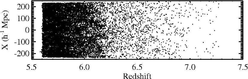
Figure 1: Redshift versus the (co-moving) $X$-coordinate for all objects within a slice of width $\Delta Y=250$ $h^{-1}$ Mpc along the $Y$-axis.

Galaxies were modeled by applying semi-analytic prescriptions of galaxy formation to the stored halo merger trees. The techniques and recipes include gas cooling, star formation, reionizaton heating, supernova feedback, black hole growth, and “radio-mode” feedback from galaxies with a static hot gas atmosphere, and are described in Croton et al. (2006). The photometric properties of galaxies are then modeled using stellar population synthesis models, including a simple dust model. Here we use the updated models ‘delucia2006a’ of De Lucia & Blaizot (2007) that have been made publicly available through an advanced database structure on the MR website (Lemson & Virgo Consortium, 2006).

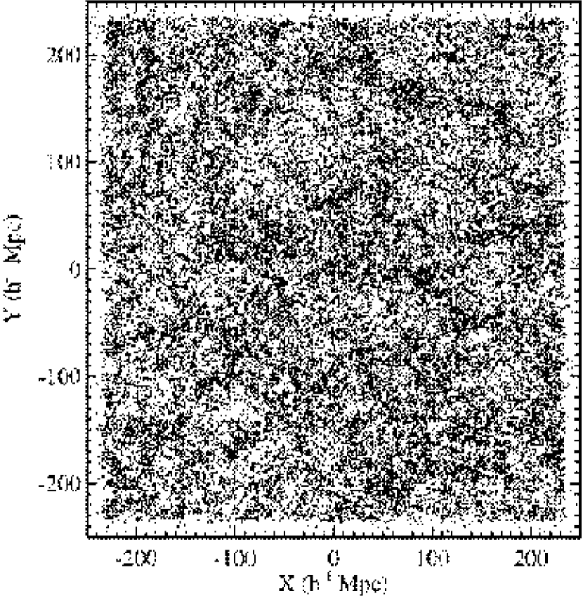
Figure 2: The simulation box showing the positions in co-moving coordinates of all objects identified as $i_{775}$-dropout galaxies to $z_{850}$$=$27.0 mag.

2.2 Construction of a large mock survey at $z\sim 6$

We used the discrete MR snapshots to create a large, continous mock survey of $i_{775}$-dropout galaxies at $z\sim 6$. The general principle of transforming a series of discrete snapshots into a mock pencil beam survey entails placing a virtual observer somewhere in the simulation box at $z=0$ and carving out all galaxies as they would be observed in a pencil beam survey along that observer’s line of sight. This technique has been described in great detail in Blaizot et al. (2005) and Kitzbichler & White (2007). In general, one starts with the snapshot $i=63$ at $z=0$ and records the positions, velocities and physical properties of all galaxies within the cone out to a comoving distance corresponding to that of the next snapshot. For the next segment of the cone, one then use the properties as recorded in snapshot $i=62$, and so on. The procedure relies on the reasonable assumption that the large-scale structure (positions and velocities of galaxies) evolves relatively slowly between snapshots. By replicating the simulation box along the lightcone and limiting the opening angle of the cone, one can in principle construct unique lightcones out to very high redshift without crossing any region in the simulation box more than once. The method is straightforward when done in comoving coordinates in a flat cosmology using simple Euclidean geometry (Kitzbichler & White, 2007).

Because the comoving distances or redshifts of galaxies recorded at a particular snapshot do not correspond exactly to their effective position along the lightcone, we need to correct their magnitudes by interpolating over redshift as follows:

$$M_{cor}[z(d)]=M(z_{i})+\frac{dM}{dz}[z(d)-z_{i})],$$ (1)

where $M_{cor}[z(d)]$ is the observer-frame absolute magnitude at the observed redshift, $z(d)$ (including peculiar velocities along the line of sight), $M(z_{i})$ is the magnitude at redshift $z_{i}$ corresponding to the $i$th snapshot, and $dM/dz$ is the first order derivative of the observer-frame absolute magnitude. The latter quantity is calculated for each galaxy by placing it at neighbouring snapshots, and ensures that the $K$-correction is taken into account (Blaizot et al., 2005). Finally, we apply the mean attenuation of the intergalactic medium using Madau (1995) and calculate the observer-frame apparent magnitudes in each filter.

In this paper, we use the fact that the selection of $z\sim 6$ galaxies through the i-dropout technique is largely free of contamination from objects at lower (and higher) redshift (Bouwens et al., 2006) provided that the observations are deep enough. Because the transverse size of the MR simulation box (500 $h^{-1}$ Mpc) corresponds to a comoving volume between $z\approx 5.6$ and $z\approx 7.3$ (the typical redshift range of $i$-dropouts surveys) we can use the three simulation snapshots centered at $z=5.7$, $z=6.2$ and $z=6.7$ to create a mock survey spanning this volume, while safely neglecting objects at other redshifts.

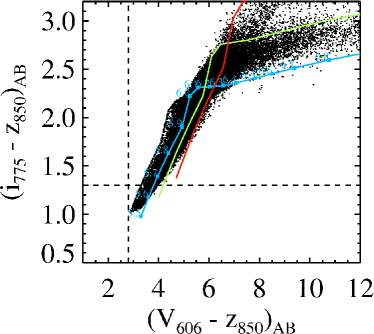
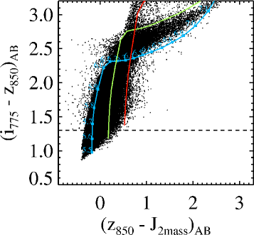
Figure 3: Colour-colour diagrams of the MR mock $i_{775}$-dropout survey. To guide the eye we have indicated tracks showing the colours of a 100 Myr old continuous starburst model from Bruzual & Charlot (2003) for different amounts of reddening in $E(B-V)$ of 0.0 (blue), 0.2 (green), and 0.4 (red). Redshifts are indicated along the zero-reddening track. Only objects at $z>5.6$ are included in the simulations, as $i_{775}$-dropouts surveys have been demonstrated to have very little contamination (see text for details).

We extracted galaxies from the MR database by selecting the $Z-$axis of the simulation box to lie along the line-of-sight of our mock field. In order to compare with the deepest current surveys, we calculated the apparent magnitudes in the HST/ACS $V_{606}$, $i_{775}$ and $z_{850}$ filters and the 2MASS $J$, $H$ and $K_{S}$ filters. We derived observed redshifts from the comoving distance along the line of sight (including the effect of peculiar velocities), applied the $K$-corrections and IGM absorption, and calculated the apparent magnitudes in each band. Fig. 1 shows the spatial $X$-coordinate versus the redshift of objects in the simulated lightcone. Fig. 2 shows the entire simulated volume projected along the $Z$- or redshift axis. These figures show that there exists significant filamentary and strongly clustered substructure at $z\approx 6$, both parallel and perpendicular to the line-of-sight.

Our final mock survey has a comoving volume of $\sim 0.3$ Gpc³, and spans an area of $4.4\degr\times 4.4\degr$ when projected onto the sky. It contains $\sim 1.6\times 10^{5}$ galaxies at $z=5.6-7.3$ with $z\leq 27.5$ mag (corresponding to an absolute magnitude of $M_{UV,AB}\simeq-19.2$ mag, about one mag below $M^{*}_{UV,z=6}$). For comparison and future reference, we list the main $i$-dropout surveys together with their areal coverage and detection limit in Table 1.

2.3 Colour-colour selection

In the left panel of Fig. 3 we show the $V_{606}-z_{850}$ vs. $i_{775}-z_{850}$ colour-colour diagram for all objects satisfying $z\leq 27.0$. The $i$-dropouts populate a region in colour-colour space that is effectively isolated from lower redshift objects using a simple colour cut of $i_{775}-z_{850}\gtrsim 1.3-1.5$. Note that although our simulated survey only contains objects at $z>5.6$, it has been shown (Stanway et al., 2003; Dickinson et al., 2004; Bouwens et al., 2004a, 2006) that this colour cut is an efficient selection criterion for isolating starburst galaxies at $z\sim 6$ with blue $z_{850}$$-J$ colours (see right panel of Fig. 3). For reference, we have overplotted colour tracks for a 100 Myr old, continuous star formation model as a function of redshift; different colour curves show results for different amounts of reddening by dust. As can be seen, these simple models span the region of colour-colour space occupied by the MR galaxies. At $z<6$, galaxies occupy a tight sequence in the plane. At $z>6$, objects fan out because the $V_{606}-z_{850}$ colour changes strongly as a function of redshift, while the $i_{775}-z_{850}$ colour is more sensitive to both age and dust reddening. Because of the possibility of intrinsically red interlopers at $z\sim 1-3$, the additional requirement of a non-detection in $V_{606}$, or a very red $V_{606}-z_{850}\gtrsim 3$ colour, if available, is often included in the selection. Because the selection based on $i_{775}-z_{850}\gtrsim 1.3$ introduces a small bias against objects having strong Ly$\alpha$ emission at $z\lesssim 6$ (Malhotra et al., 2005; Stanway et al., 2007), we have statistically included the effect of Ly$\alpha$ on our sample selection by randomly assigning Ly$\alpha$ with a rest-frame equivalent width of 30Å to 25% of the galaxies in our volume, and recalculating the $i_{775}-z_{850}$ colours. The inclusion of Ly$\alpha$ leads to a reduction in the number of objects selected of $\sim 3$% (see also Bouwens et al., 2006).

2.4 $i$-dropout number densities

In Table 2 we list the surface densities of $i_{775}$-dropouts selected in the MR mock survey as a function of limiting $z_{850}$-magnitude and field size. For comparison, we calculated the surface densities for regions having areas comparable to some of the main $i_{775}$-dropout surveys: the SDF (876 arcmin²), two GOODS fields (320 arcmin²), a single GOODS field (160 arcmin²), and a HUDF-sized field (11.2 arcmin²). The errors in Table 2 indicate the $\pm 1\sigma$ deviation measured among a large number of similarly sized fields selected from the mock survey, and can be taken as an estimate of the influence of (projected) large-scale structure on the number counts (usually referred to as “cosmic variance” or “field-to-field variations”). At faint magnitudes, the strongest observational constraints on the $i_{775}$-dropout density come from the HST surveys. Our values for a GOODS-sized survey are 105, 55 and 82% of the values given by the most recent estimates by B07 for limiting $z_{850}$ magnitudes of 27.5, 26.5 and 26.0 mag, respectively, and consistent within the expected cosmic variance allowed by our mock survey. Because the total area surveyed by B06 is about 200$\times$ smaller than our mock survey, we also compare our results to the much larger SDF from Ota et al. (2008). At $z=26.5$ mag the number densities of $\sim$0.18 arcmin^-2 derived from both the real and mock surveys are perfectly consistent.

Last, we note that in order to achieve agreement between the observed and simulated number counts at $z\sim 6$, we did not require any tweaks to either the cosmology (e.g., see Wang et al., 2008, for the effect of different WMAP cosmologies), or the dust model used (see Kitzbichler & White, 2007; Guo & White, 2008, for alternative dust models better tuned to high redshift galaxies). This issue may be further investigated in a future paper.

2.5 Redshift distribution

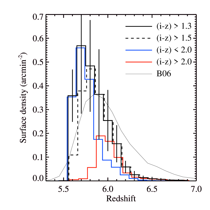
Figure 4: Redshift histograms derived from the MR mock $i$-dropout survey at the depth of $z_{850}$=27.5 mag using the selection criteria $i_{775}$–$z_{850}$$>1.3$ (thick solid line, error bars indicate the 1$\sigma$ scatter expected among GOODS-sized fields), $i_{775}$–$z_{850}$$>1.5$ (dashed line), $i_{775}$–$z_{850}$$<2.0$ (blue line), and $i_{775}$–$z_{850}$$>2.0$ (red line). The thin solid line indicates the model redshift distribution from B06 based on the HUDF.

In Fig. 4 we show the redshift distribution of the full mock survey (thick solid line), along with various subsamples selected according to different $i_{775}$–$z_{850}$ colour cuts that we will refer to later on in this paper. The standard selection of $i_{775}$–$z_{850}$$>$1.3 results in a distribution that peaks at $z\approx 5.8$. We have also indicated the expected scatter resulting from cosmic variance on the scale of GOODS-sized fields (error bars are 1$\sigma$). Some, mostly groundbased, studies make use of a more stringent cut of $i_{775}$–$z_{850}$$>1.5$ to reduce the chance of foreground interlopers (dashed histogram). Other works have used colour cuts of $i_{775}$–$z_{850}$$\lesssim 2$ (blue histogram) and $i_{775}$–$z_{850}$$\gtrsim 2$ (red histogram) in order to try to extract subsamples at $z\lesssim 6$ and $z\gtrsim 6$, respectively. As can be seen in Fig. 4, such cuts are indeed successful at broadly separating sources from the two redshift ranges, although the separation is not perfectly clean due to the mixed effects of age, dust and redshift on the $i_{775}$–$z_{850}$ colour. For reference, we have also indicated the model redshift distribution from B06 (thin solid line). This redshift distribution was derived for a much fainter sample of $z_{850}$$\lesssim$29 mag, which explains in part the discrepancy in the counts at $z\gtrsim 6.2$. Evolution across the redshift range will furthermore skew the actual redshift distribution toward lower values (see discussion in Muñoz & Loeb, 2008b). This is not included in the B06 model, and its effect is only marginally taken into account in the MR mock survey due to the relatively sparse snapshot sampling across the redshift range. Unfortunately, the exact shape of the redshift distribution is currently not very well constrained by spectroscopic samples (Malhotra et al., 2005). A more detailed analysis is beyond the scope of this paper, and we conclude by noting that the results presented below are largely independent of the exact shape of the distribution.

2.6 Physical properties of $i$-dropouts

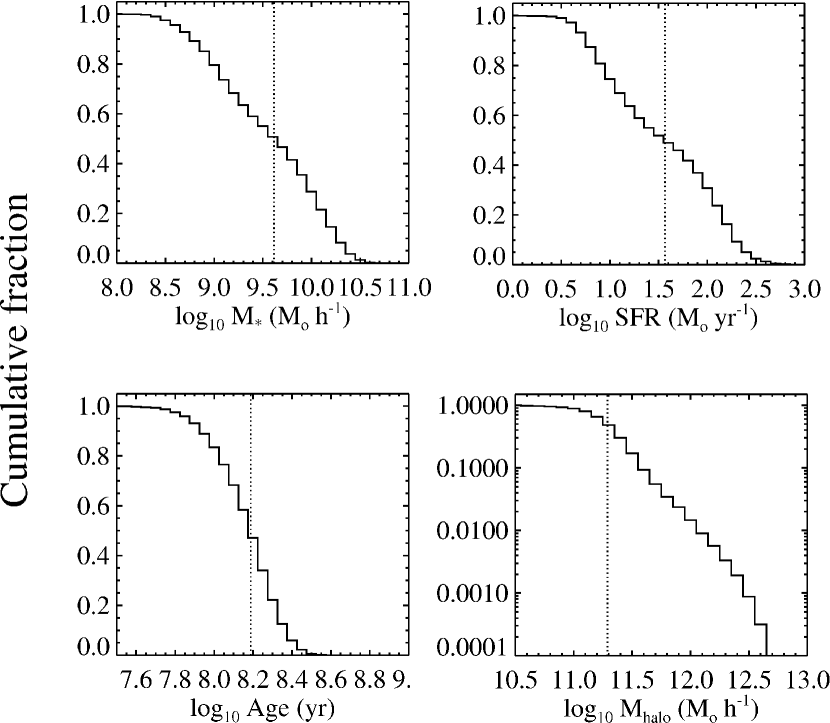
Figure 5: Physical properties of $i$-dropouts in the MR mock survey satisfying $z\leq 26.5$ mag. We plot the cumulative fractions of galaxies with stellar masses, star formation rates, stellar ages and halo masses greater than a given value. Top left: Distribution of stellar masses. The median stellar mass is $\sim 4\times 10^{9}$ $M_{\odot}$ h^-1 (dotted line). Top right: Distribution of SFRs. The median SFR is $\sim 30$ $M_{\odot}$ yr^-1 (dotted line). Bottom left: Distribution of mass-weighted ages. The median age is $\sim$160 Myr (dotted line). Bottom right: Distribution of halo masses. The median halo mass is $\sim 2\times 10^{11}$ $M_{\odot}$ h^-1 (dotted line).

Although a detailed study of the successes and failures in the semi-analytic modeling of galaxies at $z\sim 6$ is not the purpose of our investigation, we believe it will be instructive for the reader if we at least summarize the main physical properties of the model galaxies in our mock survey. Unless stated otherwise, throughout this paper we will limit our investigations to $i$-dropout samples having a limiting magnitude of $z_{850}$=26.5 mag, comparable to $M^{*}_{UV}$ at $z=6$ (see Bouwens et al., 2007). This magnitude typically corresponds to model galaxies situated in dark matter halos of at least 100 dark matter particles ($\sim 10^{11}$ M_⊙ h^-1). This ensures that the evolution of those halos and their galaxies has been traced for some time prior to the snapshot from which the galaxy was selected. In this way, we ensure that the physical quantities derived from the semi-analytic model are relatively stable against snapshot-to-snapshot fluctuations. A magnitude limit of $z_{850}$=26.5 mag also conveniently corresponds to the typical depth that can be achieved in deep groundbased surveys or relatively shallow HST-based surveys.

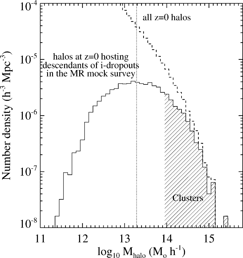
Figure 6: Number density versus halo mass of the $z=0$ dark matter halos hosting descendants of $i$-dropouts at $z\sim 6$ to a limiting depth of $z_{850}$$\leq$26.5 mag. The median $i$-dropout descendant halo mass is a few times $10^{13}$ $M_{\odot}$ (dotted line). The halo mass function of all MR halos at $z=0$ is indicated by the dashed line. The mass range occupied by the halos associated with galaxy clusters is indicated by the hatched region.

In Fig. 5 we plot the cumulative distributions of the stellar mass (top left), SFR (top right), and stellar age (bottom left) of the $i_{775}$-dropouts in the mock survey. The median stellar mass is $\sim 5\times 10^{9}$ $M_{\odot}$ h^-1, and about 30% of galaxies have a stellar mass greater than $10^{10}$ $M_{\odot}$. The median SFR and age are $\sim 30$ $M_{\odot}$ yr^-1 and $\sim$160 Myr, respectively, with extrema of $\sim 500$ $M_{\odot}$ yr^-1 and $\sim$400 Myr. These results are in general agreement with several studies based on modeling the stellar populations of limited samples of $i_{775}$-dropouts and Ly$\alpha$ emitters for which deep observations with HST and Spitzer exist. Yan et al. (2006) have analyzed a statistically robust sample and find stellar masses ranging from $\sim 1\times 10^{8}$ $M_{\odot}$ for IRAC-undetected sources to $\sim 7\times 10^{10}$ $M_{\odot}$ for the brightest 3.6$\mu$m sources, and ages ranging from $<$40 to 400 Myr (see also Dow-Hygelund et al., 2005; Eyles et al., 2007; Lai et al., 2007, for additional comparison data). We also point out that the maximum stellar mass of $\sim 7\times 10^{10}$ $M_{\odot}$ found in our mock survey (see top left panel) is comparable to the most massive $i$-dropouts found, and that “supermassive” galaxies having masses in excess of $\gtrsim 10^{11}$ $M_{\odot}$ are absent in both the simulations and observations (McLure et al., 2006). Last, in the bottom right panel we show the distribution of the masses of the halos hosting the model $i$-dropouts. The median halo mass is $\sim 3\times 10^{11}$ $M_{\odot}$. Our results are in the range of values reported by Overzier et al. (2006) and McLure et al. (2008) based on the angular correlation function of large $i_{775}$-dropout samples, but we note that halo masses are currently not very well constrained by the observations.

Figure 7: Number density versus stellar mass of the galaxies at $z=0$ that have at least one $i$-dropout progenitor at $z\sim 6$. The median descendant mass is $\sim 10^{11}$ $M_{\odot}$ (dotted line). The distribution of stellar mass of all MR $z=0$ galaxies is indicated for comparison (dashed line).

3 The relation between $i$-dropouts and (proto-)clusters

In this Section we study the relation between local overdensities in the $i$-dropout distribution at $z\sim 6$ and the sites of cluster formation. Throughout this paper, a galaxy cluster is defined as being all galaxies belonging to a bound dark matter halo having a dark matter mass of $\cal{M}$${}_{tophat}\geq 10^{14}$ h^-1 $M_{\odot}$ at $z=0$. In the MR we find 2,832 unique halos, or galaxy clusters, fulfilling this condition, 21 of which can be considered supermassive ($\cal{M}$${}_{tophat}\geq 10^{15}$ h^-1 $M_{\odot}$). Furthermore, a proto-cluster galaxy is defined as being a galaxy at $\sim 6$ that will end up in a galaxy cluster at $z=0$. Note that these are trivial definitions given the database structure of the Millennium Run simulations, in which galaxies and halos at any given redshift can be related to their progenitors and descendants at another redshift (Lemson & Virgo Consortium, 2006).

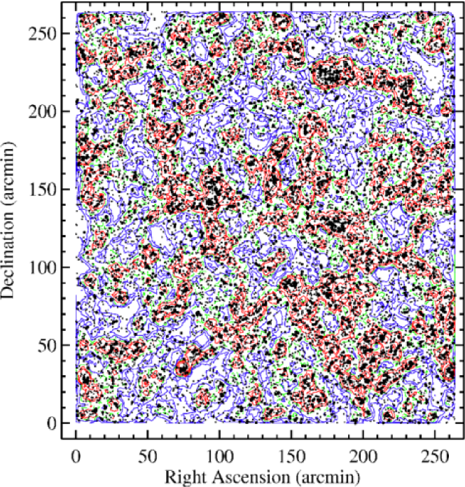
Figure 8: Projected distribution on the sky of the $z\sim 6$ $i$-dropouts selected from the MR mock survey according to the criteria $i_{775}$–$z_{850}$$>$1.3 and $z\leq 26.5$ mag (small and large points). Contours indicate regions of equal density, defined as $\delta\Sigma_{5\arcmin}\equiv(\Sigma_{5\arcmin}-\bar{\Sigma}_{5\arcmin})/\bar{\Sigma}_{5\arcmin}$, $\Sigma_{5\arcmin}$ and $\bar{\Sigma}_{5\arcmin}$ being the local and mean surface density measured in circular cells of 5′ radius. Over- and underdense regions of $\delta\Sigma_{5\arcmin}=\pm[0.25,0.5,1.0]$ are shown in red and blue contours, respectively. The mean density ($\delta\Sigma_{5\arcmin}=0$) is indicated by the green dashed contour. Large black points mark proto-cluster galaxies that end up in galaxy clusters at $z=0$.

3.1 Properties of the $z=0$ descendants of $i$-dropouts

In Fig. 6 we plot the distribution of number densities of the central halos that host the $z=0$ descendants of the $i$-dropouts in our mock survey as a function of the halo mass. The median halo mass hosting the $i$-dropout descendants at $z=0$ is $3\times 10^{13}$ $M_{\odot}$ h^-1 (dotted line). For comparison we indicate the mass distribution of all halos at $z=0$ (dashed line). The plot shows that the fraction of halos that can be traced back to a halo hosting an $i$-dropout at $z\sim 6$ is a strong function of the halo mass at $z=0$. 45% of all cluster-sized halos at $z=0$ (indicated by the hatched region) are related to the descendants of halos hosting $i$-dropouts in our mock survey, and 77% of all clusters at $z=0$ having a mass of $\cal{M}$$>7\times 10^{14}$ $M_{\odot}$ h^-1 can be traced back to at least one progenitor halo at $z\sim 6$ hosting an $i$-dropout. This implies that the first seeds of galaxy clusters are already present at $z\sim 6$. In addition, many $i$-dropout galaxies and their halos may merge and end up in the same descendant structures at $z=0$, which was not accounted for in our calculation above where we only counted unique halos at $z=0$. In fact, about $\sim$34% ($\sim$2%) of all $i$-dropouts ($z_{850}$$\leq$26.5) in the mock survey will end up in clusters of mass $>1\times 10^{14}$ ($>7\times 10^{14}$) $M_{\odot}$ h^-1 at $z=0$. This implies that roughly one third of all galaxies one observes in a typical $i$-dropout survey can be considered “proto-cluster” galaxies. The plot further shows that the majority of halos hosting $i$-dropouts at $z\sim 6$ will evolve into halos that are more typical of the group environment. This is similar to the situation found for Lyman break or dropout galaxies at lower redshifts (Ouchi et al., 2004).

In Fig. 7 we plot the stellar mass distribution of those $z=0$ galaxies that host the descendants of the $i$-dropouts. The present-day descendants are found in galaxies having a wide range of stellar masses ($\cal{M}$${}_{*}\simeq 10^{9-12}$ $M_{\odot}$), but the distribution is skewed towards the most massive galaxies in the MR simulations. The median stellar mass of the descendants is $\sim 10^{11}$ $M_{\odot}$ (dotted line in Fig. 7).

3.2 Detecting proto-clusters at $z\sim 6$

We will now focus on to what extent local overdensities in the $i$-dropout distribution at $z\approx 6$ may trace the progenitor seeds of the richest clusters of galaxies in the present-day Universe. In Fig. 8 we plot the sky distribution of the $i$-dropouts in our $4.4\degr\times 4.4\degr$ MR mock survey (large and small circles). Large circles indicate those $i$-dropouts identified as proto-cluster galaxies. We have plotted contours of $i$-dropout surface density, $\delta_{\Sigma,5^{\prime}}\equiv(\Sigma_{5^{\prime}}-\bar{\Sigma}_{5^{\prime}})/\bar{\Sigma}_{5^{\prime}}$, $\Sigma_{5\arcmin}$ and $\bar{\Sigma}_{5\arcmin}$ being the local and mean surface density measured in circular cells of 5′ radius. Negative contours representing underdense regions are indicated by blue lines, while positive contours representing overdense regions are indicated by red lines. The green dashed lines indicate the mean density. The distribution of proto-cluster galaxies (large circles) correlates strongly with positive enhancements in the local $i$-dropout density distribution, indicating that these are the sites of formation of some of the first clusters. In Fig. 9 we plot the frequency distribution of the $i$-dropouts shown in Fig. 8, based on a counts-in-cells analysis of 20,000 randomly placed ACS-sized fields of $3.4\arcmin\times 3.4\arcmin$ (solid histograms). On average, one expects to find about 2 $i$-dropouts in a random ACS pointing down to a depth of $z_{850}$$=$26.5, but the distribution is skewed with respect to a pure Poissonian distribution as expected due to the effects of gravitational clustering. The Poissonian expectation for a mean of 2 $i$-dropouts is indicated by a thin line for comparison. The panel on the right shows a zoomed-in view to give a better sense of the small fraction of pointings having large numbers of $i$-dropouts. Also in Fig. 9 we have indicated the counts histogram derived from a similar analysis performed on $i$-dropouts extracted from the GOODS survey using the samples of B06. The GOODS result is indicated by the dotted histogram, showing that it lies much closer to the Poisson expectation than the MR mock survey. This is of course expected as our mock survey covers an area over 200$\times$ larger than GOODS and includes a much wider range of environments. To illustrate that the (small) fraction of pointings with the largest number of objects is largely due to the presence of regions associated with proto-clusters, we effectively “disrupt” all protoclusters by randomizing the positions of all protocluster galaxies and repeat the counts-in-cells calculation. The result is shown by the dashed histograms in Fig. 9. The excess counts have largely disappeared, indicating that they were indeed due to the proto-clusters. The counts still show a small excess over the Poissonian distribution due to the overall angular clustering of the $i$-dropout population.

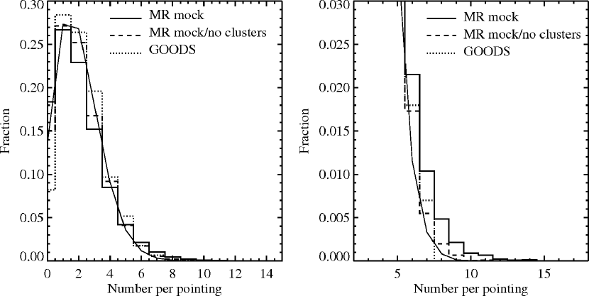
Figure 9: Counts-in-cells frequency distribution of the $i$-dropouts shown in Fig. 8, based on 20,000 randomly placed ACS-sized fields of $3.4\arcmin\times 3.4\arcmin$. The panel on the right shows a zoomed-in view to give a better sense of the small fraction of pointings having large numbers of $i$-dropouts. In both panels, the thick solid line indicates the frequency distribution of the full MR mock survey. The dashed line indicates how the distribution changes if we “disrupt” all protocluster regions of Fig. 8 by randomizing the positions of the galaxies marked as proto-cluster galaxy. The dotted line indicates the frequency distribution of a large sample of $i$-dropouts selected from the GOODS survey by B06 using identical selection criteria. Thin solid lines indicate the Poisson distribution for a mean of 2 $i$-dropouts per pointing.

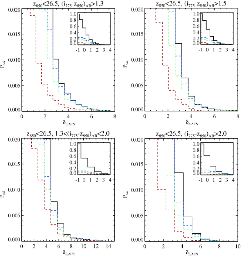
Figure 10: Panels show the cumulative probability distributions of finding regions having a surface overdensity $>\delta_{\Sigma,ACS}$ of $i$-dropouts for the four samples extracted from the MR mock survey based on colour cuts of $i_{775}$–$z_{850}$$>1.3$ (top-left), $i_{775}$–$z_{850}$$>1.5$ (top-right), $1.3<$$i_{775}$–$z_{850}$$<2.0$ (bottom-left), and $i_{775}$–$z_{850}$$>2.0$ (bottom-right). The inset plots show the full probability distributions. Dashed, coloured lines indicate the joint probability of finding cells having an overdensity $>\delta_{\Sigma,ACS}$ and those cells consisting of at least 25% (blue), 50% (green) and 75% proto-cluster galaxies.

We can use our counts-in-cells analysis to predict the cumulative probability, $P_{>\delta}$, of randomly finding an $i$-dropout overdensity equal or larger than $\delta_{\Sigma,ACS}$. The resuls are shown in Fig. 10. The four panels correspond to the subsamples defined using the four different $i_{775}$–$z_{850}$ colour cuts (see §2.5 and Fig. 4). Panel insets show the full probability range for reference. The figure shows that the probability of finding, for example, cells having a surface overdensity of $i$-dropouts of $\gtrsim$3 is about half a percent for the $i_{775}$–$z_{850}$$>$1.3 samples (top left panel, solid line). The other panels show the dependence of $P_{>\delta}$ on $i$-dropout samples selected using different colour cuts. As the relative contribution from for- and background galaxies changes, the density contrast between real, physical overdensities on small scales and the “field” is increased.

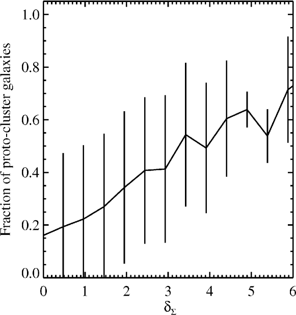
Figure 11: The average fraction of $i$-dropouts marked as proto-cluster galaxies contained in ACS-sized cells as a function of cell overdensity. Error bars are $1\sigma$. There is a clear trend showing that larger surface overdensities are associated with a larger contribution from galaxies in proto-clusters, albeit with significant scatter.

The results presented in Fig. 10 provide us with a powerful way to interpret many observational findings. Specifically, overdensities of $i$-dropouts have been interpreted as evidence for large-scale structure associated with proto-clusters, at least qualitatively. Although Fig. 10 tells us the likelihood of finding a given overdensity, this is not sufficient by itself to answer the question whether that overdensity is related to a proto-cluster due to a combination of several effects. First, because we are mainly working with photometrically selected samples consisting of galaxies spanning about one unit redshift, projection effects are bound to give rise to a range of surface densities. Second, the number counts may show significant variations as a function of position and environment resulting from the large-scale structure. The uncertainties in the cosmic variance can be reduced by observing fields that are larger than the typical scale length of the large-scale structures, but this is often not achieved in typical observations at $z\sim 6$. Third, surface overdensities that are related to genuine overdensities in physical coordinates are not necessarily due to proto-clusters, as we have shown that the descendents of $i$-dropouts can be found in a wide range of environments at $z=0$, galaxy groups being the most common (see Fig. 6). We have separated the contribution of these effects to $P_{>\delta}$ from that due to proto-clusters by calculating the fraction of actual proto-cluster $i$-dropouts in each cell of given overdensity $\delta$. The results are also shown in Fig. 10, where dashed histograms indicate the combined probability of finding a cell of overdensity $\geq\delta$ consisting of more than 25 (blue lines), 50 (green lines) and 75% (red lines) protocluster galaxies. The results show that while, for example, the chance of $P(\delta\geq 2.5)$ is about 1%, the chance that at least 50% of the galaxies in such cells are proto-cluster galaxies is only half that, about 0.5% (see top left panel in Fig. 10). The figure goes on to show that the fractions of protocluster galaxies increases significantly as the overdensity increases, indicating that the largest (and rarest) overdensities in the $i$-dropout distribution are related to the richest proto-cluster regions. This is further illustrated in Fig. 11 in which we plot the average and scatter of the fraction of proto-cluster galaxies as a function of $\delta$. Although the fraction rises as the overdensity increases, there is a very large scatter. At $\delta\approx 4$ the average fraction of protocluster galaxies is about 0.5, but varies significantly between 0.25 and 0.75 (1$\sigma$).

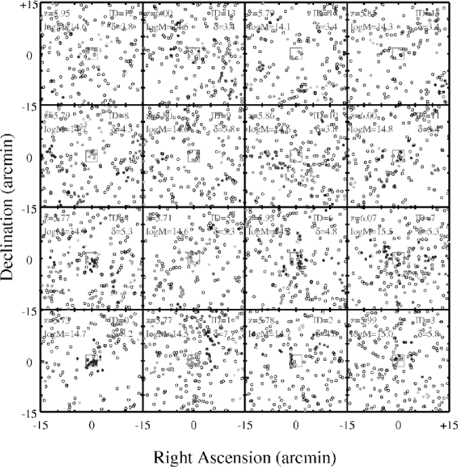
Figure 12: Panels show the angular distribution of $i_{775}$-dropouts in 30′$\times$30′ areas centered on each of 16 protoclusters associated with overdensities $\delta_{\Sigma,ACS}\gtrsim 3$. Field galaxies are drawn as open circles, and cluster galaxies as filled circles that are colour coded according to their cluster membership. The ACS field-of-view is indicated by a red square. Numbers near the top of each panel indicate the ID, redshift, overdensity and cluster mass (at $z=0$) of the protoclusters in the center of each panel.

It will be virtually impossible to estimate an accurate cluster mass at $z=0$ from a measured surface overdensity at $z\sim 6$. Although there is a correlation between cluster mass at $z=0$ and $i$-dropout overdensity at $z\sim 6$, the scatter is significant. Many of the most massive ($\cal{M}$$>$$10^{15}$ $M_{\odot}$) clusters have very small associated overdensities, while the progenitors of fairly low mass clusters ($\cal{M}$$\sim$$10^{14}$ $M_{\odot}$) can be found associated with regions of relatively large overdensities. However, the largest overdensities are consistently associated with the progenitors of $\cal{M}$$\sim 5\times 10^{14}-1\times 10^{15}$ $M_{\odot}$ clusters.

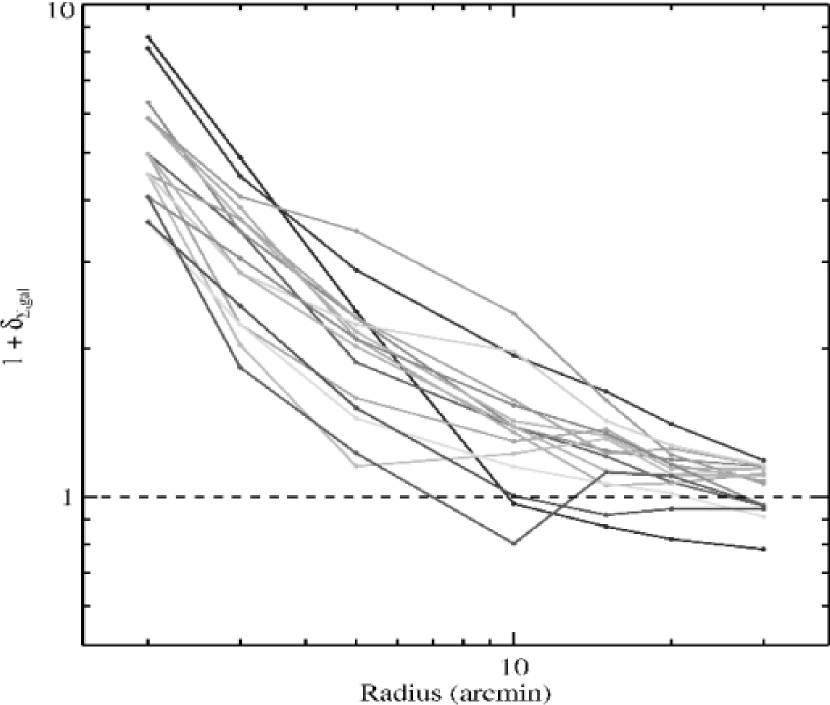
Figure 13: Lines show overdensity as a function of radius for each of the protocluster regions shown in Fig. 12.

3.3 Some examples

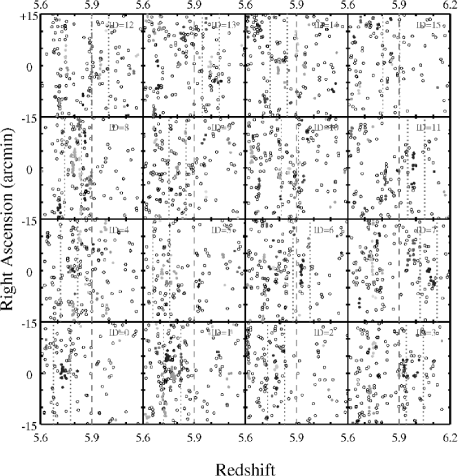
Figure 14: Panels show redshift versus one of the angular coordinates of $i_{775}$-dropouts for each of the protocluster regions shown in Fig. 12. Field galaxies are drawn as open circles, and cluster galaxies as filled circles that are colour coded according to their cluster membership as in Fig. 12. Red dashed lines mark $z=5.9$, which roughly corresponds to, respectively, the upper and lower redshift of samples selected by placing a cut at $i_{775}$–$z_{850}$$\lesssim$2 and $i_{775}$–$z_{850}$$\gtrsim$2. Blue dotted lines mark the redshift range ($\Delta z\approx 0.1$) probed by narrowband Ly$\alpha$ filters.

Although the above sections yield useful statistical results, it is interesting to look at the detailed angular and redshift distributions of the $i_{775}$-dropouts in a few of the overdense regions. In Fig. 12 we show 16 30′$\times$30′ regions having overdensities ranging from $\delta_{\Sigma,ACS}\sim 8$ (bottom left panel) to $\sim 3$ (top right panel). In each panel we indicate the relative size of an ACS pointing (red square), and the redshift, overdensity and present-day mass of the most massive protoclusters are given in the top left and right corners. Field galaxies are drawn as open circles, while protocluster galaxies are drawn as filled circles. Galaxies belonging to the same proto-cluster are drawn in the same colour. While some regions contain relatively compact protoclusters with numerous members inside the 3.4′$\times$3.4′ ACS field-of-view (e.g. panels #0, 1 and 8), other regions may contain very few or highly dispersed galaxies. Also, many regions contain several overlapping protoclusters as the selection function is sensitive to structures from a relatively wide range in redshift inside the 30′$\times$30′ regions plotted. Although the angular separation between galaxies belonging to the same protocluster is typically smaller than $\sim$10′ or 25 Mpc (comoving), Fig. 13 shows that the overdensities of regions centered on the protoclusters are significantly positive out to much larger radii of between 10 to 30′, indicating that the protoclusters form inside very large filaments of up to 100 Mpc in size that contribute significantly to the overall (field) number counts in the protocluster regions. In Fig. 14 we plot the redshift coordinate against one of the angular coordinates using the same regions and colour codings as in Fig. 12. Protoclusters are significantly more clumped in redshift space compared to field galaxies, due to flattening of the velocity field associated with the collapse of large structures. In each panel, a red dashed line marks $z=5.9$, which roughly corresponds to, respectively, the upper and lower redshift of samples selected by placing a cut at $i_{775}$–$z_{850}$$\lesssim$2 and $i_{775}$–$z_{850}$$\gtrsim$2 (see the redshift selection functions in Fig. 4). Such colour cuts may help reduce the contribution from field galaxies by about 50%, depending on the redshift one is interested in. We also mark the typical redshift range of $\Delta z\approx 0.1$ probed by narrowband filters centered on the redshift of each protocluster using blue dotted lines. As we will show in more detail in §4.2 below, such narrowband selections offer one of the most promising methods for finding and studying the earliest collapsing structures at high redshift, because of the significant increase in contrast between cluster and field regions. However, such surveys are time-consuming and only probe the part of the galaxy population that is bright in the Ly$\alpha$ line.

4 Comparison with observations from the literature

Our mock survey of $i$-dropouts constructed from the MR, due to its large effective volume, spans a wide range of environments and is therefore ideal for making detailed comparisons with observational studies of the large-scale structure at $z\sim 6$. In the following subsections, we will make such comparisons with two studies of candidate proto-clusters of $i$-dropouts and Ly$\alpha$ emitters found in the SDF and SXDF.

4.1 The candidate proto-cluster of Ota et al. (2008)

When analysing the sky distribution of $i$-dropouts in the 876 arcmin² Subaru Deep Field, Ota et al. (2008) (henceforward O08) discovered a large surface overdensity, presumed to be a proto-cluster at $z\sim 6$. The magnitude of the overdensity was quantified as the excess of $i$-dropouts in a circle of 20 Mpc comoving radius. The region had $\delta_{\Sigma,20\mathrm{Mpc}}=0.63$ with $3\sigma$ significance. Furthermore, this region also contained the highest density contrast measured in a 8 Mpc comoving radius $\delta_{\Sigma,8\mathrm{Mpc}}=3.6$ ($5\sigma$) compared to other regions of the SDF. By relating the total overdensity in dark matter to the measured overdensity in galaxies through an estimate of the galaxy bias parameter, the authors estimated a mass for the proto-cluster region of $\sim 1\times 10^{15}$ $M_{\odot}$.

We use our mock survey to select $i$-dropouts with $i_{775}$–$z_{850}$$>1.5$ and $z_{850}$$<26.5$, similar to O08. The resulting surface density was 0.16 arcmin^-2 in very good agreement with the value of 0.18 arcmin^-2 found by O08. In Fig. 15 we plot the sky distribution of our sample, and connect regions of constant (positive) density $\delta_{\Sigma,20\mathrm{Mpc}}$. Next we selected all regions that had $\delta_{\Sigma,20\mathrm{Mpc}}\geq 0.63$. These regions are indicated by the large red circles in Fig. 15. We find $\sim$30 (non-overlapping) regions in our entire mock survey having $\delta_{\Sigma,20\mathrm{Mpc}}=0.6-2.0$ at $2-7\sigma$ significance, relative to the mean dropout density of $\bar{\Sigma}_{20\mathrm{Mpc}}\approx 32$. Analogous to Fig. 8, we have marked all $i$-dropouts associated with proto-clusters with large symbols. It can be seen clearly that the proto-cluster galaxies are found almost exclusively inside the regions of enhanced local surface density indicated by the contour lines, while the large void regions are virtually depleted of proto-cluster galaxies. Although the 30 regions of highest overdensity selected to be similar to the region found by O08 coincide with the highest peaks in the global density distribution across the field, it is interesting to point out that in some cases the regions contain very few actual proto-cluster galaxies, e.g., the regions at (RA,DEC)=(10,150) and (80,220) in Fig. 15. We therefore introduce a proto-cluster “purity” parameter, $\cal{R}_{\mathrm{pc}}$, defined as the ratio of galaxies in a (projected) region that belong to protoclusters to the total number of galaxies in that region. We find $\cal{R}_{\mathrm{pc,20Mpc}}\approx$16–50%. The purest or richest proto-clusters are found in regions having a wide range in overdensities, e.g., the region at (175,225) with $\delta_{\Sigma,20\mathrm{Mpc}}=2.2$, $\cal{R}_{\mathrm{pc,20Mpc}}=$50%), and the region at (200,40) with $\delta_{\Sigma,20\mathrm{Mpc}}=0.9$, $\cal{R}_{\mathrm{pc,20Mpc}}=$40%. Following O08 we also calculate the maximum overdensity in each region using cells of 8 Mpc radius. We find $\delta_{\Sigma,8\mathrm{Mpc}}=1.1-3.5$ with $2-6\sigma$ significance. These sub-regions are indicated in Fig. 15 using smaller circles. Interestingly, there is a very wide range in proto-cluster purity of $\cal{R}_{\mathrm{pc,8Mpc}}\approx$0–80%. The largest overdensity in Fig. 15 at (175,225) corresponds to the region giving birth to the most massive cluster. By $z=0$, this region has grown into a “supercluster” region containing numerous clusters, two of which have $M>10^{15}$ $M_{\odot}$.

We conclude that local overdensities in the distribution of $i$-dropouts on scales of $\sim$10-50 comoving Mpc similar to the one found by O08 indeed trace the seeds of massive clusters. Because our mock survey is about 80$\times$ larger than the SDF, we expect that one would encounter such proto-cluster regions in about one in three (2.7) SDF-sized fields on average. However, the fraction of actual proto-cluster galaxies is in the range 16–50% (0–80% for 8 Mpc radius regions). This implies that while one can indeed find the overdense regions where clusters are likely to form, there is no way of verifying which galaxies are part of the proto-cluster and which are not, at least not when using photometrically selected samples. These results are consistent with our earlier finding that there is a large scatter in the relation between the measured surface overdensity and both cluster “purity” and the mass of its descendant cluster at $z=0$ (Sect. 3.2).

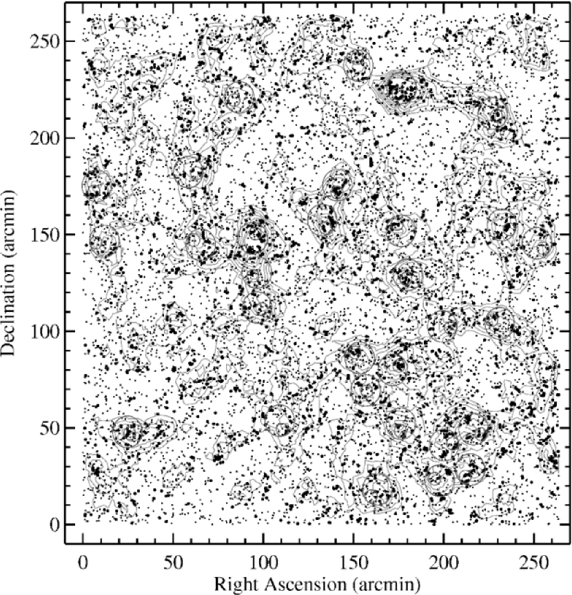
Figure 15: The sky distribution of $i$-dropouts selected using criteria matched to those of Ota et al. (2008). Grey solid lines are surface density contours of $\delta_{\Sigma,20\mathrm{Mpc}}=0,+0.2,+0.4,+0.6,+0.8$ and $+1.0$. Large red dashed circles mark overdense regions of $\delta_{\Sigma,20\mathrm{Mpc}}>0.63$, corresponding to similar overdensities as that associated with the candidate $z\sim 6$ proto-cluster region found by Ota et al. (2008) in the Subaru Deep Field. Small red circles inside each region mark a subregion having the largest overdensity $\delta_{\Sigma,8\mathrm{Mpc}}$ measured in a 8 Mpc co-moving radius (projected) cell (see text for further details).

4.2 The Ly$\alpha$-selected proto-cluster of Ouchi et al. (2005)

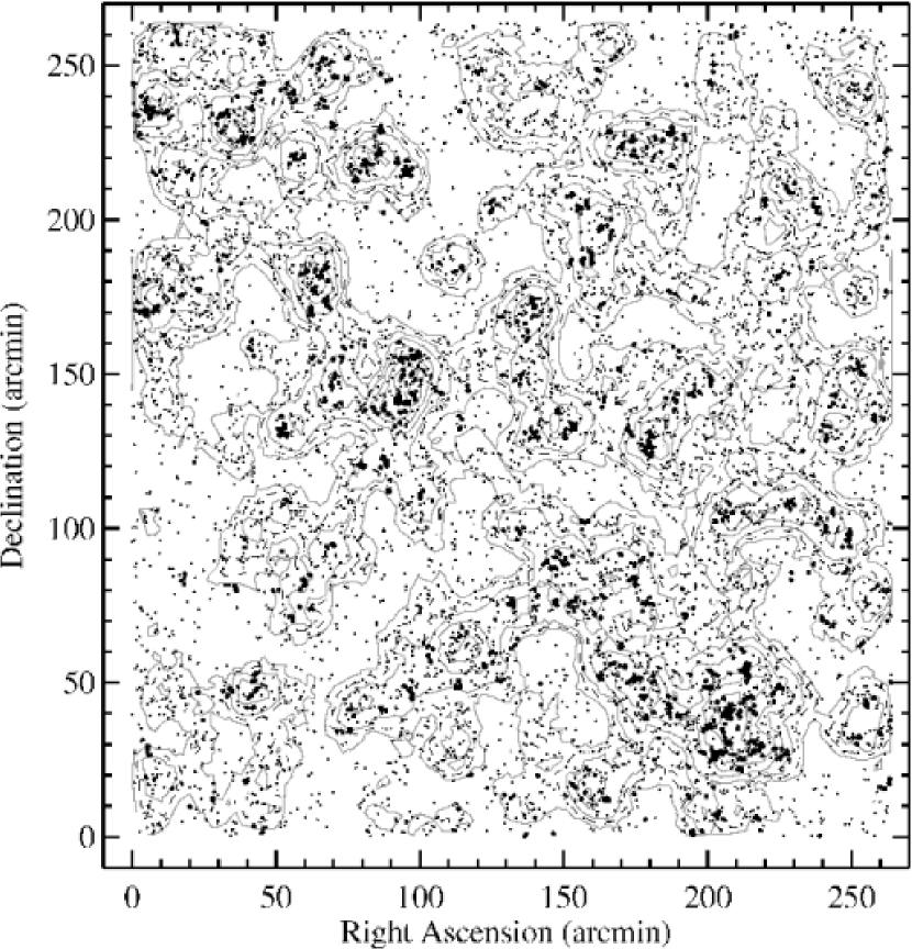
Figure 16: Mock Ly$\alpha$ survey at $\simeq 5.8\pm 0.05$ constructed from the MR mock $i_{775}$-dropout sample. Grey solid lines are surface density contours of $\delta_{\Sigma,20\mathrm{Mpc}}=-0.25$ to 3.25 with a step increase of 0.5 as in Fig. 2 of Ouchi et al. (2005). The black dashed line marks the average field density. Small circles indicate field galaxies. Large circles indicate protocluster galaxies.

The addition of velocity information gives studies of Ly$\alpha$ samples a powerful edge over purely photometrically selected $i_{775}$-dropout samples. As explained by Monaco et al. (2005, and references therein), peculiar velocity fields are influenced by the large-scale structure: streaming motions can shift the overall distribution in redshift, while the dispersion can both increase and decrease as a result of velocity gradients. Galaxies located in different structures that are not physically bound will have higher velocity dispersions, while galaxies that are in the process of falling together to form non-linear structures such as a filaments, sheets (or “pancakes”) and proto-clusters will have lower velocity dispersions.

Using deep narrow-band imaging observations of the SXDF, Ouchi et al. (2005) (O05) were able to select Ly$\alpha$ candidate galaxies at $z\simeq 5.7\pm 0.05$. Follow-up spectroscopy of the candidates in one region that was found to be significantly overdense ($\delta\gtrsim 3$) on a scale of 8 Mpc (comoving) radius resulted in the discovery of two groups (’A’ and ’B’) of Ly$\alpha$ emitting galaxies each having a very narrow velocity dispersion of $\lesssim 200$ km s^-1. The three-dimensional density contrast is on the order of $\sim 100$, comparable to that of present-day clusters, and the space density of such proto-cluster regions is roughly consistent with that of massive clusters (see O05).

In order to study the velocity fields of collapsing structures and carry out a direct comparison with O05, we construct a simple Ly$\alpha$ survey from our mock sample as follows. First, we construct a (Gaussian) redshift selection function centred on $z=5.8$ with a standard deviation of 0.04. As it is not known what causes some galaxies to be bright in Ly$\alpha$ and others not, our simulations do not include a physical prescription for Ly$\alpha$ as such. However, empirical results suggest that Ly$\alpha$ emitters are mostly young, relatively dust-free objects and a subset of the $i_{775}$-dropout population. The fraction of galaxies with high equivalent width Ly$\alpha$ is about 40%, and this fraction is found to be roughly constant as a function of the rest-frame UV continuum magnitude. Therefore, we scale our selection function so that it has a peak selection efficiency of 40%. Next, we apply this selection function to the $i_{775}$-dropouts from the mock survey to create a sample with a redshift distribution similar to that expected from a narrowband Ly$\alpha$ survey. Finally, we tune the limiting $z_{850}$ magnitude until we find a number density that is similar to that reported by O05. By setting $z_{850}$$<$26.9 mag we get the desired number density of $\sim$0.1 arcmin^-2. The mock Ly$\alpha$ field is shown in Fig. 16.

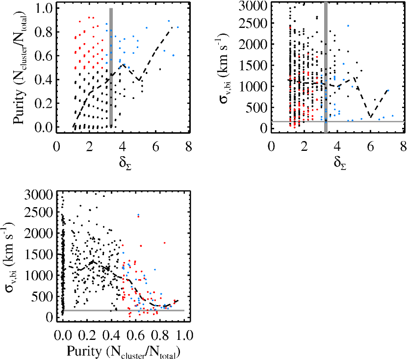
Figure 17: The correlations between surface overdensity, cluster purity and velocity dispersion for Ly$\alpha$ galaxies selected from the mock Ly$\alpha$ survey shown in Fig. 16 using randomly drawn cells of 8 Mpc (comoving) radius. Dashed lines indicate the median trends. Red points highlight regions of purity $\cal{R}>$0.5. Blue points highlight regions of $\cal{R}>$0.5 and $\delta_{\Sigma}>3$. Shaded areas mark the values obtained by Ouchi et al. (2005) for a protocluster of Ly$\alpha$ galaxies in the SDF. See text for details.

In the top left panel of Fig. 17 we plot the overdensities measured in randomly drawn regions of 8 Mpc (comoving) radius against the protocluster purity parameter, analogous to Fig. 11. Although the median purity of a sample increases with overdensity (dashed line), the scatter indicated by the points is very large even for overdensities as large as $\delta\approx 3$ found by O05 (marked by the shaded region in the top panel of Fig. 17). To guide the eye, we have plotted regions of purity $>$0.5 as red points, and regions having purity $>$0.5 and $\delta>3$ as blue points in all panels of Fig. 17. Next, we calculate the velocity dispersion, $\sigma_{v,bi}$, from the peculiar velocities of the galaxies in each region using the bi-weight estimator of Beers et al. (1990) that is robust for relatively small numbers of objects ($N\simeq 10-50$), and plot the result against $\delta$ and cluster purity in the top right and bottom left panels of Fig. 17, respectively.

Although gravitational clumping of galaxies in redshift space causes the velocity dispersions to be considerably lower than the velocity width allowed by the bandpass of the narrowband filter ($\langle\sigma_{v,bi}\rangle\simeq 1000$ km $s^{-1}$ compared to $\sigma_{NB}\approx 1800$ km $s^{-1}$ for $\sigma_{NB,z}=0.04$), the velocity dispersion is not a decreasing function of the overdensity (at least not up to $\delta\approx 3-4$) and the scatter is significant. This can be explained by the fact that proto-clusters regions are rare, and even regions that are relatively overdense in angular space still contain many galaxies that are not contained within a single bound structure. A much stronger correlation is found between dispersion and cluster purity (see bottom left panel of Fig. 17). Although the scatter in dispersion is large for regions with a purity of $\lesssim 0.5$, the smallest dispersions are associated with some of the richest protocluster regions. This can be understood because the “purest” structures represent the bound inner cores of future clusters at $z=0$. The velocity dispersions are low because these systems do not contain many field galaxies that act to inflate the velocity dispersion measurements. Therefore, the velocity dispersion correlates much more strongly with the protocluster purity than with the surface overdensity. The overdensity parameter helps, however, in reducing some of the ambiguity in the cluster richness at small dispersions (compare black and blue points at small $\sigma_{v,bi}$ in the bottom left panel). The shaded regions in Fig. 17 indicate the range of measurements of O05, implying that their structure has the characteristics of Ly$\alpha$ galaxies falling into a protocluster at $z\sim 6$.

5 Where is the large-scale structure associated with $z\sim 6$ QSOs?

For reasons explained in the Introduction, it is generally assumed that the luminous QSOs at $z\sim 6$ inhabit the most massive dark matter in the early Universe. The HST/ACS, with its deep and wide-field imaging capabilities in the $i_{775}$ and $z_{850}$ bands, has made it possible to test one possible implication of this by searching for small neighbouring galaxies tracing these massive halos. In this Section, we will first investigate what new constraint we can put on the masses of the host halos based on the observed neighbour statistics. Muñoz & Loeb (2008a) have addressed the same problem based on the excursion set formalism. Our analysis is based on semi-analytic models incorporated in the MR simulation, which we believe is likely to provide a more realistic description of galaxy properties at $z\sim 6$. We will use the simulations to evaluate what we can say about the most likely environment of the QSOs and whether they are associated with proto-clusters. We finish the Section by presenting some clear examples from the simulations that would signal a massive overdensity in future observations.

Several searches for companion galaxies in the vicinity of $z\sim 6$ QSOs have been carried out to date. In Table 1 we list the main surveys, covering in total 6 QSOs spanning the redshift range $5.8<z<6.4$. We have used the results given in Stiavelli et al. (2005), Zheng et al. (2006) and Kim et al. (2008) to calculate the surface overdensities associated with each of the QSO fields listed in Table 1. Only two QSOs were found to be associated with positive overdensities to a limiting magnitude of $z_{850}$$=$26.5: J0836+0054 ($z=5.82$) and J1030+0524 ($z=6.28$) both had $\delta_{\Sigma,\mathrm{ACS}}\approx 1$, although evidence suggests that the overdensity could be as high as $\approx 2-3$ when taking into account subclustering within the ACS field or sources selected using different $S/N$ or colour cuts (see Stiavelli et al., 2005; Zheng et al., 2006; Ajiki et al., 2006; Kim et al., 2008, for details). The remaining four QSO fields (J1306+0356 at $z=5.99$, J1630+4012 at $z=6.05$, J1048+4637 at $z=6.23$, and J1148+5251 at $z=6.43$) were all consistent with having no excess counts with $\delta_{\Sigma,\mathrm{ACS}}$ spanning the range from about $-$1 to $+$0.5 relatively independent of the method of selection (Kim et al., 2008). Focusing on the two overdense QSO fields, Fig. 10 tells us that overdensities of $\delta_{\Sigma,\mathrm{ACS}}\gtrsim 1$ are fairly common, occurring at a rate of about 17% in our $4\degr\times 4\degr$ simulation. The probability of finding a random field with $\delta_{\Sigma}\gtrsim 2-3$ is about 5 to 1%. It is evident that none of the six quasar fields have highly significant overdensities. The case for overdensities near the QSOs would strengthen if all fields showed a systematically higher, even if moderate, surface density. However, when considering the sample as a whole the surface densities of $i$-dropouts near $z\sim 6$ QSOs are fairly average, given that four of the QSO fields have lower or similar number counts compared to the field. With the exception perhaps of the field towards the highest redshift QSO J1148+5251, which lies at a redshift where the $i$-dropout selection is particularly inefficient (see Fig. 4), the lack of evidence for substantial (surface) overdensities in the QSO fields is puzzling.

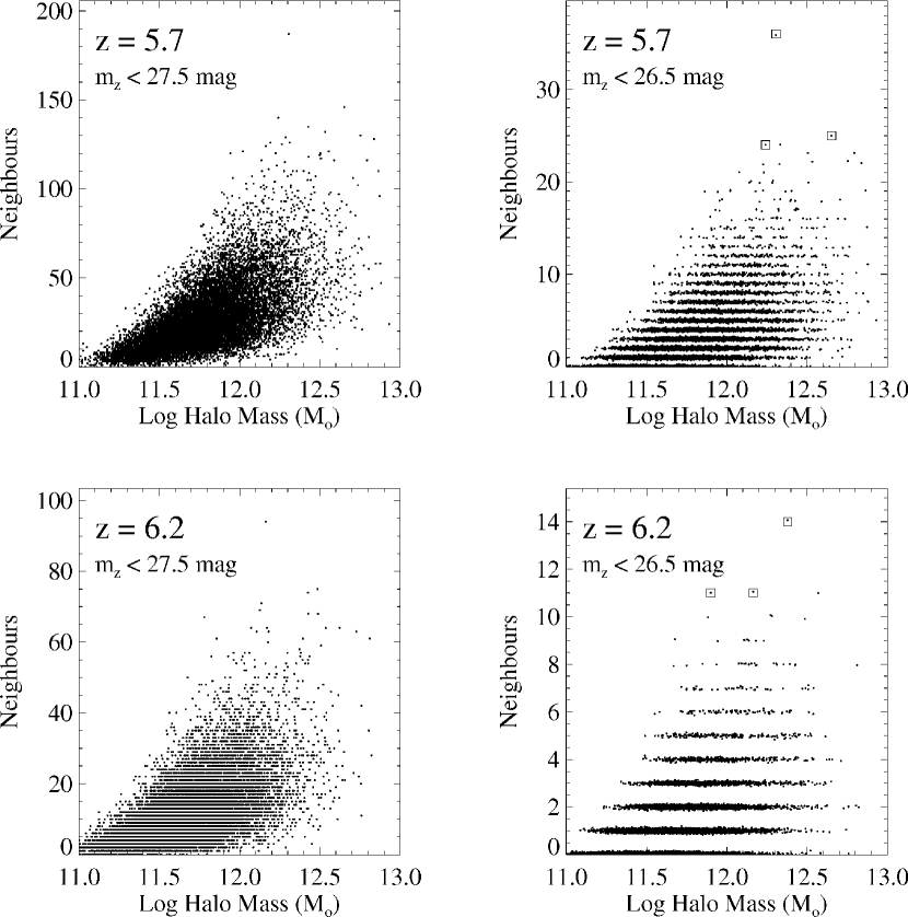
Figure 18: Panels show the number of neighbours ($i_{775}$-dropouts) in cubic regions of $(20~{}h^{-1})^{3}$ Mpc³ versus the mass of the most massive halo found in each of those regions. Top and bottom panels are for snapshots at $z=5.7$ and $z=6.2$, respectively. Left and right panels are for neighbour counts down to limiting magnitudes of $z_{850}$=27.5 (left) and $z_{850}$$=26.5$ mag, respectively. There is a wide dispersion in the number of neighbours, even for the most massive halos at $z\sim 6$. The highest numbers of neighbours are exclusively associated with the massive end of the halo mass function, allowing one to derive a lower limit for the mass of the most massive halo for a given number of neighbour counts. The scatter in the number of neighbours versus the mass of the most massive halo reduces signficantly when going to fainter magnitudes. The small squares in the panels on the right correspond to the three richest regions (in terms of $z_{850}$$<$26.5 mag dropouts) that are shown in close-up in Fig. 19.

In Fig. 18 we have plotted the number of $i_{775}$-dropouts encountered in cubic regions of $20\times 20\times 20$ $h^{-1}$ Mpc against the mass of the most massive dark matter halo found in each region. Panels on the left and on the right are for limiting magnitudes of $z_{850}$=27.5 and 26.5 mag, respectively. Because the most massive halos are so rare, here we have used the full MR snapshots at $z=5.7$ (top panels) and $z=6.2$ (bottom panels) rather than the lightcone in order to improve the statistics. There is a systematic increase in the number of neighbours with increasing maximum halo mass. However, the scatter is very large: for example, focusing on the neighbour count prediction for $z=5.7$ and $z_{850}$$<$26.5 (top right panel) we see that the number of neighbours of a halo of $10^{12}$ $h^{-1}$ $M_{\odot}$ can be anywhere between 0 and 20, and some of the most massive halos of $10^{13}$ $h^{-1}$ $M_{\odot}$ have a relatively low number of counts compared to some of the halos of significant lower mass that are far more numerous. However, for a given $z_{850}$$<$26.5 neighbour count (in a $20\times 20\times 20$ $h^{-1}$ Mpc region) of $\gtrsim 5$, the halo mass is always above $\sim 10^{11.5}$ $h^{-1}$ $M_{\odot}$, and if one would observe $\gtrsim 25$ $i_{775}$-dropout counts one could conclude that that field must contain a supermassive halo of $\gtrsim 10^{12.5}$ $h^{-1}$ $M_{\odot}$. Thus, in principle, one can only estimate a lower limit on the maximum halo mass as a function of the neighbour counts. The left panel shows that the scatter is much reduced if we are able to count galaxies to a limiting $z_{850}$-band magnitude of 27.5 instead of 26.5, simply because the Poisson noise is greatly reduced.

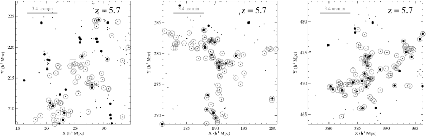
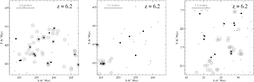
Figure 19: Close-up views of three $(20~{}h^{-1})^{3}$ Mpc³ regions that were found to be highly overdense in $z_{850}$$<$26.5 mag $i_{775}$-dropouts as marked by the squares in Fig. 18. The top row of panels correspond to the three richest regions found at $z=5.7$, while the bottom row corresponds to those at $z=6.2$. The position of the most massive halo in each region is indicated by a green square. Large and small dots correspond to dropout galaxies having $z_{850}$$<$26.5 and $<$27.5 mag, respectively. Galaxies that have been identified as part of a protocluster structure are indicated by blue circles. The scale bar at the top left in each panel corresponds to the size of an ACS/WFC pointing used to observe $z\sim 6$ QSO fields. Note that the galaxy corresponding to the most massive halo as indicated by the green square is not always detected in our $i_{775}$-dropout survey due to dust obscuration associated with very high star formation rates.

We can therefore conclude that the relatively average number of counts observed in the QSO fields is not inconsistent with the QSOs being hosted by very massive halos. However, one could make an equally strong case that they are, in fact, not. If we translate our results of Fig. 18 to the QSO fields that cover a smaller projected area of $(\sim 5~{}h^{-1})^{2}$ Mpc², and we add back in the average counts from the fore- and background provided by our lightcone data, we estimate that for QSOs at $z\approx 5.7$ we require an overdensity of $\delta_{\Sigma,ACS}\sim 4$ in order to be able to put a lower limit on the QSO host mass of $\sim 10^{12}$ $M_{\odot}$, while a $\delta_{\Sigma,ACS}\sim 1$ is consistent with $\sim 10^{11}$ $M_{\odot}$. At $z=6.2$, we would require $\delta_{\Sigma,ACS}\gtrsim 2$ for $M\gtrsim 10^{12}$ $M_{\odot}$ and $\delta_{\Sigma,ACS}\gtrsim 1$ for $M\gtrsim 10^{11.5}$ $M_{\odot}$. Comparison with the relatively low surface overdensities observed thus suggests that the halo mass is uncontrained by the current data. Nonetheless, we can at least conclude quite firmly that the QSOs are in far less rich environments (in terms of galaxy neigbours) compared to many rich regions found both in the simulations and in some of the deep field surveys described in the previous Section. In order to get a feel for what the QSO fields might have looked like if they were in highly overdense regions, we present some close-up views in Fig. 19 of the three richest regions of $z_{850}$$<$26.5 mag $i_{775}$-dropouts as marked by the small squares in Fig. 18. The central position corresponding to that of the most massive halo in each region is indicated by the green square. Large and small dots correspond to dropout galaxies having $z_{850}$$<$26.5 and $<$27.5 mag, respectively. For reference, we use blue circles to indicate galaxies that have been identified as part of a protocluster structure. The scale bar at the top left in each panel corresponds to the size of an ACS/WFC pointing used to observe $z\sim 6$ QSO fields. We make a number of interesting observations. First, using the current observational limits on depth ($z_{850}$=26.5 mag) and field size (3.4′, see scale bar) imposed by the ACS observations of QSOs, it would actually be quite easy to miss some of these structures as they typically span a larger region of 2–3 ACS fields in diameter. Going too much fainter magnitudes would help considerably, but this is at present unfeasible. Note, also, that in three of the panels presented here, the galaxy associated with the massive central halo does not pass our magnitude limits. It is missed due to dust obscuration associated with very high star formation rates inside these halos, implying that they will be missed by large-area UV searches as well (unless, of course, they also host a luminous, unobscured QSO).

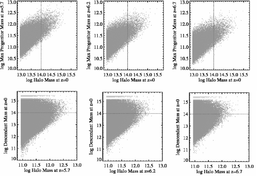
Figure 20: The correspondence between the most massive halos selected at $z=0$ and $z=6$ (see also Trenti et al., 2008). In the top row of panels we plot the mass of the most massive progrenitor of halos selected at $z=0$ for snapshots at $z=5.7$ (left), $z=6.2$ (middle) and $z=6.7$ (right). In the bottom row of panels we plot the mass of the most massive $z=0$ descendant for halos selected at $z=5.7$ (left), $z=6.2$ (middle) and $z=6.7$ (right). In all panels the dotted line indicates the mass corresponding to the threshold we use to define clusters at $z=0$ ($M\geq 10^{14}$ $h^{-1}$ $M_{\odot}$ Mpc). The dispersion in the mass of the most massive $z\sim 6$ progenitors of $z=0$ clusters is over an order of magnitude. Conversely, the most massive halos present at $z\sim 6$ are not necessarily the most massive halos at $z=0$, and a minority does not even pass the threshold imposed for qualifying as a $z=0$ cluster.

Finally, we investigate the level of mutual correspondence between the most massive halos selected at $z=6$ and $z=0$. In Fig. 19 we already saw that the richest regions are associated with a very large number of galaxies that will become part of a cluster when evolved to $z=0$. In the top row of Fig. 20 we show the mass of the most massive progenitors at $z=5.7$ (left), $z=6.2$ (middle) ad $z=6.7$ (right) of halos selected at $z=0$ (see also Trenti et al., 2008). The dotted line indicates the threshold corresponding to massive galaxy clusters at $z=0$. Although the progenitor mass increases systematically with increasing local mass, the dispersion in the mass of the most massive $z\sim 6$ progenitors is about or over one order of magnitude, and this is true even for the most massive clusters. As explained in detail by Trenti et al. (2008) this observation leads to an interesting complication when using the refinement technique often used to simulate the most massive regions in the early Universe by resimulating at high redshift the most massive region identified at $z=0$ in a coarse grid simulation. In the bottom panels of Fig. 20 we show the inverse relation between the most massive halos selected at $z\sim 6$ and their most massive descendant at $z=0$. From this it becomes clear that eventhough the most massive $z\sim 6$ halos (e.g. those associated with QSOs) are most likely to end up in present-day clusters, some evolve into only modest local structures more compatible with, e.g., galaxy groups. This implies that the present-day descendants of some of the first, massive galaxies and supermassive black holes must be sought in sub-cluster environments.

6 Discussion

Although our findings of the previous Section show that the apparent lack of excess neighbour counts near $z\sim 6$ QSOs is not inconsistent with them being hosted by supermassive dark matter halos as suggested by their low co-moving abundance and large inferred black hole mass, it is interesting to note that none of the QSO fields have densities that would place them amongst the richest structures in the $z\sim 6$ Universe. This leads to an intriguing question: where is the large-scale structure associated with QSOs?

One possibility that has been discussed (e.g. Kim et al., 2008) is that while the dark matter density near the QSOs is significantly higher compared to other fields, the strong ionizing radiation from the QSO may prohibit the condensation of gas thereby suppressing galaxy formation. Although it is not clear how important such feedback processes are exactly, we have found that proto-clusters in the MR form inside density enhancements that can extend up to many tens of Mpc in size. Although we do not currently know whether the $z\sim 6$ QSOs might be associated with overdensities on scales larger than a few arcminutes as probed by the ACS, it is unlikely that the QSO ionization field will suppress the formation of galaxies on such large scales (Wyithe et al., 2005). An alternative, perhaps more likely, explanation for the deficit of $i_{775}$-dropouts near QSOs, is that the dark matter halo mass of the QSOs is being greatly overestimated. Willott et al. (2005) suggest that the combination of the steepness of the halo mass function for rare high redshift halos on one hand, combined with the sizeable intrinsic scatter in the correlation between black hole mass and stellar velocity dispersion or halo mass at low redshift on the other hand, makes it much more probable that a $10^{9}$ $M_{\odot}$ black hole is found in relatively low mass halos than in a very rare halo of extremely high mass. Depending on the exact value of the scatter, the typical mass of a halo hosting a $z\sim 6$ QSO may be reduced by $\sim 0.5-1.5$ in log $\cal{M}$_halo without breaking the low redshift $\cal{M}$–$\sigma_{v}$ relation. The net result is that QSOs occur in some subset of halos found in substantially less dense environments, which may explain the observations. This notion seems to be confirmed by the low dynamical mass of $\sim 5\times 10^{10}$ $M_{\odot}$ estimated for the inner few kpc region of SDSS J1148+5251 at $z=6.43$ based on the CO line emission (Walter et al., 2004). This is in complete contradiction to the $\sim 10^{12}$ $M_{\odot}$ stellar mass bulges and $\sim 10^{13}$ $M_{\odot}$ mass halos derived based on other arguments. If true, models should then explain why the number density of such QSOs is as observed. On the other hand, recent theoretical work by Dijkstra et al. (2008) suggests that in order to facilitate the formation of a supermassive ($\sim 10^{9}$ $M_{\odot}$) by $z\sim 6$ in the first place, it may be required to have a rare pair of dark matter halos ($\sim 10^{13}$ $M_{\odot}$) in which the intense UV radiation from one halo prevents fragmentation of the other so that the gas collapses directly into a supermassive blackhole. This would constrain the QSOs to lie in even richer environments.

7 Recommendations for future observations

The predicted large-scale distributions of $i_{775}$-dropouts and Ly$\alpha$ emitters as shown in, e.g., Figs. 8, 15 and 16 show evidence for variations in the large-scale structure on scales of up to $\sim$1-2°, far larger than currently probed by deep HST or large-area ground-based surveys. A full appreciation of such structures could be important for a range of topics, including studies of the luminosity function at $z\sim 6$ and studies of the comparison between $\Lambda$CDM predictions and gravitational clustering on very large scales. The total area probed by our simulation is a good match to a survey of $\simeq 20$ degree² targeting $i_{775}$-dropouts and Ly$\alpha$ emitters at $z\sim 6$ planned with the forthcoming Subaru/HyperSurpimeCam (first light expected 2013; M. Ouchi, private communications, 2008).

We found that the $i_{775}$-dropouts associated with proto-clusters are almost exclusively found in regions with positive density enhancements. A proper understanding of such dense regions may also be very important for studies of the epoch of reionization. Simulations suggest that even though the total number of ionizing photons is much larger in very large proto-cluster regions covering several tens of comoving Mpc as compared to the field (e.g. Ciardi et al., 2003, but see Iliev et al. (2006)), they may still be the last to fully re-inionize, because the recombination rates are also much higher. If regions associated with QSOs or other structures were to contain significant patches of neutral hydrogen, this may affect both the observed number densities and clustering of LBGs or Ly$\alpha$ emitters relative to our assumed mean attenuation (McQuinn et al., 2007). However, since our work mostly focuses on $z\approx 6$ when reionization is believed to be largely completed, this may not be such an issue compared to surveys that probe earlier times at $z\gtrsim 7$ (e.g. Kashikawa et al., 2006; McQuinn et al., 2007).

Our evaluation of the possible structures associated with QSOs leads to several suggestions for future observations. While it is unlikely that the Wide Field Camera 3 (WFC3) to be installed onboard HST in early 2009 will provide better contraints than HST/ACS due to its relatively small field-of-view, we have shown that either by surveying a larger area of $\sim$10′$\times$10′ or by going deeper by $\sim$1 mag in $z_{850}$, one significantly reduces the shot noise in the neighbour counts allowing more reliable overdensities and (lower) limits on the halo masses to be estimated. A single pointing with ACS would require $\sim 15-20$ orbits in $z_{850}$ to reach a point source sensitivity of 5$\sigma$ for a $z_{850}$=27.5 mag object at $z\sim 6$. Given the typical structure sizes of the overdense regions shown in Fig. 19, a better approach would perhaps be to expand the area of the current QSO fields by several more ACS pointings at their present depth of $z_{850}$=26.5 mag for about an equal amount of time. However, this may be achieved from the ground as well using the much more efficient wide-field detector systems. Although this has been attempted by Willott et al. (2005) targeting three of the QSO fields, we note that their achieved depth of $z_{850}$=25.5 was probably much too shallow to find any overdensities even if they are there. We would like to stress that it is extremely important that foreground contamination is reduced as much as possible, for example by combining the observations with a deep exposure in the $V_{606}$ band. This is currently not available for the QSO fields, making it very hard to calculate the exact magnitude of any excess counts present. While a depth of $z_{850}$=27.5 mag seems out of reach for a statistical sample with HST, narrow-band Ly$\alpha$ surveys targeting the typically UV-faint Ly$\alpha$ emitters from the ground would be a very efficient alternative. Although a significant fraction of sources lacking Ly$\alpha$ may be lost compared to dropout surveys, they have the clear additional advantage of redshift information. Most Ly$\alpha$ surveys are carried out in the atmospheric transmission windows that correspond to redshifted Ly$\alpha$ either at $z\approx 5.7$ or $z\approx 6.6$ for which efficient narrow-band filters exist. We therefore suggest that the experiment is most likely to succeed around QSOs at $z\approx 5.7$ rather than the QSOs at $z\simeq 5.8-6.4$ looked at so far. It is, however, possible to use combinations of, e.g., the $z\approx 5.7$ narrow-band filter with medium or broad band filters at $\sim$9000Å to place stronger constaints on the photometric redshifts of $i_{775}$-dropouts in QSO fields (e.g., see Ajiki et al., 2006).

In the next decade, JWST will allow for some intriguing further possibilities that may provide some definite answers: Using the target 0.7–0.9$\mu$m sensitivity of the Near Infrared Camera (NIRCam) on JWST we could reach point sources at 10$\sigma$ as faint as $z_{850}$=28.5 mag in a 10,000 s exposure, or we could map a large $\sim$10′$\times$10′ region around QSOs to a depth of $z_{850}$=27.5 mag within a few hours. The Near Infrared Spectrograph (NIRSpec) will allow $>$100 simultaneous spectra to confirm the redshifts of very faint line or continuum objects over a $>$9 arcmin² field of view.

8 Summary

The main findings of our investigation can be summarized as follows.

$\bullet$ We have used the $N$-body plus semi-analytic modeling of De Lucia & Blaizot (2007) to construct the largest (4$\degr\times 4\degr$) mock galaxy redshift survey of star-forming galaxies at $z\sim 6$ to date. We extracted large samples of $i_{775}$-dropouts and Ly$\alpha$ emitters from the simulated survey, and showed that the main observational (colours, number densities, redshift distribution) and physical properties ($M_{*}$, SFR, age, $M_{halo}$) are in fair agreement with the data as far as they are constrained by various surveys.

$\bullet$ The present-day descendants of $i_{775}$-dropouts (brighter than $M^{*}_{UV,z=6}$) are typically found in group environments at $z=0$ (halo masses of a few times $10^{13}$ $M_{\odot}$). About one third of all $i_{775}$-dropouts end up in halos corresponding to clusters, implying that the contribution of “proto-cluster galaxies” in typical $i_{775}$-dropout surveys is significant.

$\bullet$ The projected sky distribution shows significant variations in the local surface density on scales of up to 1$\degr$, indicating that the largest surveys to date do not yet probe the full range of scales predicted by our $\Lambda$CDM models. This may be important for studies of the luminosity function, galaxy clustering, and the epoch of reionization.

$\bullet$ We present counts-in-cells frequency distributions of the number of objects expected per 3.4′$\times$3.4′ HST/ACS field of view, finding good agreement with the GOODS field statistics. The largest positive deviations are due to structures associated with the seeds of massive clusters of galaxies (“protoclusters”). To guide the interpretation of current and future HST/ACS observations, we give the probabilities of randomly finding regions of a given surface overdensity depending on the presence or absence of a protocluster.

$\bullet$ We give detailed examples of the structure of proto-cluster regions. Although the typical separation between protocluster galaxies does not reach beyond $\sim$10′ (25 Mpc comoving), they sit in overdensities that extend up to 30′ radius, indicating that the proto-clusters predominantly form deep inside the largest filamentary structures. These regions are very similar to two proto-clusters of $i_{775}$-dropouts or Ly$\alpha$ emitters found in the SDF (Ota et al., 2008) and SXDF (Ouchi et al., 2005) fields.

$\bullet$ We have made a detailed comparison between the number counts predicted by our simulation and those measured in fields observed with HST/ACS towards luminous $z\sim 6$ QSOs from SDSS, concluding that the observed fields are not particularly overdense in neighbour counts. We demonstrate that this does not rule out that the QSOs are in the most massive halos at $z\sim 6$, although we can also not confirm it. We discuss the possible reasons and implications of this intriguing result (see the Discussion in Section 6).

$\bullet$ We give detailed recommendations for follow-up observations using current and future instruments that can be used to better constrain the halo masses of $z\sim 6$ QSOs and the variations in the large-scale structure as probed by $i_{775}$-dropouts and Ly$\alpha$ emitters (see Section 7).

Table 1: Overview of $i$-dropout surveys.

Field Name	Survey Area	$z$-band detection limita	Reference
	(arcmin2)	(AB mag)
MR mock	70,000	$\sim$27.5	This paper
HUDF	11.2	$\sim$29.2 ($10\sigma$,$0\aas@@fstack{\prime\prime}2$)	Bouwens et al. (2006)
HUDF05	20.2	$\sim$28.9 ($5\sigma$,$0\aas@@fstack{\prime\prime}2$)	Bouwens et al. (2007); Oesch et al. (2007)
HUDF-Ps	17.0	$\sim$28.5 ($10\sigma$,$0\aas@@fstack{\prime\prime}2$)	Bouwens et al. (2006)
GOODS	316	$\sim$27.5 ($10\sigma$,$0\aas@@fstack{\prime\prime}2$)	Bouwens et al. (2006)
ACS/GTO	46	$\sim$27.3 ($6\sigma$,$1\aas@@fstack{\prime\prime}5$)	Bouwens et al. (2003)
SDF	876	$\sim$26.6 ($3\sigma$,$2\aas@@fstack{\prime\prime}0$)	Kashikawa et al. (2004)
SXDF	$\sim$4,680	$\sim$25.9 ($5\sigma$,$2\aas@@fstack{\prime\prime}0$)	Ota et al. (2005)
UKIDSS UDS + SXDF	$\sim$2,160	$\sim$25.0 ($5\sigma$,$2\aas@@fstack{\prime\prime}0$)	McLure et al. (2006)
QSO SDSSJ0836+0054 ($z=5.82$)	11.5	$\sim$26.5 ($5\sigma$,$0\aas@@fstack{\prime\prime}2$)	Zheng et al. (2006); Ajiki et al. (2006)
QSO SDSSJ1306+0356 ($z=5.99$)	$\sim$11.5	$\sim$26.5 ($5\sigma$,$0\aas@@fstack{\prime\prime}2$)	Kim et al. (2008)
QSO SDSSJ1630+4012 ($z=6.05$)	$\sim$11.5	$\sim$26.5 ($5\sigma$,$0\aas@@fstack{\prime\prime}2$)	Kim et al. (2008)
QSO SDSSJ1048+4637 ($z=6.23$)	$\sim$30	$\sim$26.2 ($3\sigma$,$1\aas@@fstack{\prime\prime}5$)	Willott et al. (2005)
	$\sim$11.5	$\sim$26.5 ($5\sigma$,$0\aas@@fstack{\prime\prime}2$)	Kim et al. (2008)
QSO SDSSJ1030+0524 ($z=6.28$)	$\sim$30	$\sim$26.2 ($3\sigma$,$1\aas@@fstack{\prime\prime}5$)	Willott et al. (2005)
	11.5	$\sim$26.5 ($5\sigma$,$0\aas@@fstack{\prime\prime}2$)	Stiavelli et al. (2005); Kim et al. (2008)
QSO SDSSJ1148+5251 ($z=6.43$)	$\sim$30	$\sim$26.2 ($3\sigma$,$1\aas@@fstack{\prime\prime}5$)	Willott et al. (2005)
	$\sim$11.5	$\sim$26.5 ($5\sigma$,$0\aas@@fstack{\prime\prime}2$)	Kim et al. (2008)

^a The numbers between parentheses correspond to the significance and the diameter of a circular aperture.

Table 2: $i$-dropout surface densities in the MR mock survey and observations.

	Surface Density (arcmin-2)
Magnitude	MR	MR	MR	MR	MR	B07a	O08a
	(total area)	(876 arcmin2)	(320 arcmin2)	(160 arcmin2)	(11.5 arcmin2)
$z^{\prime}<27.50$	2.31	$2.36\pm 0.31$	$2.31\pm 0.45$	$2.31\pm 0.52$	$2.28\pm 0.98$	$2.18\pm 0.23$
$z^{\prime}<27.00$	0.64	$0.62\pm 0.11$	$0.63\pm 0.15$	$0.64\pm 0.17$	$0.63\pm 0.38$	$0.83\pm 0.09$
$z^{\prime}<26.50$	0.18	$0.17\pm 0.03$	$0.18\pm 0.04$	$0.16\pm 0.06$	$0.18\pm 0.15$	$0.33\pm 0.04$	$\sim$0.18
$z^{\prime}<26.00$	0.08	$0.08\pm 0.01$	$0.08\pm 0.02$	$0.08\pm 0.03$	$0.08\pm 0.09$	$0.10\pm 0.02$	$\sim$0.11
$z^{\prime}<25.50$	0.04	$0.04\pm 0.01$	$0.05\pm 0.01$	$0.04\pm 0.02$	$0.04\pm 0.06$	$0.03\pm 0.01$	$\sim$0.04
$z^{\prime}<25.00$	0.03	$0.03\pm 0.01$	$0.03\pm 0.01$	$0.03\pm 0.01$	$0.03\pm 0.05$	$0.003\pm 0.003$	$\sim$0.01

^aObserved surface densities from Bouwens et al. (2007) and Ota et al. (2008).

References

- Ajiki et al. (2006) Ajiki, M., et al. 2006, PASJ, 58, 113
- Barth et al. (2003) Barth, A. J., Martini, P., Nelson, C. H., & Ho, L. C. 2003, ApJL, 594, L95
- Beers et al. (1990) Beers, T. C., Flynn, K., & Gebhardt, K. 1990, AJ, 100, 32
- Bertoldi et al. (2003) Bertoldi, F., et al. 2003, A&A, 409, L47
- Begelman et al. (2006) Begelman, M. C., Volonteri, M., & Rees, M. J. 2006, MNRAS, 370, 289
- Blaizot et al. (2005) Blaizot, J., Wadadekar, Y., Guiderdoni, B., Colombi, S. T., Bertin, E., Bouchet, F. R., Devriendt, J. E. G., & Hatton, S. 2005, MNRAS, 360, 159
- Bouwens et al. (2003) Bouwens, R. J., et al. 2003, ApJ, 595, 589
- Bouwens et al. (2004a) Bouwens, R. J., et al. 2004a, ApJL, 606, L25
- Bouwens et al. (2006) Bouwens, R. J., Illingworth, G. D., Blakeslee, J. P., & Franx, M. 2006, ApJ, 653, 53
- Bouwens et al. (2007) Bouwens, R. J., Illingworth, G. D., Franx, M., & Ford, H. 2007, ApJ, 670, 928
- Bouwens et al. (2004b) Bouwens, R. J., Illingworth, G. D., Blakeslee, J. P., Broadhurst, T. J., & Franx, M. 2004b, ApJL, 611, L1
- Bruzual & Charlot (2003) Bruzual, G., & Charlot, S. 2003, MNRAS, 344, 1000
- Calzetti (2001) Calzetti, D. 2001, PASP, 113, 1449
- Ciardi et al. (2003) Ciardi, B., Stoehr, F., & White, S. D. M. 2003, MNRAS, 343, 1101
- Croton et al. (2006) Croton, D. J., et al. 2006, MNRAS, 365, 11
- Davé et al. (2006) Davé, R., Finlator, K., & Oppenheimer, B. D. 2006, MNRAS, 370, 273
- De Lucia et al. (2004) De Lucia, G., Kauffmann, G., & White, S. D. M. 2004, MNRAS, 349, 1101
- De Lucia & Blaizot (2007) De Lucia, G., & Blaizot, J. 2007, MNRAS, 375, 2
- Dickinson et al. (2004) Dickinson, M. et al. 2004, ApJL, 600, L99
- Djorgovski et al. (2003) Djorgovski, S. G., Stern, D., Mahabal, A. A., & Brunner, R. 2003, ApJ, 596, 67
- Dow-Hygelund et al. (2005) Dow-Hygelund, C. C., et al. 2005, ApJL, 630, L137
- Dijkstra et al. (2008) Dijkstra, M., et al. 2008, MNRAS, submitted (arXiv:0810.0014)
- Eyles et al. (2007) Eyles, L. P., Bunker, A. J., Ellis, R. S., Lacy, M., Stanway, E. R., Stark, D. P., & Chiu, K. 2007, MNRAS, 374, 910
- Fan et al. (2003) Fan, X., et al. 2003, AJ, 125, 1649
- Fan et al. (2006b) Fan, X., et al. 2006b, AJ, 132, 117
- Fan et al. (2006a) Fan, X., et al. 2006a, AJ, 131, 1203
- Fan et al. (2004) Fan, X., et al. 2004, AJ, 128, 515
- Fan et al. (2001) Fan, X., et al. 2001, AJ, 122, 2833
- Finlator et al. (2007) Finlator, K., Davé, R., & Oppenheimer, B. D. 2007, MNRAS, 376, 1861
- Gayler Harford & Gnedin (2006) Gayler Harford, A., & Gnedin, N. Y. 2006, Submitted to ApJ (astro-ph/0610057)
- Goto (2006) Goto, T. 2006, MNRAS, 371, 769
- Gunn & Peterson (1965) Gunn, J. E., & Peterson, B. A. 1965, ApJ, 142, 1633
- Guo & White (2008) Guo, Q., & White, S. D. M. 2008, arXiv:0809.4259
- Haiman & Loeb (2001) Haiman, Z., & Loeb, A. 2001, ApJ, 552, 459
- Iliev et al. (2006) Iliev, I. T., Mellema, G., Pen, U.-L., Merz, H., Shapiro, P. R., & Alvarez, M. A. 2006, MNRAS, 369, 1625
- Jiang et al. (2007) Jiang, L., Fan, X., Vestergaard, M., Kurk, J. D., Walter, F., Kelly, B. C., & Strauss, M. A. 2007, AJ, 134, 1150
- Jiang et al. (2006) Jiang, L., et al. 2006, AJ, 132, 2127
- Kauffmann et al. (1999) Kauffmann, G., Colberg, J. M., Diaferio, A., & White, S. D. M. 1999, MNRAS, 303, 188
- Kashikawa et al. (2004) Kashikawa, N., et al. 2004, PASJ, 56, 1011
- Kashikawa et al. (2006) Kashikawa, N., et al. 2006, ApJ, 648, 7
- Kashikawa et al. (2007) Kashikawa, N., Kitayama, T., Doi, M., Misawa, T., Komiyama, Y., & Ota, K. 2007, ApJ, 663, 765
- Khochfar et al. (2007) Khochfar, S., Silk, J., Windhorst, R. A., & Ryan, R. E., Jr. 2007, ApJL, 668, L115
- Kitzbichler & White (2007) Kitzbichler, M. G., & White, S. D. M. 2007, MNRAS, 376, 2
- Kim et al. (2008) Kim, S., et al. 2008, ArXiv e-prints, 805, arXiv:0805.1412
- Kurk et al. (2007) Kurk, J. D., et al. 2007, ArXiv e-prints, 707, arXiv:0707.1662
- Lai et al. (2007) Lai, K., Huang, J.-S., Fazio, G., Cowie, L. L., Hu, E. M., & Kakazu, Y. 2007, ApJ, 655, 704
- Lemson & Virgo Consortium (2006) Lemson, G., & Virgo Consortium, t. 2006, e-print (arXiv:astro-ph/0608019)
- Lemson & Springel (2006) Lemson, G., & Springel, V. 2006, Astronomical Data Analysis Software and Systems XV, 351, 212
- Li et al. (2007) Li, Y., et al. 2007, ApJ, 665, 187
- Madau (1995) Madau, P. 1995, ApJ, 441, 18
- Madau et al. (1998) Madau, P., Pozzetti, L., & Dickinson, M. 1998, ApJ, 498, 106
- Malhotra et al. (2005) Malhotra, S., et al. 2005, ApJ, 626, 666
- Maiolino et al. (2005) Maiolino, R., et al. 2005, A&A, 440, L51
- Magorrian et al. (1998) Magorrian, J., et al. 1998, AJ, 115, 2285
- McLure et al. (2008) McLure, R. J., Cirasuolo, M., Dunlop, J. S., Foucaud, S., & Almaini, O. 2008, ArXiv e-prints, 805, arXiv:0805.1335
- McLure et al. (2006) McLure, R. J., et al. 2006, MNRAS, 372, 357
- McQuinn et al. (2007) McQuinn, M., Hernquist, L., Zaldarriaga, M., & Dutta, S. 2007, MNRAS, 381, 75
- Miley et al. (2004) Miley, G. K., et al. 2004, Nature, 427, 47
- Monaco et al. (2005) Monaco, P., Møller, P., Fynbo, J. P. U., Weidinger, M., Ledoux, C., & Theuns, T. 2005, A&A, 440, 799
- Muñoz & Loeb (2008a) Muñoz, J. A., & Loeb, A. 2008a, MNRAS, 385, 2175
- Muñoz & Loeb (2008b) Muñoz, J. A., & Loeb, A. 2008b, MNRAS, 386, 2323
- Narayanan et al. (2007) Narayanan, D., et al. 2007, ArXiv e-prints, 707, arXiv:0707.3141
- Nagamine et al. (2006) Nagamine, K., Cen, R., Furlanetto, S. R., Hernquist, L., Night, C., Ostriker, J. P., & Ouchi, M. 2006, New Astronomy Review, 50, 29
- Nagamine et al. (2008) Nagamine, K., Ouchi, M., Springel, V., & Hernquist, L. 2008, ApJ, submitted (arXiv:0802.0228)
- Night et al. (2006) Night, C., Nagamine, K., Springel, V., & Hernquist, L. 2006, MNRAS, 366, 705
- Oesch et al. (2007) Oesch, P. A., et al. 2007, ApJ, 671, 1212
- Ota et al. (2008) Ota, K., Kashikawa, N., Malkan, M. A., Iye, M., Nakajima, T., Nagao, T., Shimasaku, K., & Gandhi, P. 2008, ArXiv e-prints, 804, arXiv:0804.3448
- Ota et al. (2005) Ota, K., Kashikawa, N., Nakajima, T., & Iye, M. 2005, Journal of Korean Astronomical Society, 38, 179
- Ouchi et al. (2004) Ouchi, M., et al. 2004, ApJ, 611, 685
- Ouchi et al. (2005) Ouchi, M., et al. 2005, ApJL, 620, L1
- Overzier et al. (2006) Overzier, R. A., Bouwens, R. J., Illingworth, G. D., & Franx, M. 2006, ApJL, 648, L5
- Overzier et al. (2008a) Overzier, R. A., et al. 2008a, ApJ, 677, 37
- Overzier et al. (2008b) Overzier, R. A., et al. 2008b, ApJ, 673, 143
- Priddey et al. (2007) Priddey, R. S., Ivison, R. J., & Isaak, K. G. 2007, ArXiv e-prints, 709, arXiv:0709.0610
- Robertson et al. (2007) Robertson, B., Li, Y., Cox, T. J., Hernquist, L., & Hopkins, P. F. 2007, ApJ, 667, 60
- Shimasaku et al. (2003) Shimasaku, K., et al. 2003, ApJL, 586, L111
- Shimasaku et al. (2005) Shimasaku, K., Ouchi, M., Furusawa, H., Yoshida, M., Kashikawa, N., & Okamura, S. 2005, PASJ, 57, 447
- Springel (2005b) Springel, V. 2005b, MNRAS, 364, 1105
- Spergel et al. (2003) Spergel, D. N., et al. 2003, ApJS, 148, 175
- Springel et al. (2005a) Springel, V., et al. 2005a, Nature, 435, 629
- Stanway et al. (2003) Stanway, E. R., Bunker, A. J., & McMahon, R. G. 2003, MNRAS, 342, 439
- Stiavelli et al. (2005) Stiavelli, M., et al. 2005, ApJL, 622, L1
- Steidel et al. (2005) Steidel, C. C., Adelberger, K. L., Shapley, A. E., Erb, D. K., Reddy, N. A., & Pettini, M. 2005, ApJ, 626, 44
- Steidel et al. (1998) Steidel, C. C., Adelberger, K. L., Dickinson, M., Giavalisco, M., Pettini, M., & Kellogg, M. 1998, ApJ, 492, 428
- Stanway et al. (2007) Stanway, E. R., et al. 2007, MNRAS, 376, 727
- Suwa et al. (2006) Suwa, T., Habe, A., & Yoshikawa, K. 2006, ApJL, 646, L5
- Trenti et al. (2008) Trenti, M., Santos, M. R., & Stiavelli, M. 2008, ArXiv e-prints, 807, arXiv:0807.3352
- Venemans et al. (2007) Venemans, B. P., McMahon, R. G., Warren, S. J., Gonzalez-Solares, E. A., Hewett, P. C., Mortlock, D. J., Dye, S., & Sharp, R. G. 2007, MNRAS, 376, L76
- Vestergaard (2004) Vestergaard, M. 2004, ApJ, 601, 676
- Venemans et al. (2007) Venemans, B. P., et al. 2007, A&A, 461, 823
- Volonteri & Rees (2006) Volonteri, M., & Rees, M. J. 2006, ApJ, 650, 669
- Walter et al. (2004) Walter, F., Carilli, C., Bertoldi, F., Menten, K., Cox, P., Lo, K. Y., Fan, X., & Strauss, M. A. 2004, ApJL, 615, L17
- Wang et al. (2007) Wang, R., et al. 2007, AJ, 134, 617
- Wang et al. (2008) Wang, J., De Lucia, G., Kitzbichler, M. G., & White, S. D. M. 2008, MNRAS, 384, 1301
- White (2001) White, M. 2001, A&A, 367, 27
- White et al. (2003) White, R. L., Becker, R. H., Fan, X., & Strauss, M. A. 2003, AJ, 126, 1
- Willott et al. (2005) Willott, C. J., Percival, W. J., McLure, R. J., Crampton, D., Hutchings, J. B., Jarvis, M. J., Sawicki, M., & Simard, L. 2005, ApJ, 626, 657
- Willott et al. (2003) Willott, C. J., McLure, R. J., & Jarvis, M. J. 2003, ApJL, 587, L15
- Wyithe et al. (2005) Wyithe, J. S. B., Loeb, A., & Carilli, C. 2005, ApJ, 628, 575
- Yan et al. (2006) Yan, H., Dickinson, M., Giavalisco, M., Stern, D., Eisenhardt, P. R. M., & Ferguson, H. C. 2006, ApJ, 651, 24
- Yan & Windhorst (2004a) Yan, H., & Windhorst, R. A. 2004a, ApJL, 612, L93
- Yan & Windhorst (2004b) Yan, H., & Windhorst, R. A. 2004b, ApJL, 600, L1
- Zentner (2007) Zentner, A. R. 2007, International Journal of Modern Physics D, 16, 763
- Zheng et al. (2006) Zheng, W., et al. 2006, ApJ, 640, 574