Real-time gauge theory simulations from stochastic quantization with optimized updating

Abstract

Stochastic quantisation is applied to the problem of calculating real-time evolution on a Minkowskian space-time lattice. We employ optimized updating using reweighting, or gauge fixing, respectively. These procedures do not affect the underlying theory, but strongly improve the stability properties of the stochastic dynamics.

1 Introduction

First-principles simulation of quantum field theories (such as QCD) is a notoriously hard problem of theoretical physics. Lattice calculations tipically use euclidean formulation, where one can apply importance sampling. In contrast, in Minkowski space, this is ineffective since the probability weight is in this case a phase factor: $\exp(iS).$ Stochastic quantisation [1], however can be generalised to complex weights. Recently stochastic quantisation was applied to calculate the real-time evolution of quantum fields ([2, 3] and references therein). Recently stochastic quantisation has also been applied to nonzero chemical potential problems [4]. In [5], optimized updatings were studied, which improve the behaviour of the complex Langevin equations, whitout changing the underlying theory. The main insight is the usage of the fixedpoints of the Langevin flow as a criteria for convergence.

2 Stochastic Quantisation

The time evolution can be formulated using the path integral formalism as an average weighted with $\exp(iS)$:

$$\langle O(\Phi)\rangle=\int D\Phi e^{iS}O(\Phi)$$ (1)

Using stochastic quantization the real-time quantum configurations in 3+1 dimensions are constructed by a stochastic process in an additional (5th) Langevin-time $\theta$, by use of a Langevin equation:

$${\partial\Phi(\theta)\over\partial\theta}=-i{\delta S\over\delta\Phi}+\eta(\theta)$$ (2)

where $\eta$, the noise term satisfies: $\langle\eta(\theta)\rangle=0,\ \langle\eta(\theta)\eta(\theta^{\prime})\rangle=2\delta(\theta-\theta^{\prime})$. The expectation value of any observable can be calculated from the Langevin-time evolution using the following formula:

$$\langle O(\Phi)\rangle={1\over T}\int_{0}^{T}O(\Phi(\theta))d\theta$$ (3)

We applied stochastic quantisation to “one plaquette” models, which serve to illustrate and test concepts of optimized updating, a scalar oscillator (0+1 dimensional scalar field theory), pure $SU(2)$ gauge theory, using the Wilson action on a 3+1 dimensional lattice. The field theories were discretised on a comlex time contour, which enabled us to either calculate equilibrium distributions, or non-equilibrium time evolution. The contour tipically has a downward slope, which improves convergence.

The complexity of the drift term in (2) means that the originally real fields are complexified. This transfroms a real scalar field to complex scalar, the link variables of an $SU(N)$ field theory to $SL(N,{\bf C})$. Only after taking noise or Langevin-time averages, respectively, the expectation values of the original real scalar theory ($SU(N)$ gauge theory) are to be recovered. Accordingly, if the Langevin flow converges to a fixed point solution of Eq. (2) it automatically fulfills the infinite hierarchy of Dyson-Schwinger identities of the original theory.

3 Optimized updating of toy models

As an example to illustrate reweighting we consider the one-plaquette model with $U(1)$ symmetry. For $U=e^{i\varphi}$ the action is given by

$$S_{0}\,=\,\frac{\beta}{2}\left(U+U^{-1}\right)\,=\,\beta\cos\varphi\,$$ (4)

with real coupling parameter $\beta$. This simple model enables us to check the results of the complex Langevin equation by evaluating the integral

$$\langle O\rangle_{0}\,=\,\frac{1}{Z_{0}}\int_{0}^{2\pi}{\rm d}\varphi\,\e^{iS_{0}}\,O(\varphi)\,.$$ (5)

For real $\beta$ the integrand in Eq. (5) is not positive definite, which mimics certain aspects of more complicated theories in Minkowskian space-time. Solving the discretised Langevin equation corresponding to this model, using $\beta=1$, and a Langevin stepsize $\epsilon=10^{-5}$, one gets:

$$\langle e^{i\varphi}\rangle_{0}\,\stackrel{{\scriptstyle\rm without\atop optimization}}{{=}}\,-0.009(\pm 0.006)-i\,0.00006(\pm 0.00007)\,.$$ (6)

Evaluating the numerical integral in (5), one gets $\langle e^{i\varphi}\rangle\simeq i0.575$. One observes that the simulation yields a wrong result that is compatible with zero, in contrast to the non-vanishing imaginary value obtained analytically.

The same averages may be calculated using by performing reweighting: changing the action, and recompensating the change in the measurable so that the end-result remains the same.

$$\langle O\rangle_{0}\,=\,\frac{\int_{0}^{2\pi}{\rm d}\varphi\,\e^{iS_{\alpha}}\,e^{i(S_{0}-S_{\alpha})}\,O(\varphi)}{\int_{0}^{2\pi}{\rm d}\varphi\,\e^{iS_{\alpha}}e^{i(S_{0}-S_{\alpha})}}$$ (7)

Evaluating the denominator and numerator of this factor one considers $S_{\alpha}$ as the action instead of $S_{0}$, thus the Langevin process is changed [5]. We will consider here the family of actions $S_{\alpha}=S_{0}+\alpha\varphi=\beta\cos\varphi+\alpha\varphi$. One finds that this new class of actions gives exact results for some region of its parameters (see Fig. 1), such that $\langle e^{i\varphi}\rangle_{0}$ is recoverable, using (7).

Figure 1: The real and imaginary part of the average $\langle e^{i\varphi}\rangle_{\alpha=1}$ as a function of $\beta$. The lines represent averages obtained from direct integration, while the symbols are measurements using a stochastic process.

Qualitative understanding of the behavior of stochastic processes corresponding to $S_{\alpha}$ is possible by studying the fixed point structure of the drift term of the Langevin equation. In Fig. 2. the flowchart (normalized drift vectors) is plotted alongside a scatter plot of $\varphi$ on the complex plane. One observes (comparing with Fig. 1) that the stochastic results brake down when the fixed point structure changes. Exact results correspond to an attractive fixedpoint, and a relatively compact distribution of field values, while the absence of attractive fixedpoints, and a wide distribution corresponds to the breakdown. The breakdown of the process using the original $S_{0}$ action is consistent with this picture: it has no attractive fixedpoints.

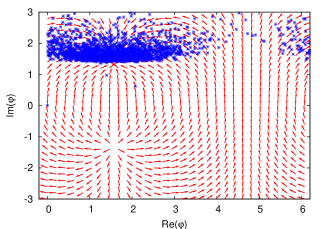
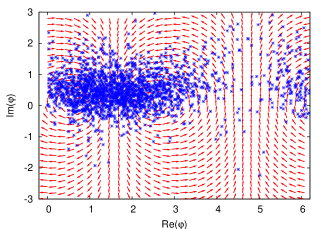
Figure 2: Shown is the real and imaginary part of $\partial S_{\alpha}/\partial\varphi$ plotted as a vector with origin at each $\varphi$-value and with normalized length for better visibility, using $\alpha=1$, and $\beta=0.5$ on the left panel and $\beta=1.5$ on the right panel. Also shown is the distribution of $\varphi$ as obtained from the full solution of the respective complex Langevin equation.

Consider now the $SU(2)$ one plaquette model, as a second example. The action is given by:

$$S(U)=\frac{\beta}{2}\,{\rm Tr}\,U\,,$$ (8)

which is invariant under the “gauge” transformation $U\rightarrow W^{-1}UW$ with $U,W\in SL(2,{\bf C})$ (after complexification).

Since the $SU(2)$ one-plaquette model has a global symmetry, one may use this symmetry to ”gauge-fix” certain variables in order to constrain the growth of fluctuations. In the following we will use it in order to diagonalize $U$ after each successive Langevin-time step: $U^{\prime}\,=\,{\rm diag}\left(a+i\sqrt{1-a^{2}},a-i\sqrt{1-a^{2}}\right)$ (for details, see [5]). The right graph of Fig. 3 shows that the ”gauge-fixing” leads to a compact distribution, and exact results, in contrast to the distribution from the unmodified process displayed on the left of that figure, which gives wrong results.

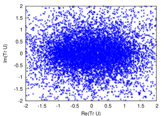
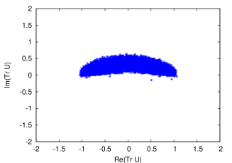
Figure 3: The real and imaginary part of the plaquette variable ${\rm Tr}U$ from snapshots with constant Langevin-time stepping for the $SU(2)$ one-plaquette model with $\beta=1$. The left graph shows the wide distribution of values obtained from the standard Langevin dynamics, while the right graph displays the compact distribution from the (”gauge-fixed”) optimized process (see text for explanation).

In conclusion, we have demonstrated the usage of optimized updating on specific examples, which change the Langevin process by reweighting or using the symmetries of the theory, in a way that it gives exact results for the original theory.

Acknowledgements: I would like to thank Jürgen Berges, Szabolcs Borsányi and Ion-Olimpiu Stamatescu for a fruitful collaboration on stochastic quantization.

References

- [1] G. Parisi and Y. s. Wu, Sci. Sin. 24 (1981) 483.
- [2] J. Berges and I. O. Stamatescu, Phys. Rev. Lett. 95 (2005) 202003 [arXiv:hep-lat/0508030].
- [3] J. Berges, S. Borsanyi, D. Sexty and I. O. Stamatescu, Phys. Rev. D 75 (2007) 045007 [arXiv:hep-lat/0609058].
- [4] G. Aarts and I. O. Stamatescu, JHEP 0809 (2008) 018 [arXiv:0807.1597 [hep-lat]].
- [5] J. Berges and D. Sexty, Nucl. Phys. B 799 (2008) 306 [arXiv:0708.0779 [hep-lat]].