A Catalog of Broad Absorption Line Quasars in Sloan Digital Sky Survey Data Release 5

Abstract

We present a catalog of 5039 broad absorption line (BAL) quasars (QSOs) in the Sloan Digital Sky Survey (SDSS) Data Release 5 (DR5) QSO catalog that have absorption troughs covering a continuous velocity range $\geq 2000$ km s^-1. We have fit ultraviolet (UV) continua and line emission in each case, enabling us to report common diagnostics of BAL strengths and velocities in the range $-25,000$ to $0$ km s^-1 for Si IV $\lambda$1400, C IV $\lambda$1549, Al III $\lambda$1857, and Mg II $\lambda$2799. We calculate these diagnostics using the spectrum listed in the DR5 QSO catalog, and also for spectra from additional SDSS observing epochs when available. In cases where BAL QSOs have been observed with Chandra or XMM-Newton, we report the X-ray monochromatic luminosities of these sources.

We confirm and extend previous findings that BAL QSOs are more strongly reddened in the rest-frame UV than non-BAL QSOs and that BAL QSOs are relatively X-ray weak compared to non-BAL QSOs. The observed BAL fraction is dependent on the spectral signal-to-noise (S/N); for higher-S/N sources, we find an observed BAL fraction of $\approx$15%. BAL QSOs show a similar Baldwin effect as for non-BAL QSOs, in that their C IV emission equivalent widths decrease with increasing continuum luminosity. However, BAL QSOs have weaker C IV emission in general than do non-BAL QSOs. Sources with higher UV luminosities are more likely to have higher-velocity outflows, and the BAL outflow velocity and UV absorption strength are correlated with relative X-ray weakness. These results are in qualitative agreement with models that depend on strong X-ray absorption to shield the outflow from over-ionization and enable radiative acceleration. In a scenario in which BAL trough shapes are primarily determined by outflow geometry, observed differences in Si IV and C IV trough shapes would suggest that some outflows have ion-dependent structure.

Accepted to ApJ. (c) Copyright 2008. The American Astronomical Society. All rights reserved. Printed in U.S.A.

1 INTRODUCTION

The study of broad absorption lines (BALs) commonly observed in the ultraviolet (UV) spectra of optically-selected quasars (QSOs; e.g., Trump et al., 2006, and references therein) significantly advances our understanding of the structure and emission/absorption physics of Active Galactic Nuclei (AGN). BALs are at least 2000 km s^-1 wide by definition (Weymann et al., 1991), and can be accelerated up to and beyond velocities of $0.1c$. The depth of absorption at a given outflow velocity is largely determined by the fraction of the UV emission region covered by the BAL outflow (e.g., Arav et al., 1999a, and see also Appendix A of Hall et al. (2002)), and is therefore an indicator of the outflow structure. In some cases, BAL troughs have been observed to change dramatically over several (rest-frame) years, indicating that the structure of the BAL outflow evolves on observable time scales (e.g., Gibson et al., 2008b). It is thought that an X-ray absorber shields the BAL outflow from overionization by the soft X-rays generated in the heart of the QSO so that UV radiation can accelerate the outflow to high velocities (e.g., Murray et al., 1995). The shielding X-ray absorber may also influence other BAL properties, such as the maximum outflow velocity (e.g., Gallagher et al., 2006).

BAL characteristics such as outflow velocities, velocity widths, and absorption depths vary widely among individual sources; large samples are therefore required in order to obtain a general understanding of QSO physics. Variability and multi-wavelength studies of BAL QSOs can be performed with dedicated observations, but are most economically conducted using publicly-archived, serendipitous observations of optically-identified BAL QSOs. Such studies have become possible due to large QSO surveys with well-understood selection properties that have greatly increased the number of known, representative BAL QSOs. Hewett & Foltz (2003) identified a sample of 67 BAL QSOs in the Large Bright Quasar Survey (LBQS; Hewett et al., 1995, and references therein). Tolea et al. (2002) and Reichard et al. (2003) studied 116 and 224 BAL QSOs, respectively, in the Sloan Digital Sky Survey (SDSS; York et al., 2000) Early Data Release (EDR). Ganguly et al. (2007) have identified $\approx$600 QSOs with broad absorption in SDSS Data Relase 2 (DR2), while Trump et al. (2006) have recently identified 1986 traditional BAL QSOs in the SDSS Data Release 3 (DR3) QSO catalog (Schneider et al., 2005). As survey technology progresses (e.g., from the LBQS to the SDSS), fainter sources are catalogued, increasing our coverage of the QSO luminosity/redshift plane. As a result, we are not only increasing sample sizes over time, but also increasing the physical parameter space for QSO studies.

In the current study, we identify and quantify the BAL absorption in sources in the SDSS DR5 QSO catalog (Schneider et al., 2007). Of the 77,429 DR5 QSOs in the catalog, we identify 4204 traditionally-defined BAL QSOs, 481 of which have BALs from low ionization stages of Al III and/or Mg II. Our sample size increases to 5039 BAL QSOs if we extend the traditional definition to include BALs that have absorption at outflow velocities within 3000 km s^-1 of the emission line redshift. (The “traditional” and “extended” BAL definitions are formally detailed in §2.) In cases where multiple SDSS spectra are publicly available for a QSO, we identify BALs present in the duplicate spectra as well as in the primary spectrum listed in the DR5 QSO catalog. We also determine the monochromatic X-ray luminosities of BAL QSOs that were observed with Chandra and/or XMM-Newton and test for any correlations between BAL properties and relative X-ray brightness.

Because conventions vary among studies, we briefly describe the terminology used in this catalog. BAL QSOs are broadly classified by ionization into low-ionization BAL QSOs (“LoBALs”) and high-ionization BAL QSOs (“HiBALs”). LoBALs are QSOs that have BALs from ions at lower ionization states such as Al III or Mg II. They may also have BALs from higher ionization stages such as Si IV or C IV. “FeLoBALs,” which show broad absorption from iron blueward of 2800 Å, are included in the category of LoBALs for this work. HiBALs have BALs only from high ionization stages. While most BAL QSOs do not have broad Al III or Mg II absorption lines, the unambiguous classification of HiBALs requires spectra that extend to the Al III and Mg II regions in order to verify that no BALs are present for these ions.

We define velocities flowing outward (with respect to QSO emission rest frames) to be negative. Positive velocities indicate features that are at longer wavelengths than the wavelength corresponding to (rest-frame) zero velocity. However, we use the terms “greater” and “smaller” velocities to refer to the magnitude of the velocity, so that an outflow velocity of –10,000 km s^-1 is “greater” than a velocity of –5000 km s^-1. We adopt this convention to match common terminology.

Throughout this work we use a cosmology in which $H_{0}=70$ km s^-1 Mpc^-1, $\Omega_{M}=0.3,$ and $\Omega_{\Lambda}=0.7$.

2 OBSERVATIONS AND DATA REDUCTION

This BAL catalog is constructed from SDSS Data Release 5 (Adelman-McCarthy et al., 2007). The SDSS uses a CCD camera (Gunn et al., 1998) on a dedicated 2.5 m telescope (Gunn et al., 2006) at Apache Point Observatory, New Mexico, to obtain images in five broad optical bands ($ugriz$; Fukugita et al., 1996) over approximately 10,000 deg² of the high Galactic latitude sky. The survey data-processing software measures the properties of each detected object in the imaging data in all five bands, and determines and applies both astrometric and photometric calibrations (Smith et al., 2002; Pier et al., 2003; Ivezić et al., 2004). The SDSS quasar target selection algorithm is presented in Richards et al. (2002). See Stoughton et al. (2002) for a detailed description of many of the technical aspects of the SDSS. The SDSS photometry is reported on the asinh magnitude scale (Lupton et al., 1999).

In order to account for the loss of flux due to “fiber leak,” we multiply each spectra by a constant that matches the photometric $g$, $r$, and $i$ PSF magnitudes to those synthesized from the spectra. In cases where the synthetic magnitudes are lower (brighter) than the PSF magnitudes (e.g., because the source luminosity has varied), we leave the spectrum unchanged. We also correct the spectra for Galactic extinction using the reddening curve of Cardelli et al. (1989) with the near-UV extension of O’Donnell (1994). We obtain $E(B-V)$ from the NASA Extragalactic Database (NED), which uses the dust maps of Schlegel et al. (1998). The redshifts for our QSOs are taken from the DR5 QSO catalog, with the exception of two sources, J$100424.88+122922.2$ and J$153029.05+553247.9$, which we consider to be misclassified. We assign these sources redshifts of 4.66 and 1.73, respectively.

We do not rebin SDSS spectra except in a few special cases for which we note the rebinning method directly. A “spectral bin” therefore refers to the standard wavelength binning of SDSS spectra, which is $\approx$69 km s^-1 per bin in the observing frame.

We fit SDSS spectra using the algorithm of Gibson et al. (2008b), which we summarize here. For QSOs at $z\geq 1.7$, our continuum model is a power law reddened using the Small Magellanic Cloud reddening curve of Pei (1992). For QSOs at lower redshifts, we use a fourth- or sixth-degree polynomial; in our experience this non-physical model is able to reproduce well the complex continuum at longer wavelengths. We initially fit regions that are generally free from strong absorption or emission features: 1250–1350, 1700–1800, 1950–2200, 2650–2710, 2950–3700, 3950–4050, 4140–4270, 4400–4800, 5100–6400, and $>$6900 Å. We then iteratively fit the continuum, ignoring at each step wavelength bins that deviate by $>$3$\sigma$ from the current fit in order to exclude strong absorption and emission features. We fit Voigt profiles to the strongest emission lines expected in the spectrum: Si IV $\lambda$1400, C IV $\lambda$1549, Al III $\lambda$1857, C III] $\lambda$1909, and Mg II $\lambda$2799. These wavelengths are taken from the SDSS vacuum wavelength list used by the SDSS pipeline to determine emission-line redshifts. The wavelengths of the emission lines are allowed to vary in the fit. We ascribe no physical significance to the Voigt profile; it simply enables us to model emission line cores and wings using a small number of parameters. We fit emission lines iteratively as well, ignoring at each step bins that are absorbed by more than $2.5\sigma$ from the continuum $+$ emission fit. Due to the degeneracy between the UV emission continuum shape and the magnitude of intrinsic reddening, we do not attach physical significance to the values of $E(B-V)$ obtained from our fits. The UV luminosities we report are therefore corrected for Galactic, but not intrinsic, reddening. After the initial automatic fits were performed, RRG inspected and manually adjusted the automatic fits. Other reviewers (LJ, YS, WNB, JW, PBH, SFA, DVB, DPS) then examined this adjusted sample of spectra in order to ensure that BALs were not missed or mis-characterized.

We smoothed each spectrum using a boxcar three bins wide and then searched the smoothed spectra for BALs by calculating $BI$, the traditional “balnicity index” of Weymann et al. (1991). The balnicity index is defined as

$$BI \equiv \int^{25,000}_{3000}\biggl{(}1-\frac{f(-v)}{0.9}\biggr{)}C~{}dv,$$ (1)

where $f(v)$ is the continuum-normalized spectral flux at a velocity $v$ (in km s^-1) from the line rest wavelength (in the system frame). The dimensionless value $C$ is $0$ unless the observed spectrum has fallen at least 10% below the continuum for a velocity width of at least 2000 km s^-1 on the red side of the absorption trough, at which point $C$ is set to $1$. Traditional BALs are defined to have $BI>0$. Because this metric does not include a large number of broad absorption features at lower outflow velocities, we also define and calculate $BI_{0}$ in a similar fashion to $BI$, but integrate to $0$ km s^-1 instead of $-3000$ km s^-1. We measure $BI$ and $BI_{0}$ for Si IV, C IV, Al III, and Mg II, using the wavelength for the red component of the doublets given in the theoretical line list of Verner et al. (1995) to define zero velocity for each ion. These wavelengths are 1402.77 Å (Si IV), 1550.77 Å (C IV), 1862.79 Å (Al III), and 2803.53 Å (Mg II). In some cases, BAL troughs may be contaminated by absorption from other ions, such as Fe II $\lambda$2632 and C II $\lambda$1335. Such contamination is difficult to identify except when strong absorption begins at the known wavelengths of these lines. In general, we do not account for contamination, but ascribe all broad absorption to Si IV, C IV, Al III, or Mg II. In §3, we list 92 sources in our BAL catalog that appear to have contaminated BALs, based on visual inspection.

Overall, our models are able to accurately reproduce the observed continuum and emission line features in the SDSS QSO spectra. However, there are cases where reproducing emission is problematic. This could occur, for example, if an emission line profile is highly asymmetric. There are also cases, such as strongly-absorbed emission line profiles, for which we were unable to accurately determine the underlying emission. We define a set of flags that we use to indicate when the fit model is particularly uncertain due to such effects.

1. EmLost: The profile of the emission line at (nearly) zero velocity has been strongly absorbed and may not have been accurately reconstructed. The EmLost flag is set if a BAL is found for this ion and either: the center of the (best-guess) emission line fit is in the BAL region, the FWHM of our (best-guess) emission line fit is $<$10 Å, or there is evidence that a broad range of spectral bins in the line center are absorbed. Quantitatively, for the last criterion, we require that at least 15 adjacent bins (20 for Mg II) fall $\geq$5% below our emission model fit, and these absorbed bins lie in the wavelength region where the emission is above the line half-maximum. Our fitting experience indicates that characterizing emission lines is particularly difficult in cases meeting these criteria. Low-velocity absorption is very common; nearly half of the sources with C IV $BI_{0}>0$ have this flag set for the C IV emission line. Setting this flag indicates that measurements of BAL troughs are less certain in cases where the BAL extends to low velocities.

2. BlueWingAbs: Additional “blue wing” emission occurs on the blue side of the C IV emission line, and absorption is apparent between the blue wing and the line core. Since we fit only the line core and cannot accurately reconstruct the “blue wing” emission, we could potentially miss BAL absorption in these cases. The BlueWingAbs flag is set to “1” when 15 consecutive bins redward of 1500 Å lie above the model fit, and 15 more consecutive bins further redward lie below the model, and all these bins are shortward of the wavelength at which the blue side of the C IV emission line reaches its half-maximum.

3. BALManyBadBins: Some putative BALs consist of a large number of spectral bins that have been flagged as “bad” in the SDSS pipeline. Unfortunately, the pipeline occasionally flags bins that are acceptable, and the low flux density and signal-to-noise (S/N) in BAL troughs make them especially susceptible to flagging. We report the BALManyBadBins flag when $>$25% of the bins in a BAL have been flagged by the SDSS. However, we ignore the flags BRIGHTSKY and EMLINE, because these warnings can be triggered by the low flux levels in strong BAL troughs.

Figure  1 shows examples of spectra that have the EmLost and BlueWingAbs flags set for the C IV absorption region.

The 2200–3000 Å region surrounding the Mg II emission line is especially difficult to model due to poorly-constrained emission line structure and blended emission from ions such as Fe II. Modeling the full emission structure in this region is beyond the scope of this study. For Mg II absorption, we have fit the emission line core and estimated the continuum model from the fit to the surrounding region. We therefore do not claim that our Mg II absorption list is complete, although visual inspections indicate that we have not missed a large number of strong, broad absorption features.

In some cases, we report BAL absorption detected in the observed spectrum even though the entire outflow velocity range (defined to be $-25,000$ to $0$ km s^-1) does not fall in the SDSS spectral bandpass. As a result, the reported BAL properties may not accurately represent the measurements that would be obtained if the full velocity range were observed. If a representative sample of BAL properties is required, redshift restrictions should be placed on QSO samples to ensure that the entire potential absorption region falls in the SDSS bandpass. We discuss this point further in §4.

Small, systematic misestimates of the true continuum level could cause us to miss or mistakenly identify broad, shallow BALs. This could occur, for example, if the true emission continuum is more structured than our continuum models. While detailed studies of BAL morphology are beyond the scope of the current work, we did implement a statistic to search the catalog for broad ($>$50 Å wide in the rest frame), shallow absorption features with relatively little absorption structure and found that such features are rare. (Only 7 of 4664 C IV BALs matched our criterion.) Nonetheless, users of this catalog should be aware of such limitations in BAL identification.

We have identified several DR5 QSOs that have spectra that are strongly contaminated by superposed stellar spectra. The stellar features can trigger false BAL identifications because they do not match the typical QSO spectrum. We have omitted these sources (J$012412.46-010049.8$, J$014349.15+002128.3$, J$024804.70+002357.0$, and J$073405.24+320315.2$) from the catalog. Additionally, we are aware of one source, J$114240.94+601550.5$, that would be classified as a LoBAL QSO based on the spectra provided in SDSS DR3 and DR5. However, DR6 calibration has adjusted this spectrum and removed the BAL feature. We have omitted this source from the catalog and caution that, while such instances are rare, users should be aware of the latest calibration data for individual objects.

3 CATALOG DATA

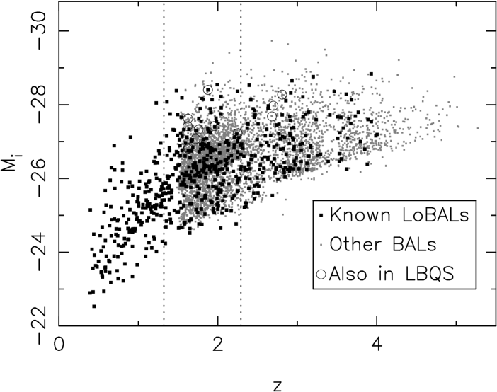
Figure 2: Large, dark squares show the absolute $i$-magnitude and redshift of the LoBALs (with Al III or Mg II $BI_{0}>0$) in this catalog. Smaller, grey squares show the same for HiBALs or sources that did not have low-ionization regions in the SDSS bandpass and could therefore not be classified as HiBALs or LoBALs with certainty (see §1). For the region between the vertical dotted lines, the full Al III and Mg II BAL absorption regions are in the SDSS bandpass. BAL QSOs which are also in the LBQS are circled.

The redshift and absolute $i$-magnitude (obtained from the DR5 catalog) are plotted for our BAL sources in Figure 2. In Table 1, we list the UV spectral properties for all QSOs in the DR5 catalog that show Si IV, C IV, Al III, or Mg II BALs identified by the procedures described in §2. Table 1 contains 5039 QSOs in all, with $BI_{0}>0$ for 1083 BALs attributed to Si IV, 4664 BALs attributed to C IV, 391 BALs attributed to Al III, and 332 BALs attributed to Mg II. For each source with $BI_{0}>0$ for at least one of these ions, we list the name, right ascension (RA), declination (using J2000 coordinates), and redshift given in the DR5 catalog. For each ion (Si IV, C IV, Al III, and Mg II), we list the measurements for $BI$, $BI_{0}$, $EW_{0}$, $v_{min}$, $v_{max}$, and $f_{deep}$ (see below). Although it is, in principle, possible to calculate formal errors for $BI$ and $EW$ measurements, we do not report formal errors in the tables. The true error in these measurements is dominated by the continuum placement and the absorption trough shape, which in turn determines which spectral bins are included in BAL troughs. We therefore do not report formal errors, because they are an inaccurate measure of the complex factors involved.

The quantity $EW_{0}$ is the rest-frame absorption equivalent width measured in BAL regions, i.e., in spectral bins which are part of a continuous absorption region $\geq$10% below the continuum and $>$2000 km s^-1 wide. Narrower absorption troughs are not included in this measurement. We define $v_{max}$ and $v_{min}$ to be the outflow velocities corresponding to the shortest and longest wavelengths, respectively, in the BAL trough(s) of a given spectrum, where a BAL trough is any region for which the flux drops $\geq$10% below the continuum for a velocity range of $>$2000 km s^-1. For example, if a given spectrum has two C IV BALs extending from –20,000 to –15,000 km s^-1 and from –8000 to –5000 km s^-1, then for this source the C IV $v_{max}=-20,000$ and $v_{min}=-5000$ km s^-1. The quantity $f_{deep}$ is defined to be the fraction of BAL bins that fall at least 50% below the continuum. (The definition of “spectral bin” is given in §2.)

We also report, for each ion, the EmLost and BALManyBadBins flags. For C IV we also report the BlueWingAbs flag. Finally, we report measured values of the monochromatic luminosities $L_{\nu}(1400~{}\mathring{\rm A})$ and $L_{\nu}(2500~{}\mathring{\rm A})$ (corrected for Galactic reddening), as well as $SN_{1700}$, which we use to estimate the S/N associated with the measurement of C IV absorption. $SN_{1700}$ is defined as the median of the flux divided by the noise (reported by the SDSS pipeline) for all spectral bins in the 1650–1750 Å region, using the intrinsic binning provided in the SDSS spectra. This wavelength region was selected to be (typically) free of strong absorption, but still near the C IV BAL region. $SN_{1700}$ depends on many factors, including the integration time and the source redshift and luminosity; we use it simply to construct samples of QSOs that are less influenced by selection effects associated with low S/N.

We have used the same procedures to analyze additional spectra of DR5 QSOs that are available in the DR6 public database. These spectra provide one or more additional epochs of SDSS spectroscopy that can be used to study the variability of BALs on (rest-frame) time scales up to $\approx$1 yr. As previous studies of samples of BAL QSOs have shown, BALs commonly vary significantly on such time scales (e.g. Barlow, 1993; Lundgren et al., 2007; Gibson et al., 2008b). However, we caution that $BI$ measures can change dramatically due to small changes in a few spectral bins and, for this reason, $BI$ and $BI_{0}$ alone are not necessarily good metrics of variability. A full variability study should account for these issues as well as differences in S/N and calibration issues between epochs; such a study is beyond the scope of this work. In Table 2, we report the UV spectral properties measured for each available spectrum of any QSO that has at least one BAL with $BI_{0}>0$ for any epoch. Additionally, we report the MJD, plate, and fiber numbers used to uniquely identify each spectrum. The MJD field is the modified Julian date of each SDSS observation.

In Table 3, we list 118 DR5 QSOs that have the C IV BlueWingAbs flag set, but are not considered to have C IV BALs in this catalog. Because these QSOs have emission features that are not well-matched by a single, symmetric Voigt profile, the absorption in these cases is more difficult to accurately determine. Small (and somewhat subjective) changes to the continuum placement for these QSOs can affect whether or not we measure $BI_{0}>0$ in some cases.

During the visual inspection process, we have identified BAL troughs that are likely associated with ions other than Si IV, C IV, Al III, or Mg II. In particular, Si IV BALs may be contaminated by C II $\lambda$1335 Å, Al III BALs by Si II $\lambda$1808 Å, and Mg II BALs by Fe II absorption at rest wavelengths such as $2750$, $2632$, and $2414$ Å. In Table 4, we list 92 BAL QSOs in our catalog that show visual evidence of probable contamination. In the table, we identify the ion for which BAL contamination is likely.

We have searched the Chandra and XMM-Newton archives for targeted or serendipitous observations of BAL QSOs in this catalog. The data analysis for the X-ray observations is described in §4.6. We report in Table 5 the relevant X-ray properties for the 73 radio-quiet sources at $z<2.68$ described in that section. The redshift cut ensures that the 2500 Å continuum flux can be accurately determined.

4 ANALYSIS AND DISCUSSION

In the following sections, we briefly analyze the absorption and emission properties of BAL QSOs and discuss some physical implications of these properties. Because BALs can appear at a range of velocities, we consider only QSOs at redshifts sufficiently high that the entire velocity range (defined to be –25,000 to 0 km s^-1) is visible in the SDSS spectra. For the various ions we consider, these redshift ranges are: $1.96\leq z\leq 5.55$ (Si IV), $1.68\leq z\leq 4.93$ (C IV), $1.23\leq z\leq 3.93$ (Al III), and $0.48\leq z\leq 2.28$ (Mg II). Catalog users who wish to conduct statistical studies of BAL properties should, in most cases, apply similar redshift criteria when selecting their samples to ensure that additional BAL absorption is not missed because it falls outside the SDSS spectral bandpass. Similar bandpass constraints are necessary when assembling a sample of QSOs that are required to be free of BAL features.

4.1 BAL QSO Reddening

Previous studies have found that BAL QSOs are redder than non-BAL QSOs, with LoBALs even redder than HiBALs (e.g., Weymann et al., 1991; Brotherton et al., 2001; Reichard et al., 2003; Trump et al., 2006). In order to investigate reddening in DR5 BAL QSOs, we measure the ratio of the continuum flux densities (in ergs s^-1 cm^-2 Hz^-1) at 1400 Å and 2500 Å. (The continuum flux densities are calculated from the continuum fit alone with emission lines excluded from the model. The continuum-fitting procedures described in §2 should make continuum placement relatively independent of line emission and/or absorption.) This ratio, $R_{red}\equiv F_{\nu}(1400~{}\mathring{\rm A})/F_{\nu}(2500~{}\mathring{\rm A})$, is plotted in Figure 3 for HiBAL, LoBAL, and non-BAL QSOs at $1.96\leq z\leq 2.28$. The distribution of $R_{red}$ for HiBALs is similar to that of non-BALs, but shifted to lower $R_{red}$. The distribution for LoBALs is much broader and shifted to even lower $R_{red}$.

Lower $R_{red}$ values could be due to increased dust reddening, to a different shape for the underlying continuum emission, or to a combination of both factors. The median value of $R_{red}$ is 0.75 for non-BAL QSOs, 0.64 for HiBAL QSOs, and 0.30 for LoBAL QSOs. If we assume that all QSOs have similar emission continuum slopes and the differences are attributed completely to SMC-like dust reddening, HiBAL QSOs have a typical $E(B-V)\approx 0.023$ and LoBALs have $E(B-V)\approx 0.14$ compared to non-BAL QSOs. The $E(B-V)$ value for HiBALs agrees with that found by Reichard et al. (2003), while the LoBAL reddening is somewhat stronger in our sample than the value of 0.077 reported in that study. The difference between HiBAL and LoBAL reddening is $\Delta E(B-V)\approx 0.117$, similar to the value $E(B-V)\approx 0.1$ found by Sprayberry & Foltz (1992).

4.2 Fraction of BAL QSOs in SDSS

The observed fraction of BAL QSOs in optical surveys differs from the intrinsic fraction due to selection effects (e.g., Hewett et al., 1995; Krolik & Voit, 1998; Reichard et al., 2003; Dai et al., 2008; Knigge et al., 2008). Because BAL QSOs are redder than non-BAL QSOs (§4.1), they are rejected in magnitude-limited surveys at a higher rate than less-reddened QSOs of the same intrinsic luminosity. Furthermore, color-selection criteria may incorrectly classify BAL QSOs due to the influence of absorption on BAL QSO colors. BAL identification is also dependent on the S/N ratio of the spectrum, because bins in the middle of a broad absorption feature can randomly rise above the 90% continuum level and prevent the formal identification of a BAL. At lower S/N, this occurs more frequently. False identifications can also occur when the S/N level is low, due to continuum mis-placement or flux levels randomly falling below the required threshhold for BAL identification.

Figure 4 shows the fraction of QSOs with C IV BALs as a function of $SN_{1700}$. Each point in the plot represents the fraction of BAL QSOs in a bin of 2000 QSOs arranged in order of increasing $SN_{1700}$. The $x$ coordinate of each point represents the center of the bin. The “error bars” represent 1$\sigma$ limits on the fractions calculated using a binomial distribution. We show the observed fractions of cases with $BI>0$ and also for the larger class with $BI_{0}>0$. The observed fraction of cases with $BI_{0}>0$ rises with $SN_{1700}$ to $\approx$15% at higher S/N levels. The difference in BAL fractions may not be attributable to S/N alone, as $SN_{1700}$ is correlated with the observed flux and also the QSO luminosity.

At redshifts $z<2.3$, the SDSS color selection criteria are relatively unaffected by BAL absorption, and the typical level of reddening for BAL QSOs causes them to be $\sim$0.15 to 0.2 mag fainter than non-BAL QSOs (Reichard et al., 2003; Knigge et al., 2008). In order to estimate the intrinsic fraction of BAL QSOs, we have identified all optically-selected QSOs with $SN_{1700}\geq 9$, $i\leq 18.5$, and $1.68\leq z\leq 2.3$. We call this set of QSOs subsample $S_{0}$. The S/N cut minimizes the tendency of BALs to go undetected in low-S/N spectra. The $i$-magnitude cut is brighter than the SDSS limit to allow us to examine BAL QSOs that are fainter than the parent sample due to excess reddening. The lower limit on redshift ensures that the full C IV absorption region is in the SDSS spectral bandpass, and the upper redshift limit represents the point at which SDSS selection effects begin to significantly bias the observed BAL fraction (Reichard et al., 2003). We have additionally required that the QSOs in subsample $S_{0}$ be selected for SDSS spectroscopy purely on optical grounds, in order to remove any bias due to specially targeting radio- or X-ray-bright QSOs.

Of the 3427 QSOs in $S_{0}$, 455 have C IV $BI>0$ and 519 have $BI_{0}>0$. This corresponds to BAL fractions of 13.3% ($\pm 0.6$%) and 15.1% ($\pm 0.6$%), respectively. The stated errors are 1$\sigma$ ranges calculated from the binomial distribution, but do not include additional error due to inaccuracies in the estimates of BAL QSO selection effects in the SDSS.

These numbers do not account for the fact that BAL QSOs tend to be redder than non-BAL QSOs and therefore more likely to be excluded in a flux-limited sample. If we make the assumption that BAL QSOs are drawn from a parent population $\Delta m~{}i$-magnitudes brighter, we can estimate the intrinsic BAL fraction by comparing the number of BAL QSOs with $18.7\geq i\geq 17.7$ to non-BAL QSOs with $18.7-\Delta m\geq i\geq 17.7-\Delta m$. For $\Delta m=0.16$ (corresponding to $E(B-V)=0.023$ at 2500 Å), the intrinsic C IV BAL fractions are 16.4 $\pm 0.6$% ($BI>0$) and 18.5 $\pm 0.7$% ($BI_{0}>0$), respectively. However, because the number of DR5 QSOs per unit magnitude is a rapidly-increasing function of $i$-magnitude, these fractions are highly dependent on the idealized assumption that we can directly compare BAL QSOs to a (presumed) parent population $\Delta m~{}i$-magnitudes brighter. A similar method was used by Hewett & Foltz (2003) to obtain a fraction of 22 $\pm 4$% for the LBQS BAL sample. Our estimated BAL fraction agrees reasonably well with those from surveys of QSOs identified in other wavebands such as the radio (18 $\pm 4$%; Becker et al., 2000) and infrared (20 $\pm 2$%; see §6 of Dai et al., 2008).

It has been previously suggested that more-luminous QSOs are more likely to show BALs in their spectra (Ganguly et al., 2007). In order to test for luminosity dependence of the intrinsic BAL fraction, we have divided subsample $S_{0}$ into two groups depending on whether the monochromatic luminosity at 2500 Å is greater or less than the median value of $1.81\times 10^{31}$ erg s^-1 Hz^-1. We find 231 (264) of 1713 lower-luminosity QSOs have $BI>0$ ($BI_{0}>0$), compared to 224 (255) of 1714 QSOs in the higher-luminosity group. A Kolmogorov-Smirnov test finds no indication of differing distributions of $BI_{0}$ for the higher- and lower-luminosity subsamples. We therefore do not find any significant dependence of the BAL fraction on luminosity in sources with $SN_{1700}\geq 9$. However, we note that the luminosity range of our $S_{0}$ sample is rather small, with $10^{31}\lesssim L_{\nu}(2500~{}\mathring{\rm A})\lesssim 6\times 10^{31}$ erg s^-1 Hz^-1 in most cases, and a larger luminosity baseline is needed to test this result more sensitively. In particular, we note that Brandt et al. (2000) reported (in their §8.1) an observed BAL fraction of only 6 $\pm 2$% for the 87 QSOs at $z<0.5$ in the Bright Quasar Survey (BQS; Schmidt & Green, 1983). These QSOs are generally less luminous than the SDSS QSOs in our sample, suggesting that the BAL fraction may be luminosity-dependent over luminosity ranges wider than that of our SDSS sample.

4.3 Distribution of BI for Si IV and C IV

Figure 5 shows the distributions of $BI_{0}$ for 345 BALs of Si IV (top panel) and 1603 of C IV (bottom panel). In each case, we have considered only QSOs at redshifts sufficiently large that the entire potential absorption region (out to –25,000 km s^-1) is in the SDSS bandpass (§4). The distributions are not strongly affected by spectral S/N, in the sense that a Kolmogorov-Smirnov test finds no significant difference between the distributions of $BI_{0}$ for the full sample and for a high-S/N subsample (scaled and plotted with a dotted line in Figure 5), which has $SN_{1700}>9$.

Stacking BAL spectra in groups ordered by $BI_{0}$ can provide a qualitative picture of trends that distinguish strong BALs from weaker BALs. For illustrative purposes, we have constructed median and mean spectra of BAL QSOs with $SN_{1700}\geq 9$ at a range of $BI_{0}$ values. First, we arranged all BAL spectra with $SN_{1700}\geq 9$ in order of increasing $BI_{0}$. We divided this ordered set of spectra into four groups of equal size (111 per group for Si IV, 400 per group for C IV), so that each group represents a unique range of $BI_{0}$. We divided each individual spectrum by its emission model to construct an absorber “transmission spectrum,” and rebinned these spectra to a common grid. Finally, for each wavelength bin at wavelength $\lambda$ in the grid, we determined the median, $M(\lambda)$, of all the transmission spectra in a given group. Plots of the median and mean spectra $M(\lambda)$ are shown for each group in Figure 6 (for Si IV BALs) and Figure 7 (for C IV BALs).

Two local maxima seen at $\approx$1305 Å and $\approx$1335 Å in the median spectra for Si IV BALs (Figure 6) are likely due to unmodeled emission from lines such as O I $\lambda$1306 and C II $\lambda$1335. Apart from the effects of unmodeled emission, the median spectra for Si IV and C IV BALs are qualitatively similar. The broad, shallow features in the median spectra for the low-$BI_{0}$ groups reflect a tendency for weaker BALs to appear at a wide range of velocities. Stronger BAL absorption tends to appear at lower outflow velocities.

4.4 Distribution of $v_{max}$ and $v_{min}$

Figure 8 shows the distribution of $v_{max}$ and $v_{min}$ values for 344 Si IV and 1603 C IV BALs with $SN_{1700}\geq 9$ and $BI_{0}>0$. The distribution for Si IV drops at outflow velocities of about –15,000 and –20,000 km s^-1. These drops are attributable to BAL troughs that would otherwise terminate near these velocities being filled in by the emission features mentioned in §4.3. We also show the distribution of $|v_{max}-v_{min}|$ for the same BALs in Figure 9. Note that, by definition (§3), the velocity range between $v_{max}$ and $v_{min}$ may include relatively unabsorbed regions in cases with multiple BAL troughs for a single ion. Although BAL absorption can cover a wide velocity range, narrower troughs ($<$5000 km s^-1) are more common.

Previous studies have found that BAL maximum outflow velocities are correlated with QSO UV luminosities, as might be expected if BAL outflows are accelerated by radiation pressure (Laor & Brandt, 2002; Ganguly et al., 2007). In order to test this conclusion, we have taken the set of 1239 QSOs with $1.68\leq z\leq 2.68$, C IV $BI_{0}>0$, and $SN_{1700}\geq 9$, and divided it into two subsamples, depending on whether the monochromatic luminosity at 2500 Å falls above or below the median $L_{\nu}(2500~{}\mathring{\rm A})\approx 1.38\times 10^{31}$ erg s^-1 Hz^-1. The median (mean) value of $L_{\nu}(2500~{}\mathring{\rm A})$ for the higher-luminosity subsample is $2.05\times 10^{31}$ ($2.53\times 10^{31}$) erg s^-1 Hz^-1, and for the lower-luminosity subsample it is $1.06\times 10^{31}$ ($1.04\times 10^{31}$) erg s^-1 Hz^-1.

We have plotted the distributions for $v_{min}$ and $v_{max}$ for the lower- and higher-luminosity samples in Figure 10. While the distribution of $v_{min}$ appears to be unrelated to the source luminosity, the distribution of $v_{max}$ differs significantly (at $>$99.99% confidence) between the lower- and higher-luminosity subsamples. Compared to the lower-luminosity subsample, the higher-luminosity QSOs have fewer BALs with $|v_{max}|<15,000$ km s^-1 and more BALs with $|v_{max}|>15,000$ km s^-1. In fact, a Spearman rank correlation test finds a highly significant correlation (at $>$99.99% confidence) between $L_{\nu}(2500~{}\mathring{\rm A})$ and $v_{max}$ for the full sample. If radiation pressure contributes significantly to accelerating the BAL outflow (e.g., Murray et al., 1995), we would expect to see such trends. As noted in §4.2, the luminosity range covered by our sample is limited; stronger effects may be observable with samples covering a wider range of $L_{2500}$.

We caution that low-S/N sources can have BALs obscured due to statistical noise. This effect could lead to a false trend in which lower-luminosity (lower-S/N) sources have lower values of $v_{max}$ due to obscuration of the higher-velocity region of the BAL. We have applied a simple cut to our sample ($SN_{1700}\geq 9$) to limit the effects of low S/N.

It has previously been observed that BALs associated with different ions can have different absorption profiles (e.g., Voit et al., 1993). Here, we briefly compare Si IV and C IV BAL properties using a large sample of SDSS BAL QSOs. There are 798 QSOs in our catalog that have $BI_{0}>0$ for both Si IV and C IV absorption and are also at high enough redshift ($z>1.96$) so that Si IV absorption could be detected up to $|v_{max}|\approx$25,000 km s^-1. In Figure 11 we plot Si IV $v_{min}$ against C IV $v_{min}$ for sources with $SN_{1700}>9$, and in Figure 12 we do the same for $v_{max}$. From these figures, we see that $v_{min}$ is well correlated between the two ions. This supports the general identification of BAL absorption blueward of 1400 Å with Si IV, rather than extremely high-velocity C IV absorption. Si IV tends (with some exceptions) to have equal or greater values of $|v_{min}|$ than C IV does, and also equal or lesser values of $|v_{max}|$. At outflow velocities $|v|\gtrsim 15,000$ km s^-1, the Si IV BAL trough can be truncated by unmodeled emission (such as C II $\lambda$1335); however, the effect is also seen for cases with lower values of C IV $|v_{max}|$. Additional unmodeled emission may be affecting the Si IV trough even at lower outflow velocities, but strong lines are not typically seen at these wavelengths in AGN spectra, and according to theoretical line lists (e.g., Verner et al., 1996), even stronger line emission would be noticable from the same ions in other spectral regions.

Visual inspection indicates that the narrower Si IV troughs can, in some cases, be attributed to the fact that Si IV troughs are shallower and may be categorized as narrower because their high- and low-velocity regions lie above the 90% continuum line due to a sloping trough shape or spectral noise. If the trough depth is governed by the geometric covering factor, this points to geometric differences between the C IV and Si IV absorbers. For stronger Si IV BALs, differences in outflow velocities also suggest differences in the outflow structure. Studies of individual sources have found that the outflow geometry can differ for ions of various elements (e.g., Arav et al., 1999a, b). Our results for a large sample of BAL QSOs indicate that BAL outflows do, in general, show some ion-dependent structure, if we assume that trough depths are dominated by outflow structure.

We have visually inspected the less-common cases in which the Si IV $|v_{min}|$ is less than that of C IV. In some cases, there is broad absorption at lower velocities for C IV that was not formally detected as a BAL; a less-restrictive measure of identifying broad absorption features would not classify these sources as outliers. In other cases, the BAL troughs are indeed unusual; in particular, we cannot rule out the possibility that extremely high-velocity C IV BALs are being mis-classified as low-velocity Si IV absorption. We have also visually inspected cases where the Si IV $|v_{max}|$ is much larger than that of C IV. The high-velocity absorption attributed to Si IV is typically in the 1330–1340 Å range, and is therefore likely due to contamination by C II $\lambda$1335, as discussed in §2.

4.5 Distribution of C IV Emission

Trump et al. (2006) found that the BAL QSOs in their catalog tended to match emission templates with broader line emission than for non-BAL QSOs, and Richards (2006) has suggested that BAL QSOs may be drawn from a parent sample of QSOs with larger C IV blueshifts and weaker C IV emission. To test the hypothesis that C IV emission is different in BAL QSOs, we constructed two QSO subsamples. For each subsample, we required that $z\geq 1.68$ so that the entire C IV absorption region (out to –25,000 km s^-1) is visible in the SDSS bandpass, and also that $SN_{1700}>9$, in order to ensure that the spectra have high S/N. We also required that the EmLost flag be false for C IV and that $v_{min}$ for any BALs present be $<-10,000$ km s^-1. These samples consist of 369 C IV BAL QSOs and 9597 non-BAL QSOs. While these sources may not, in principle, be completely representative of all BAL QSOs, selecting BALs detached from the C IV emission lines is necessary to ensure that BALs are not noticably affecting C IV line emission. However, we are only using 23% of the available BAL QSO population, and if QSOs having BALs with higher values of $|v_{min}|$ are somehow physically different from the rest of the BAL QSO population, our result will not represent the entire BAL QSO population. We note that Turnshek et al. (1988) identified a small sample of three BAL QSOs having strong, smooth C IV BALs with $v_{min}\approx 0$ km s^-1 and found that they had emission line characteristics differing from those of QSOs with significantly detached BALs. Further study of this subject will clearly be valuable, but is outside the scope of the current work.

Figure 13 shows the distribution of C IV emission equivalent width (EW) for BAL and non-BAL QSOs in our subsamples, while Figure 14 shows the distributions of C IV FWHM. The distribution of EWs is clearly different between the two groups, with BAL QSOs having weaker C IV emission EWs. A Kolmogorov-Smirnov test confirms the difference at $>99.99$% confidence. On the other hand, we find no visual or statistical evidence that the distribution of FWHMs differs. We caution in this case that we have fit line cores and not accounted for (often weakly-constrained) emission features in the red and/or blue wings of the line. If the emission in the line wings or line emission from other ions differs between BALs and non-BALs (e.g., Reichard et al., 2003), we would not be sensitive to these effects.

For non-BAL QSOs, the C IV emission EW is related to the UV luminosity according to the well-known Baldwin effect (Baldwin, 1977), with $\log(EW)\equiv A_{B}+\beta\log(L_{UV})$ and $\beta\approx-0.2$ (e.g., Kinney et al., 1990; Wilhite et al., 2006). If BAL QSOs are derived from a parent population with higher intrinsic UV luminosities than we observe (perhaps because excess UV absorption reddens BAL QSOs; §4.1), and if the Baldwin effect in BAL QSOs is based on the intrinsic (e.g., pre-reddened) luminosity, then the Baldwin effect would lead to weaker emission EWs in BAL QSOs compared to non-BAL QSOs of the same observed UV luminosity.

We have measured the Baldwin effect relation for BAL and non-BAL QSOs separately. To do this, we ordered by $L_{2500}$ the samples of BAL and non-BAL QSOs used to generate Figure 13 and divided them into groups of size 50 (BALs) or 200 (non-BALs). For each group, we record the median $L_{2500}$ and C IV EW. The points in Figure 15 show these values for the sample of BAL QSOs. Fitting these points for the BAL QSOs, we find $A_{B}=7.291\pm 1.40$ and $\beta=-0.188\pm 0.045$; this fit is shown in the figure with a solid line. For non-BAL QSOs, we find $A_{B}=7.830\pm 0.437$ and $\beta=-0.203\pm 0.014$; this fit is shown as a dotted line for comparison. For clarity, we do not plot the non-BAL data points; they are well-represented by the fit line. Both logarithmic slopes are consistent with those previously found for the Baldwin effect, but the normalization for the BAL sample is smaller. Fitting the median EW values reduces the influence of a significant number of outlying sources with extremely weak C IV emission. If we fit directly the EW and $L_{2500}$ values for the full samples, we obtain similar results but with slightly steeper logarithmic slopes of $\beta=-0.24\pm 0.01$ and $\beta=-0.27\pm 0.05$, respectively.

If BAL continuum emission is absorbed compared to non-BAL QSOs, but the C IV emission is unaffected by absorption, we would expect BAL QSOs to have generally larger emission EWs than non-BAL QSOs, contrary to what we observe in Figure 13. If both the line and continuum emission are equally absorbed, the EWs would be unchanged, but continuum luminosities would be fainter. This would shift leftward the trend of EW against $L_{2500}$ plotted in Figure 15. However, a rather large shift is required to explain the discrepancy between BAL and non-BAL fit lines in the figure: $L_{2500}$ would have to change by a factor of $\approx$2. This is much larger than typically observed for BAL QSOs (§4.1, §4.2). While BAL QSOs exhibit a Baldwin effect, it appears that this effect alone does not account for the difference observed between BAL and non-BAL QSO C IV emission EWs.

Since we have only considered BAL QSOs that do not have strong BAL features obscuring the emission line regions, it is not obvious why BAL QSOs should have significantly different C IV emission line properties from non-BAL QSOs. It may be that the BAL absorber or other absorbers associated with the BAL outflow along the line of sight partially obscure the broad emission line region (BELR). The low-velocity absorption profile would have to be broad and smooth so that significant deficits in the line emission profile were not detected as BALs. More complex scenarios may also be constructed to account for the effects of viewing, at different orientation angles, the anisotropic emission line radiation from the disk and the BAL outflow (e.g., Krolik & Voit, 1998). Additional orientation-dependent effects may be introduced as the emission is absorbed and scattered by material (including the BAL outflow itself) in the QSO nucleus.

Alternately, the decreased emission in BAL QSOs could be due to ionization effects. For example, if the ionization state of the emission line region were lower for BAL QSOs than for non-BAL QSOs, perhaps due to the presence of additional absorbing material in BAL QSOs that blocks ionizing photons from the emission line region, then emission from highly-ionized species such as C IV could be inhibited in such cases. In fact, a preliminary analysis of our data indicates that the ratio of C IV to C III] emission EWs is significantly ($>$99.99% confidence) lower for BALs than for non-BAL QSOs, which could indicate that the BELR gas is at a lower ionization state in BAL QSOs. However, this effect could be explained by other factors besides ionization differences between BAL and non-BAL QSOs. Further study is therefore needed to determine the extent and physical implications of any differences between broad line emission in BAL and non-BAL QSOs.

4.6 X-Ray Properties of BAL QSOs

The UV and X-ray luminosities of QSOs are correlated (e.g., Avni & Tananbaum, 1982). Recent studies have carefully quantified the UV/X-ray luminosity relation across $\approx$5 orders of magnitude in UV luminosity (e.g., Strateva et al., 2005; Steffen et al., 2006; Just et al., 2007). This relation is usually expressed in terms of the logarithm of the ratio between the monchromatic luminosities $L_{\nu}$ at 2 keV and 2500 Å with the parameter

$$\alpha_{OX} \equiv 0.3838\log\biggl{(}\frac{L_{\nu}(2~{}\rm{keV})}{L_{\nu}(2500~{}\mathring{\rm A})}\biggr{)}.$$ (2)

For typical QSOs, $\alpha_{OX}$ is a function of $L_{2500}$, the monochromatic luminosity at 2500 Å. Just et al. (2007) found

$$\alpha_{OX}(L_{2500}) = (-0.140\pm 0.007)\log(L_{2500})+(2.705\pm 0.212).$$ (3)

Equation 3 enables quantitative measurement of how the X-ray luminosity of a given QSO differs from that expected for a typical QSO of the same UV luminosity. This difference is parameterized by

$$\Delta\alpha_{OX} \equiv \alpha_{OX}-\alpha_{OX}(L_{2500}),$$ (4)

where $\alpha_{OX}$ is the value observed for a particular source observed to have a UV luminosity of $L_{2500}$, and $\alpha_{OX}(L_{2500})$ is determined for a typical QSO from Equation 3. For example, $\Delta\alpha_{OX}=-0.4$ corresponds to X-ray weakness by a factor of $\approx$11 with respect to typical QSOs of the same UV luminosity, and $\Delta\alpha_{OX}=-0.9$ corresponds to X-ray weakness by a factor of $\approx$220.

Many SDSS QSOs have been observed in targeted or (typically) serendipitous observations with Chandra or XMM-Newton. As part of a study to determine the X-ray properties of non-BAL QSOs, we implemented semi-automated processes to identify such sources and obtain X-ray flux densities from data available in the Chandra and XMM-Newton archives. These procedures are described in detail in Gibson et al. (2008a). Briefly, we determined which SDSS QSOs fell on Chandra ACIS or XMM-Newton MOS/$pn$ chips and reduced these data to obtain source and background spectra in each case. We then used the Cash statistic to fit a broken power law to each unbinned spectrum, with the power law break set at (rest-frame) 2 keV. From this fit, we determined the flux density at 2 keV, $F_{\nu}(2~{}{\rm keV})$. We determined upper and lower limits on $F_{\nu}$ by adjusting the power law norm and re-fitting the remaining spectral parameters until the Cash statistic $C$ changed by $\Delta C=1$.

We used Poisson statistics to determine whether a source was detected (based on expected background count rates) at $>$99% confidence in either the observed-frame full (0.5–8 keV), soft (0.5–2 keV) or hard (2–8 keV) bands. High angular resolution is essential to “resolve away” the X-ray background and maximize the rate of source detections. The excellent resolution and astrometric precision of the Chandra ACIS instrument allowed a high source detection rate even for short exposure times and high off-axis angles. For this reason, in cases where a source was observed multiple times, we selected (in an unbiased way) the longest Chandra ACIS exposure as most representative of source properties. If Chandra ACIS observations were not available, we selected the longest XMM-Newton MOS camera observation to determine X-ray fluxes. We prefer the MOS to the $pn$ camera because the MOS is more effective at “resolving away” the background, resulting in a superior detection fraction for these faint sources.

QSOs with strong radio emission are well known to be relatively X-ray bright (e.g., Worrall et al., 1987; Brinkmann et al., 2000). We wish to identify such sources so that we can understand the emission and absorption processes of BAL QSOs without the added complexity of enhanced X-ray emission that may be associated with a radio jet. For sources observed in the FIRST radio survey (Becker et al., 1995), we obtain the 1.4 GHz core flux densities from the DR5 QSO catalog. For sources that were not covered by the FIRST survey, we used 1.4 GHz flux densities obtained from the NVSS survey (Condon et al., 1998). We estimate the monochromatic luminosity at 5 GHz assuming the radio flux follows a power law with a spectral index $\alpha=-0.8$. We then calculate the radio-loudness parameter (e.g., Sramek & Weedman, 1980; Kellermann et al., 1989),

$$\log(R^{*}) \equiv \log\biggl{(}\frac{L_{\nu}({\rm~{}5~{}GHz})}{L_{2500}}\biggr{)}.$$ (5)

We classify sources with $\log(R^{*})\geq 1$ as “radio-loud” and all other sources as “radio-quiet.” Values of $\log(R^{*})$ (or the upper limit on $\log(R^{*})$) are given in Table 5. In some cases, the radio observations may not be sufficiently sensitive to reach to $\log(R^{*})=1$, but even so these cases are small in number and are not extremely radio-bright (see the discussion in Gibson et al. (2008a). Throughout this section, we only consider radio-quiet sources. A detailed study of the X-ray properties of radio-loud BAL QSOs is being conducted separately (Miller et al., in preparation).

In this work, we consider only sources that are within 10$\arcmin$ of the telescope pointing. At larger off-axis angles, the angular resolution is significantly worse, leading to greater uncertainty in background estimation and a larger fraction of non-detections.

4.6.1 X-Ray Weakness

Compared to typical QSOs of the same UV luminosity, BAL QSOs are unusually X-ray weak (e.g., Green et al., 1995; Brandt et al., 2000) due to strong X-ray absorption (e.g., Green et al., 2001; Gallagher et al., 2001, 2002, and references therein). Figure 16 shows the distribution of $\Delta\alpha_{OX}$ for the 42 radio-quiet HiBAL (top panel) and 8 LoBAL (bottom panel) QSOs in our study. The relatively high fraction of X-ray detections indicates that the X-ray emission of SDSS BAL QSOs is reasonably well-matched to the sensitivities of modern X-ray observatories. As previous studies have indicated (e.g., Gallagher et al., 2006), LoBAL QSOs are found to be significantly X-ray weaker than HiBAL QSOs at 99.99% confidence, according to a Gehan test implemented in the Astronomy Survival Analysis (ASURV) software package (e.g., Isobe & Feigelson, 1990; Lavalley et al., 1992). The extreme X-ray weakness of LoBAL QSOs is presumably due to stronger X-ray absorption.

4.6.2 X-Ray Brightness and BAL Properties

Gallagher et al. (2006) examined the UV and X-ray properties of 35 BAL QSOs with optical/UV spectroscopy in the LBQS. They found that most UV BAL properties were not strongly correlated with X-ray brightness in their sample. The exception was $v_{max}$, which correlated with $\Delta\alpha_{OX}$ at $\approx$99.7% confidence. Motivated by their study, we have tested for correlations between BAL properties and $\Delta\alpha_{OX}$ in our larger sample of DR5 BAL QSOs with Chandra and/or XMM-Newton coverage. We have limited our study to consider only radio-quiet QSOs that are confirmed HiBALs; our results are therefore independent of the effects of enhanced X-ray emission associated with radio jets, any physical factors which may differ between HiBAL and LoBAL QSOs, and also any biases inherent in the Mg II BAL detection process (discussed in §2).

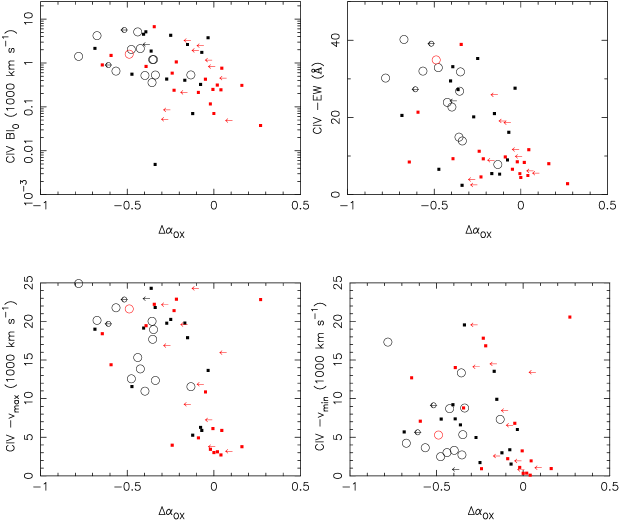
Figure 17: (Top left:) C IV $BI_{0}$ plotted against the relative X-ray brightness $\Delta\alpha_{OX}$ for HiBALs observed in X-rays with Chandra or XMM-Newton. Filled squares represent sources from this catalog that were detected in X-rays, while arrows represent sources from this catalog that were not detected in X-rays. Open circles represent sources from Gallagher et al. (2006) that are not included in this catalog and were detected in X-rays. Smaller circles with arrows represent sources from Gallagher et al. (2006) that are not included in this catalog and were not detected in X-rays. Black points have $L_{2500}\geq 1.44\times 10^{31}$ erg s^-1, while red points have lower values of $L_{2500}$. (Top right:) the same, but plotting C IV BAL absorption EW against $\Delta\alpha_{OX}$. (Bottom left:) the same, but plotting C IV BAL absorption $v_{max}$ against $\Delta\alpha_{OX}$. (Bottom right:) the same, but plotting C IV BAL absorption $v_{min}$ against $\Delta\alpha_{OX}$.

We have plotted the C IV BAL $BI_{0}$, $EW_{0}$, $v_{max}$, and $v_{min}$ against $\Delta\alpha_{OX}$ in Figure 17. In each panel, we have plotted data from this catalog with filled squares for X-ray detected sources, or arrows indicating 1$\sigma$ upper limits, in cases where the source was not detected in X-rays. We have also plotted HiBALs from Gallagher et al. (2006) that were not included in the SDSS DR5 QSO catalog. The Gallagher et al. (2006) non-SDSS HiBALs are plotted with open circles (for detected sources) or circles containing arrows (indicating upper limits for non-detected sources). For these sources, we have measured C IV $BI_{0}$ and $v_{min}$ from the LBQS spectra using the procedures of this catalog. As the figures show, the SDSS BALs extend the range of the Gallagher et al. (2006) study to include weaker BALs at lower maximum outflow velocities, and such sources tend to be less X-ray weak, i.e., they tend to have X-ray luminosities more similar to those of non-BAL QSOs. We have coded the points in Figure 17 so that black points represent sources with higher UV luminosities, having $L_{2500}\geq 1.44\times 10^{31}$ erg s^-1. Red points represent less UV-luminous sources. While the less UV-luminous sources can be found with a wide range of BAL properties, they preferentially have weaker BAL features (i.e., lower values of $BI_{0}$ and $|EW|$) and are not as X-ray weak as the sources with higher values of $L_{2500}$.

Using Kendall’s Tau test as implemented in ASURV, we have tested for correlations between C IV BAL properties and $\Delta\alpha_{OX}$ for the QSOs in this catalog alone, and also for the combined sample with the Gallagher et al. (2006) sources included. In cases where a Gallagher et al. (2006) source was observed in the SDSS, we used the measurements from our current study. The results of our correlation tests are shown in Table 6. We find correlations at $>$95% confidence between $BI_{0}$, $EW_{0}$, $v_{max}$, and $v_{min}$ for HiBALs in our sample alone; with the inclusion of the Gallagher et al. (2006) HiBAL sources, the significance rises to $>99.9$% in some cases. $f_{deep}$ does not show significant evidence for correlation with $\Delta\alpha_{OX}$. While the correlation between $v_{min}$ and $\Delta\alpha_{OX}$ is formally significant at high confidence, Figure 17 suggests that this is primarily due to a lack of high $|v_{min}|$ for relatively X-ray bright sources. As Table 6 shows, we find no significant correlations between BAL properties and the UV luminosity, $L_{\nu}(2500~{}\mathring{\rm A})$, alone. However, we previously observed (in §4.4, using a much larger sample) that BAL QSOs with higher UV luminosities are more likely to have higher $|v_{max}|$ values.

Taken together, these correlations suggest that the X-ray absorber plays an important role in the acceleration of BAL outflows. The depth of a BAL trough is likely determined by the fraction of the UV emission region covered by the BAL outflow at a given velocity (Arav et al., 1999a). This geometry may be relatively independent of the interior X-ray absorber, and thus it is not surprising that $f_{deep}$ is unrelated to $\Delta\alpha_{OX}$. However, the BAL $BI$ and $EW$ are strongly dependent on the BAL width, and the correlations between $BI_{0}$, $EW$, $v_{max}$ and $\Delta\alpha_{OX}$ are reasonable in a scenario where the acceleration of the BAL, and therefore its velocity width, are influenced by the X-ray absorber which shields the BAL outflow from overionization and thereby enables efficient line-driven radiative acceleration.

Recent studies have identified an upper “envelope” to absorber outflow velocities that is dependent on UV luminosity (Laor & Brandt, 2002; Ganguly et al., 2007). This envelope may be interpreted as a terminal velocity that a QSO of a given luminosity can support for a radiatively-driven wind. In Figure 18, we plot the C IV $v_{max}$ and $L_{2500}$ values for 42 QSOs that are known to be HiBALs (at $z\geq 1.68$) that also have X-ray data available, together with the envelope (solid line) derived by Ganguly et al. (2007). We divide our sources into X-ray brighter or X-ray weaker subsamples according to whether their $\Delta\alpha_{OX}$ values fall above or below the median value of $-0.17$ for detected sources. The plot shows that X-ray weaker sources with a range of a factor of $\approx$20 in $L_{2500}$ tend to have higher outflow velocities (as can also be seen from Figure 17) and generally lie closer to the envelope than do X-ray brighter sources. Additional analysis is required to determine the nature of any relation between X-ray properties and BAL terminal velocities, but Figure 18 demonstrates that the X-ray absorption mechanism (assumed to be the cause of X-ray weakness) is important to the process of BAL acceleration.

5 CONCLUSIONS

We have presented a catalog of BAL properties for spectra of 5039 BAL QSOs in the SDSS DR5 QSO catalog and also for spectra of DR5 QSOs obtained in additional epochs that are available in the DR6 public database. We have analyzed the UV absorption properties and also the X-ray properties of radio-quiet BAL QSOs that have been observed in targeted or serendipitous Chandra and/or XMM-Newton observations.

A preliminary analysis of the data in this catalog indicates that:

1. BAL QSOs show stronger UV reddening than non-BAL QSOs (§4.1), in agreement with the findings of previous studies. LoBAL QSOs are even redder than HiBAL QSOs, and also have a broader distribution of $R_{red}$, the ratio of flux densities at 1400 and 2500 Å.

2. Estimates of the intrinsic BAL fraction are complicated by low S/N and survey selection effects. This fraction is $\approx$16.4% for traditional BALs, with some uncertainty due to the assumptions made to determine what fraction of BAL QSOs drop out of magnitude-limited surveys. A preliminary analysis of a sample corrected for S/N and survey selection effects finds no dependence of the BAL fraction or distribution of $BI_{0}$ on UV luminosity for the relatively limited luminosity range in our sample.

3. BAL QSOs with higher UV luminosities are more likely to have a high $|v_{max}|$ than lower-luminosity QSOs (§4.4), as expected for a scenario in which radiation pressure accelerates BAL outflows.

4. While Si IV trough profiles are complicated by unmodeled emission at high velocities, there is some evidence that Si IV BAL troughs tend to appear in a narrower velocity range than those of C IV (§4.4). Because Si IV is found at slightly lower ionization stages than C IV, this trend may reveal ionization-dependent structure in BAL outflows.

5. BAL QSOs and non-BAL SDSS QSOs both follow Baldwin effect relations between C IV emission and UV luminosity with similar logarithmic slopes. However, BAL QSOs tend to have weaker C IV line emission than do non-BAL QSOs (§4.5). This effect may be due to additional, unmodeled absorption of broad emission lines, or to the obstruction of ionizing X-ray photons from the BELR gas.

6. As previous studies have found, radio-quiet HiBAL QSOs are generally relatively X-ray weak compared to non-BAL QSOs, and radio-quiet LoBAL QSOs are even more X-ray weak than HiBAL QSOs are (§4.6.1). The X-ray weakness is attributed to strong X-ray absorption that is necessary to shield the BAL outflow from over-ionization.

7. In general, a larger degree of relative X-ray weakness is associated with stronger C IV BAL absorption and faster outflow velocities in radio-quiet, HiBAL QSOs (§4.6.2). These trends are consistent with a scenario in which strong X-ray absorption enables and enhances the effectiveness of radiation pressure to accelerate the BAL outflow.

In the near future, a web page will be established to track information relevant to this work. Until that time, please contact R. Gibson at the email address at the top of this document. After 2008 December, R. Gibson may be contacted at the University of Washington.

Table 1: DR5 BAL Catalog

DR5 Name	RA	Dec	$z$	Si IV	Si IV	Si IV	Si IV	Si IV	Si IV	C IV	C IV	C IV	C IV
	(J2000)	(J2000)		$BI$ (km s-1)	$BI_{0}$ (km s-1)	$EW_{0}$ (Å)	$v_{min}$ (km s-1)	$v_{max}$ (km s-1)	$f_{deep}$	$BI$ (km s-1)	$BI_{0}$ (km s-1)	$EW_{0}$ (Å)	$v_{min}$ (km s-1)
$000013.80-005446.8$	0.057505	$-0.913004$	1.84	$0$	$276.6$	$-6.2$	$-2249$	$-4872$	$0.58$	$0$	$404.3$	$-9.9$	$-358$
$000038.65+011426.3$	0.161078	$1.240640$	1.84	$1733.2$	$1733.2$	$-15.9$	$-6778$	$-10295$	$0.75$	$2144.7$	$2144.7$	$-19.2$	$-5923$
$000046.41+011420.8$	0.193415	$1.239118$	3.76	$801.3$	$801.3$	$-8.2$	$-7157$	$-10537$	$0.61$	$5803.2$	$5803.2$	$-44.6$	$-4232$
$000051.56+001202.5$	0.214856	$0.200710$	3.88	$1008.6$	$1435.0$	$-12.4$	$-2423$	$-6701$	$0.74$	$2170.4$	$2759.8$	$-22.7$	$-2258$
$000056.89-010409.7$	0.237056	$-1.069386$	2.11	$842.1$	$1504.2$	$-12.5$	$-2214$	$-6700$	$0.65$	$1355.5$	$2353.8$	$-20.7$	$-1497$
$000013.80-005446.8$	$-3326$	$0.77$	$0$	$0$	$0$				$0$	$0$	$0$
$000038.65+011426.3$	$-10544$	$0.85$	$0$	$0$	$0$				$0$	$0$	$0$
$000046.41+011420.8$	$-19529$	$0.78$	$0$	$0$	$0$
$000051.56+001202.5$	$-8054$	$0.86$	$0$	$0$	$0$
$000056.89-010409.7$	$-8605$	$0.56$	$0$	$0$	$0$				$0$	$0$	$0$
$000013.80-005446.8$		1	1	0	0	0	0			1	$3.7$	$-27.55$	$-27.38$
$000038.65+011426.3$		0	0	0	0	0	0			0	$2.9$	$-27.70$	$-27.49$
$000046.41+011420.8$		1	1	0	0	0	0			0	$4.2$	$-27.37$
$000051.56+001202.5$		0	1	0	0	0	0			0	$4.6$	$-27.45$
$000056.89-010409.7$		1	0	0	0	0	0			0	$4.7$	$-27.51$	$-27.15$

Table 2: DR5 BAL Catalog Duplicate Spectra

DR5 Name	RA	Dec	$z$	MJD	Plate	Fiber	Si IV	Si IV	Si IV	Si IV	Si IV	Si IV	C IV
	(J2000)	(J2000)					$BI$ (km s-1)	$BI_{0}$ (km s-1)	$EW_{0}$ (Å)	$v_{min}$(km s-1)	$v_{max}$(km s-1)	$f_{deep}$	$BI$ (km s-1)
$000056.89-010409.7$	0.237056	$-1.069386$	2.11	52203	0685	194	$1233.8$	$1885.3$	$-14.1$	$-2145$	$-8632$	$0.36$	$1238.2$
$001130.55+005550.7$	2.877324	$0.930756$	2.31	52519	0686	603	$259.4$	$259.4$	$-5.0$	$-2955$	$-6612$	$0.17$	$245.2$
$001130.55+005550.7$	2.877324	$0.930756$	2.31	52518	0687	339	$76.6$	$76.6$	$-3.3$	$-4404$	$-6888$	$0.03$	$285.8$
$001438.28-010750.1$	3.659519	$-1.130607$	1.82	52518	0687	249	$0$	$0$	$0$				$571.5$
$001824.95+001525.8$	4.603987	$0.257193$	2.43	51816	0390	386	$1697.3$	$2522.0$	$-18.9$	$-1841$	$-7776$	$0.76$	$4371.1$
$000056.89-010409.7$	$1988.4$	$-19.4$	$-1773$	$-8260$	$0.59$	$0$	$0$	$0$				$0$	$0$
$001130.55+005550.7$	$866.8$	$-11.7$	$-1409$	$-6516$	$0.38$	$0$	$0$	$0$				$0$	$0$
$001130.55+005550.7$	$943.4$	$-12.2$	$-1409$	$-6378$	$0.44$	$0$	$0$	$0$				$0$	$0$
$001438.28-010750.1$	$571.5$	$-10.6$	$-3153$	$-6052$	$0.67$	$0$	$0$	$0$				$0$	$0$
$001824.95+001525.8$	$5849.7$	$-39.2$	$-1538$	$-12162$	$0.82$	$9.7$	$9.7$	$-3.2$	$-3551$	$-5691$	$0.00$	$0$	$0$
$000056.89-010409.7$	$0$				1	1	0	0	0	0			0	4.4
$001130.55+005550.7$	$0$				1	1	0	0	0	0			0	9.5
$001130.55+005550.7$	$943.4$	$0$				1	1	0	0	0	0		0	9.8
$001438.28-010750.1$	$0$				0	1	0	0		0			0	7.0
$001824.95+001525.8$	$0$	$0$				0	0	0	0	0	0	0	0	4.0

Table 3: DR5 Non-BALs with C IV BlueWingAbs Flag Set

DR5 Name	RA	Dec	$z$
$000058.77+003510.5$	0.244895	$0.586257$	1.65
$000124.23-093349.8$	0.350965	$-9.563839$	1.63
$000839.31-005336.8$	2.163799	$-0.893578$	2.62
$002018.74-104851.3$	5.078088	$-10.814263$	1.64
$003554.17-001353.0$	8.975741	$-0.231411$	2.78
$003841.36-004254.4$	9.672349	$-0.715120$	1.55
$004218.71+003237.1$	10.577999	$0.543640$	3.06
$005844.81-003934.1$	14.686740	$-0.659494$	1.60
$011202.98-103616.5$	18.012429	$-10.604590$	2.06
$011705.18+152931.7$	19.271614	$15.492161$	1.85
$011918.15-095239.0$	19.825643	$-9.877519$	1.78
$012802.66+000040.9$	22.011116	$0.011362$	1.87
$020755.76+011159.4$	31.982337	$1.199843$	2.07
$022430.17-004131.1$	36.125713	$-0.691996$	1.67
$022534.09+000347.8$	36.392059	$0.063296$	1.73
$022849.70-004550.4$	37.207116	$-0.764002$	2.54
$025103.47-064719.7$	42.764498	$-6.788819$	1.94
$030311.30+002051.3$	45.797098	$0.347600$	1.76
$030758.75+004259.0$	46.994819	$0.716413$	2.52
$032505.57-003445.5$	51.273226	$-0.579311$	2.50
$034000.92+001944.6$	55.003860	$0.329071$	2.67
$073157.88+365557.8$	112.991170	$36.932735$	2.14
$073453.93+422443.7$	113.724745	$42.412157$	1.90
$074136.49+385847.6$	115.402070	$38.979891$	1.87
$080024.41+160152.5$	120.101736	$16.031277$	1.65
$080937.80+421029.3$	122.407505	$42.174819$	1.67
$081145.52+052435.3$	122.939672	$5.409811$	3.57
$082107.11+360303.5$	125.279636	$36.050996$	1.66
$083314.24+482335.4$	128.309371	$48.393181$	1.60
$084951.46+383548.4$	132.464419	$38.596792$	2.43
$085507.83+061117.3$	133.782626	$6.188150$	3.18
$090351.08+535101.0$	135.962844	$53.850293$	2.86
$090539.53+330923.4$	136.414726	$33.156514$	2.82
$091002.53+422100.5$	137.510549	$42.350159$	2.08
$091053.58+563119.9$	137.723266	$56.522218$	2.36
$091342.48+372603.3$	138.427000	$37.434263$	2.13
$091520.41+041557.4$	138.835061	$4.265964$	1.92
$091545.38+083625.7$	138.939124	$8.607161$	1.61
$091741.60+594557.3$	139.423349	$59.765919$	2.20
$091835.40+051544.6$	139.647508	$5.262410$	1.89
$092316.08+325504.2$	140.817004	$32.917851$	1.64
$092550.48+264920.2$	141.460340	$26.822298$	2.07
$092830.60+101406.9$	142.127503	$10.235262$	2.80
$092940.75+321033.0$	142.419819	$32.175839$	1.78
$093330.53+362736.8$	143.377235	$36.460226$	1.61
$093433.86+565509.6$	143.641090	$56.919338$	1.90
$093753.26+381625.3$	144.471948	$38.273704$	3.19
$095108.76+314705.8$	147.786534	$31.784968$	3.03
$095317.39+281926.2$	148.322488	$28.323965$	1.63
$095722.81+622334.9$	149.345077	$62.393040$	2.25
$095805.67+375029.0$	149.523629	$37.841405$	1.95
$100145.01+511611.7$	150.437550	$51.269942$	1.94
$100247.30+451648.5$	150.697102	$45.280166$	1.63
$100425.66+444406.7$	151.106926	$44.735208$	1.77
$101303.73+434606.3$	153.265570	$43.768418$	2.93
$102259.79+010123.6$	155.749157	$1.023223$	1.56
$103227.63+612853.6$	158.115135	$61.481566$	2.31
$103403.87+380248.4$	158.516153	$38.046790$	3.55
$104157.94+473329.6$	160.491423	$47.558243$	1.64
$104212.55+404122.8$	160.552321	$40.689669$	1.74
$105216.05+485619.1$	163.066878	$48.938658$	2.24
$105332.47+293737.6$	163.385319	$29.627115$	2.08
$105623.71+384155.0$	164.098806	$38.698626$	1.85
$110249.51+013640.6$	165.706317	$1.611299$	1.76
$110312.88+120855.9$	165.803696	$12.148876$	1.58
$112249.43+002047.5$	170.705996	$0.346535$	2.57
$112745.14+633618.4$	171.938114	$63.605118$	1.56
$112813.92+494857.1$	172.058017	$49.815880$	1.55
$112906.44+064809.3$	172.276850	$6.802611$	3.22
$114817.70+135949.8$	177.073777	$13.997174$	1.87
$115701.92+562144.9$	179.258005	$56.362482$	2.17
$120720.58+644842.3$	181.835781	$64.811759$	1.85
$121005.00+125904.3$	182.520873	$12.984554$	1.59
$121538.55+340451.9$	183.910634	$34.081101$	2.20
$122145.26+412525.0$	185.438614	$41.423626$	2.03
$123437.37+062803.7$	188.655710	$6.467713$	2.12
$125215.26+475231.1$	193.063601	$47.875327$	1.61
$130140.58+544907.3$	195.419119	$54.818701$	1.75
$131234.56+011409.7$	198.144034	$1.236055$	2.07
$131936.87+114652.3$	199.903666	$11.781212$	2.23
$132707.05+313838.6$	201.779411	$31.644065$	2.81
$134556.93+612509.6$	206.487213	$61.419352$	1.77
$135249.81-031354.3$	208.207550	$-3.231758$	4.75
$135306.34+113804.7$	208.276448	$11.634643$	1.62
$140030.56+594229.7$	210.127351	$59.708277$	1.92
$141438.04+373357.1$	213.658535	$37.565878$	1.57
$141609.15+502925.5$	214.038133	$50.490434$	1.73
$142342.68+572410.5$	215.927859	$57.402930$	1.66
$142901.69+441358.6$	217.257070	$44.232945$	1.62
$143236.18+234914.4$	218.150757	$23.820679$	2.94
$143911.28+563855.3$	219.797039	$56.648710$	1.64
$144650.53+470814.3$	221.710566	$47.137309$	1.69
$144844.81+494834.8$	222.186714	$49.809694$	2.07
$145432.54+343523.9$	223.635601	$34.589985$	1.61
$145609.59+354908.5$	224.039977	$35.819048$	1.61
$145647.53+533539.5$	224.198044	$53.594306$	1.62
$150220.46+465233.5$	225.585282	$46.875985$	4.26
$150344.91+005026.8$	225.937156	$0.840782$	1.88
$151555.26+605156.0$	228.980261	$60.865565$	1.86
$152500.12+414336.8$	231.250508	$41.726898$	1.89
$152952.38+553346.8$	232.468265	$55.563016$	2.94
$154725.59+534814.5$	236.856625	$53.804052$	1.87
$155218.09+045635.2$	238.075379	$4.943133$	1.57
$160329.14+090218.2$	240.871427	$9.038390$	4.74
$162246.27+290054.1$	245.692808	$29.015031$	2.15
$162802.82+301219.1$	247.011771	$30.205308$	2.44
$163045.20+345924.5$	247.688340	$34.990159$	3.36
$163955.00+310048.6$	249.979187	$31.013525$	1.72
$164207.25+354306.0$	250.530227	$35.718337$	2.33
$164547.63+232824.6$	251.448488	$23.473525$	1.86
$165444.63+384808.6$	253.685981	$38.802401$	1.73
$210255.16-064112.2$	315.729853	$-6.686746$	2.11
$212957.88+100347.2$	322.491177	$10.063128$	3.90
$215002.70+011343.8$	327.511251	$1.228854$	3.27
$220116.75+125636.4$	330.319831	$12.943448$	2.92
$221347.32+001928.4$	333.447208	$0.324570$	2.31
$222339.21+003942.1$	335.913409	$0.661708$	2.96
$235833.49-110532.7$	359.639563	$-11.092431$	1.98

Table 4: BALs with Absorption from Other Ions

DR5 Name	RA	Dec	$z$	Si IV Contam?	Al III Contam?	Mg II Contam?
$031856.62-060037.7$	49.735942	$-6.010475$	1.82	1	1	1
$074554.74+181817.0$	116.478093	$18.304736$	1.84	0	0	1
$074850.39+442439.0$	117.209995	$44.410834$	1.20	1	0	1
$080248.19+551328.9$	120.700793	$55.224706$	2.24	0	0	1
$080401.06+230922.5$	121.004436	$23.156270$	1.84	1	0	1
$080501.77+221409.7$	121.257378	$22.236030$	0.46	1	0	0
$081426.45+364713.5$	123.610221	$36.787098$	0.48	1	0	0
$081547.33+555154.0$	123.947212	$55.865010$	1.44	0	0	1
$083942.11+380526.3$	129.925466	$38.090666$	0.95	0	0	1
$084044.41+363327.8$	130.185078	$36.557738$	1.84	0	0	1
$084526.06+010332.2$	131.358610	$1.058945$	1.89	0	0	1
$084554.24+423003.5$	131.476038	$42.500991$	1.85	1	0	0
$085216.78+233916.8$	133.069948	$23.654686$	0.70	0	0	1
$085910.39+423911.2$	134.793316	$42.653126$	1.25	0	1	1
$090106.43+291128.5$	135.276799	$29.191262$	0.55	1	0	0
$090720.29+365050.1$	136.834576	$36.847253$	0.99	1	1	0
$092221.25+084312.8$	140.588543	$8.720224$	0.77	1	0	1
$093224.48+084008.1$	143.102039	$8.668921$	1.14	1	0	1
$093348.37+313335.2$	143.451569	$31.559805$	1.80	1	0	0
$094347.22+324314.2$	145.946760	$32.720627$	1.09	1	0	0
$101927.36+022521.4$	154.864039	$2.422628$	1.52	0	0	1
$102036.09+602339.0$	155.150382	$60.394179$	1.22	0	0	1
$102216.71+345929.6$	155.569661	$34.991574$	1.84	0	0	1
$102236.23+372241.4$	155.650962	$37.378175$	2.12	0	0	1
$102343.13+553132.3$	155.929735	$55.525657$	1.55	1	0	0
$102413.94+465355.3$	156.058095	$46.898705$	1.31	1	0	0
$103349.80+332812.0$	158.457509	$33.470003$	0.95	0	0	1
$103524.68+452008.4$	158.852840	$45.335676$	2.19	0	1	0
$103958.21+061119.7$	159.992549	$6.188832$	0.44	1	0	0
$112001.68+620459.6$	170.007008	$62.083230$	1.44	0	0	1
$112235.98+042228.2$	170.649927	$4.374512$	3.76	0	1	0
$112526.12+002901.3$	171.358859	$0.483701$	1.14	0	0	1
$112828.31+011337.9$	172.117966	$1.227217$	2.64	0	0	1
$113212.92+010441.3$	173.053845	$1.078150$	3.88	0	0	1
$113424.64+323802.4$	173.602671	$32.634015$	1.32	0	0	1
$113734.06+024159.3$	174.391920	$2.699808$	2.76	1	1	0
$114013.74+624156.3$	175.057256	$62.698984$	1.41	1	0	0
$114225.75+663237.4$	175.607303	$66.543737$	1.18	1	0	0
$115436.60+030006.3$	178.652517	$3.001775$	1.46	0	0	1
$120627.62+002335.3$	181.615115	$0.393165$	2.11	0	0	1
$123549.95+013252.6$	188.958127	$1.547953$	2.55	0	0	1
$123816.38+085146.8$	189.568260	$8.863020$	1.09	0	0	1
$124140.51+012228.4$	190.418794	$1.374580$	1.90	1	1	0
$124452.50+583427.6$	191.218759	$58.574354$	1.65	1	0	0
$125942.80+121312.6$	194.928337	$12.220168$	0.29	0	0	1
$130138.87+023137.4$	195.411975	$2.527074$	2.08	1	0	0
$131010.74-003007.2$	197.544790	$-0.502027$	0.55	1	0	0
$131935.61+152040.6$	199.898379	$15.344636$	0.45	1	0	0
$131957.70+283311.1$	199.990434	$28.553085$	1.40	0	0	1
$132139.86-004151.9$	200.416109	$-0.697774$	0.42	1	0	0
$134026.43+634433.1$	205.110163	$63.742535$	0.53	1	0	0
$134145.12-003631.0$	205.438034	$-0.608638$	0.52	1	0	0
$134417.40+125030.9$	206.072505	$12.841917$	1.42	1	0	0
$134818.03+423205.1$	207.075135	$42.534762$	0.40	1	0	0
$134934.14+245540.1$	207.392268	$24.927807$	1.97	1	0	0
$135246.37+423923.5$	208.193219	$42.656554$	1.40	1	0	0
$135421.82+380327.3$	208.590946	$38.057602$	2.21	1	0	0
$140419.53+342807.5$	211.081378	$34.468771$	1.62	0	1	1
$142010.28+604722.3$	215.042863	$60.789546$	1.92	0	0	1
$142216.85+091524.3$	215.570224	$9.256768$	1.41	1	1	1
$142321.84+063031.7$	215.841033	$6.508812$	1.06	1	0	0
$143015.56+634721.5$	217.564840	$63.789328$	1.97	1	0	0
$143156.30+432556.3$	217.984602	$43.432328$	1.34	1	0	0
$143751.16+530706.8$	219.463185	$53.118575$	0.53	1	0	0
$144002.24+371058.5$	220.009350	$37.182922$	0.40	0	0	1
$144406.69+331345.8$	221.027888	$33.229412$	3.58	1	0	0
$144424.55+013457.0$	221.102292	$1.582513$	1.79	1	0	0
$144800.14+404311.7$	222.000614	$40.719921$	1.82	0	0	1
$144838.74+563919.1$	222.161437	$56.655330$	1.83	0	0	1
$144849.30-013524.1$	222.205440	$-1.590050$	0.93	1	1	1
$145138.28+415401.0$	222.909522	$41.900296$	1.34	1	0	0
$145507.23+571651.8$	223.780126	$57.281080$	2.64	0	0	1
$145729.62+042655.7$	224.373450	$4.448831$	1.20	0	0	1
$150848.80+605551.9$	227.203334	$60.931090$	0.36	0	0	1
$154741.96+444340.0$	236.924871	$44.727790$	1.17	1	0	1
$155359.96+005641.4$	238.499834	$0.944841$	2.31	1	0	0
$155816.71+475645.5$	239.569657	$47.945992$	1.27	1	1	0
$160627.56+445503.2$	241.614869	$44.917573$	1.44	1	0	0
$160744.30+513736.2$	241.934600	$51.626749$	2.21	1	1	0
$161013.07+452850.3$	242.554494	$45.480643$	0.65	1	0	0
$163313.28+352050.8$	248.305352	$35.347462$	2.15	0	0	1
$165008.87+311734.7$	252.536981	$31.292988$	1.96	1	0	0
$170602.51+304424.8$	256.510462	$30.740228$	1.45	1	0	0
$170931.01+630357.2$	257.379217	$63.065902$	1.27	0	0	1
$171701.00+304357.6$	259.254169	$30.732683$	0.55	0	1	1
$172341.08+555340.5$	260.921168	$55.894597$	1.76	1	1	1
$210757.67-062010.6$	316.990293	$-6.336294$	2.23	0	0	1
$222700.62-075356.7$	336.752603	$-7.899091$	1.02	0	0	1
$223841.88+142154.9$	339.674541	$14.365252$	3.06	1	0	0
$224117.74-010218.6$	340.323945	$-1.038511$	1.82	0	0	1
$224207.43-093219.3$	340.530964	$-9.538706$	0.81	1	0	0
$235038.95+133816.3$	357.662311	$13.637877$	1.65	1	0	0

Table 5: X-Ray Source Information

SDSS	ObsId	X-Ray	0.5–2 keV Counts	2–8 keV Counts	X-Ray	$\log(R^{*})$	$\log(L_{\rm 2~{}keV})$	$\alpha_{OX}$	$\Delta\alpha_{OX}$
Source		Exposure (ks)	Source/BG	Source/BG	Detected?
$001130.55+005550.7$	0403760301	25.4	34/12.7	29/10.5	1	$<0.70$	26.33	$-1.94$(0.03)	$-0.25$(0.03)
$002331.21-011045.6$	4079	1.9	2/0.6	2/0.7	0	$<1.32$	$<$26.76	$<$$-1.50$	$<$$0.09$
$003135.56+003421.3$	2101	6.7	32/0.4	10/0.7	1	$<0.75$	26.84	$-1.71$(0.03)	$-0.03$(0.03)
$004527.68+143816.1$	6889	11.4	7/0.2	5/0.7	1	$<0.54$	25.62	$-2.37$(0.06)	$-0.62$(0.06)
$005025.13-005718.3$	4825	13.0	16/1.2	12/2.7	1	$<1.13$	26.31	$-1.81$(0.05)	$-0.17$(0.05)
$005355.15-000309.3$	4830	7.1	18/0.1	10/0.3	1	$<0.56$	26.16	$-1.94$(0.04)	$-0.27$(0.04)
$011227.60-011221.7$	4832	5.9	2/0.1	7/0.3	1	$<0.50$	25.14	$-2.36$(0.08)	$-0.69$(0.08)
$024230.65-000029.6$	344	47.4	12/3.0	20/2.6	1	$<0.92$	24.88	$-2.44$(0.06)	$-0.77$(0.06)
$024304.68+000005.4$	0111200201	39.0	84/14.5	49/10.3	1	$<0.64$	26.72	$-1.75$(0.02)	$-0.08$(0.02)
$030000.57+004828.0$	4145	4.7	1/0.7	0/0.5	0	$<0.12$	$<$24.92	$<$$-2.33$	$<$$-0.70$
$034313.77+010336.9$	5650	7.9	41/0.2	26/0.4	1	$<0.73$	26.58	$-1.85$(0.02)	$-0.16$(0.02)
$073739.96+384413.2$	6888	10.5	8/0.1	4/0.3	1	$<0.10$	25.66	$-2.23$(0.07)	$-0.53$(0.07)
$075627.77+445836.4$	3033	7.0	17/0.8	12/1.5	1	$<0.79$	26.52	$-1.78$(0.04)	$-0.12$(0.04)
$082859.97+500451.3$	0303550901	17.0	81/61.6	98/87.3	1	$<1.15$	26.41	$-1.76$(0.03)	$-0.12$(0.03)
$083104.90+532500.1$	5656	11.6	7/0.8	9/4.5	1	$<0.39$	25.87	$-2.19$(0.07)	$-0.47$(0.07)
$084044.41+363327.8$	817	4.1	0/0.7	8/0.4	1	$0.11$	25.61	$-2.27$(0.06)	$-0.56$(0.06)
$084327.88+361723.2$	532	8.1	5/2.7	6/5.8	0	$<1.38$	$<$26.38	$<$$-1.58$	$<$$-0.01$
$084538.66+342043.6$	818	4.2	40/0.2	12/0.3	1	$<0.13$	26.89	$-1.91$(0.03)	$-0.15$(0.03)
$090904.52-000234.5$	5703	1.3	0/0.1	2/0.1	1	$<1.44$	26.28	$-1.56$(0.12)	$-0.02$(0.12)
$091251.87+591600.7$	3034	9.8	1/0.2	1/0.2	0	$<1.17$	$<$25.55	$<$$-1.91$	$<$$-0.34$
$091400.95+410600.9$	509	9.1	2/2.4	3/3.7	0	$<1.18$	$<$26.14	$<$$-1.78$	$<$$-0.17$
$092011.33+495404.0$	6885	1.5	1/0.0	2/0.1	1	$<0.16$	26.17	$-2.08$(0.10)	$-0.36$(0.10)
$092138.45+301546.9$	0150620101	15.8	7/4.1	13/3.2	1	$<0.60$	25.52	$-2.14$(0.08)	$-0.49$(0.08)
$093514.71+033545.7$	5705	1.8	2/0.0	3/0.1	1	$<0.10$	26.32	$-2.08$(0.08)	$-0.34$(0.08)
$093918.07+355615.0$	0021740101	34.0	8/6.3	7/10.8	0	$<0.79$	$<$26.13	$<$$-1.93$	$<$$-0.27$
$094309.56+481140.5$	0201470101	50.1	8/5.8	7/5.2	0	$<0.91$	$<$25.94	$<$$-1.91$	$<$$-0.28$
$095110.56+393243.9$	0111290101	21.2	11/7.6	9/7.5	0	$<1.23$	$<$26.24	$<$$-1.65$	$<$$-0.08$
$095544.91+410755.0$	5759	40.2	11/0.4	11/0.8	1	$<1.08$	25.07	$-2.20$(0.04)	$-0.59$(0.04)
$095944.47+051158.3$	0204791101	15.3	11/18.8	16/8.1	1	$<0.94$	26.29	$-1.71$(0.04)	$-0.11$(0.04)
$100711.81+053208.9$	6882	1.0	9/0.0	6/0.0	1	$<-0.18$	26.83	$-2.05$(0.06)	$-0.25$(0.06)
$104233.86+010206.2$	4086	1.7	4/0.2	3/0.2	1	$<0.72$	26.73	$-1.74$(0.06)	$-0.07$(0.06)
$104705.07+590728.4$	5028	71.1	40/1.9	175/8.2	1	$<0.64$	24.71	$-1.88$(0.00)	$-0.44$(0.00)
$110637.16+522233.4$	0304071201	8.0	5/3.3	12/2.7	1	$<0.98$	26.02	$-1.86$(0.09)	$-0.24$(0.09)
$114111.61-014306.6$	4146	10.0	12/0.2	11/0.4	1	$<0.42$	25.53	$-2.11$(0.06)	$-0.47$(0.06)
$120522.18+443140.4$	4162	29.7	55/4.1	46/6.1	1	$<0.77$	26.25	$-1.87$(0.03)	$-0.22$(0.03)
$120550.19+020131.5$	5700	2.1	8/0.1	2/0.1	1	$<0.16$	26.83	$-1.92$(0.07)	$-0.17$(0.07)
$120626.17+151335.6$	4834	7.1	3/0.2	1/0.3	1	$<0.68$	25.61	$-2.08$(0.08)	$-0.44$(0.08)
$120924.07+103612.0$	1764	1.2	3/-0.0	0/-0.0	0	$0.15$	$<$25.25	$<$$-1.98$	$<$$-0.43$
$120945.11+454404.6$	0033540601	12.5	5/4.8	8/5.8	0	$<0.71$	$<$26.52	$<$$-1.76$	$<$$-0.11$
$121125.48+151851.5$	2104	4.9	4/0.1	2/0.1	1	$<0.54$	25.95	$-2.08$(0.07)	$-0.39$(0.07)
$121205.30+152005.8$	2104	4.9	21/1.0	5/2.2	1	$<1.20$	27.31	$-1.34$(0.04)	$0.27$(0.04)
$121440.27+142859.1$	2456	4.5	1/0.1	0/0.2	0	$<0.31$	$<$25.45	$<$$-2.28$	$<$$-0.59$
$121930.95+104700.1$	2106	4.6	1/0.2	5/0.2	1	$<0.38$	25.74	$-2.14$(0.07)	$-0.46$(0.07)
$122033.87+334312.0$	2118	3.1	132/0.0	53/0.2	1	$<0.68$	27.59	$-1.30$(0.02)	$0.33$(0.02)
$122637.02+013016.0$	0110990201	28.6	24/6.0	8/6.0	1	$<0.66$	26.10	$-1.88$(0.05)	$-0.25$(0.05)
$122654.39-005430.6$	4060	19.8	42/0.7	10/1.1	1	$<0.68$	26.58	$-1.89$(0.02)	$-0.19$(0.02)
$122708.29+012638.4$	0110990201	28.6	10/4.3	6/3.7	1	$<1.00$	25.66	$-2.01$(0.07)	$-0.39$(0.07)
$122726.90-001003.9$	4865	4.9	0/0.1	4/1.3	0	$<0.86$	$<$26.20	$<$$-1.77$	$<$$-0.16$
$130136.12+000157.9$	4862	4.9	4/0.6	4/0.9	1	$<0.36$	25.97	$-2.10$(0.09)	$-0.41$(0.09)
$133428.06-012349.0$	2110	5.1	3/0.0	3/0.2	1	$0.72$	25.87	$-2.23$(0.07)	$-0.50$(0.07)
$133639.40+514605.2$	0084190201	47.5	22/17.4	13/12.5	0	$<1.03$	$<$26.34	$<$$-1.79$	$<$$-0.15$
$142412.13+054033.6$	5177	3.0	7/0.1	3/0.7	1	$<1.03$	26.61	$-1.61$(0.10)	$-0.01$(0.10)
$142620.30+351712.1$	3619	4.7	15/0.6	6/0.8	1	$<0.77$	26.85	$-1.60$(0.05)	$0.04$(0.05)
$142640.83+332158.7$	4255	5.0	0/0.1	1/0.3	0	$<0.93$	$<$25.74	$<$$-1.91$	$<$$-0.32$
$142652.94+375359.9$	542	8.1	11/0.5	9/1.0	1	$<1.05$	26.00	$-1.83$(0.06)	$-0.23$(0.06)
$143031.78+322145.9$	4279	5.0	20/0.1	6/0.2	1	$<0.96$	27.20	$-1.48$(0.04)	$0.16$(0.04)
$143117.93+364706.0$	4126	3.9	7/0.0	3/1.0	1	$<0.87$	26.68	$-1.70$(0.06)	$-0.05$(0.06)
$143411.23+334015.3$	4236	4.6	10/0.0	4/0.2	1	$<1.09$	26.57	$-1.60$(0.06)	$0.00$(0.06)
$143513.89+484149.3$	0110930401	9.1	22/3.1	12/3.1	1	$<0.91$	26.76	$-1.61$(0.03)	$0.02$(0.03)
$143752.75+042854.5$	5704	1.5	1/0.0	0/0.0	0	$<0.17$	$<$26.18	$<$$-2.12$	$<$$-0.39$
$143853.36+354918.7$	3596	4.6	6/0.1	1/0.2	1	$<0.89$	26.27	$-1.73$(0.06)	$-0.13$(0.06)
$144027.00+032637.9$	4942	23.1	6/5.0	11/2.7	1	$<0.87$	25.14	$-2.30$(0.08)	$-0.64$(0.08)
$144625.48+025548.6$	0203050801	7.9	3/2.2	6/3.4	0	$<0.98$	$<$26.58	$<$$-1.65$	$<$$-0.03$
$144842.45+042403.1$	6886	8.9	7/0.2	10/0.3	1	$<0.08$	25.41	$-2.37$(0.08)	$-0.65$(0.08)
$145002.34+421505.2$	5717	4.3	1/0.0	1/0.7	1	$<0.94$	25.82	$-1.97$(0.13)	$-0.34$(0.13)
$154359.44+535903.2$	822	4.5	61/0.2	18/0.2	1	$<0.21$	27.17	$-1.81$(0.03)	$-0.05$(0.03)
$155259.33+551033.9$	0145450601	9.5	13/7.6	13/11.2	0	$<1.33$	$<$27.04	$<$$-1.44$	$<$$0.17$
$155338.19+551401.9$	0145450601	9.5	16/5.6	14/8.7	1	$<0.76$	26.25	$-1.81$(0.06)	$-0.18$(0.06)
$221511.93-004549.9$	4147	4.6	0/0.1	0/0.3	0	$<-0.17$	$<$24.73	$<$$-2.71$	$<$$-0.96$
$234810.54+010551.3$	861	23.2	65/2.4	15/4.0	1	$<1.13$	26.68	$-1.55$(0.02)	$0.05$(0.02)
$235251.16-001950.4$	2115	5.8	7/0.4	1/1.4	1	$<1.15$	26.41	$-1.70$(0.06)	$-0.09$(0.06)
$235253.51-002850.4$	2115	5.8	0/0.1	0/0.3	0	$<0.68$	$<$24.72	$<$$-2.42$	$<$$-0.78$
$235759.42-000420.5$	0303110801	9.5	8/5.1	6/4.9	0	$<1.42$	$<$26.49	$<$$-1.50$	$<$$0.05$

Table 6: Tests for HiBAL C IV Absorption Correlations with $\Delta\alpha_{OX}$

	Only DR5 HiBALs	With G06 HiBALs
	Confidence	Confidence
$BI_{0}$ vs. $\Delta\alpha_{OX}$	98.91	99.97
$EW$ vs. $\Delta\alpha_{OX}$	96.89	99.99
$v_{max}$ vs. $\Delta\alpha_{OX}$	99.97	$>$99.99
$v_{min}$ vs. $\Delta\alpha_{OX}$	99.50	98.88
$f_{deep}$ vs. $\Delta\alpha_{OX}$	78.93	81.70
$BI_{0}$ vs. $L_{\nu}(2500~{}\mathring{A})$	47.74	24.85
$EW$ vs. $L_{\nu}(2500~{}\mathring{A})$	32.75	2.20
$v_{max}$ vs. $L_{\nu}(2500~{}\mathring{A})$	31.16	54.28
$v_{min}$ vs. $L_{\nu}(2500~{}\mathring{A})$	67.60	67.60
$f_{deep}$ vs. $L_{\nu}(2500~{}\mathring{A})$	6.94	40.55

Figure 1: Examples of C IV absorption regions for BAL QSOs that have the C IV EmLost (top) and BlueWingAbs (bottom) flags set. The $x$-axis shows rest-frame wavelength, while the $y$-axis shows the (unsmoothed) flux density scaled arbitrarily. Our model fit is plotted with a thick line.

Figure 3: The distribution of the ratio $R_{red}\equiv F_{\nu}(1400~{}\mathring{\rm A})/F_{\nu}(2500~{}\mathring{\rm A})$ for QSOs with no BALs (thin solid line), for HiBAL QSOs (thick solid line), and for LoBAL QSOs (thick dotted line). The distributions for the BAL QSOs have been renormalized to match the area under the non-BAL QSO distribution for easy comparison.

Figure 4: The fraction of BALs observed in samples of 2000 QSOs as a function of $SN_{1700}$, the median S/N for spectral bins in the 1650–1700 Å range. Filled circles indicate C IV BALs with $BI_{0}>0$ and open squares indicate C IV BALs with $BI>0$. The error bars represent 1$\sigma$ confidence regions generated using binomial statistics. Note that $SN_{1700}$ is not independent of the source luminosity (§4.2).

Figure 5: (Top panel:) The distribution of $BI_{0}$ for Si IV BALs at $z>1.96$. The solid line shows the distribution for all BALs, while the dotted line shows the distribution for QSOs with $SN_{1700}>9$, scaled to match the area of the full distribution. (Bottom panel:) Same as the top panel, but for C IV BALs at $z>1.68$.

Figure 6: Median (solid line) and mean (dotted line) rest-frame spectra of the absorber transmission for Si IV BALs with $BI_{0}>0$. Spectra with Si IV BALs were sorted by $BI_{0}$ and divided into four groups of 111 objects. Each spectrum was divided by its emission model and rebinned to a common wavelength grid. The spectra for each group are plotted in order of increasing $BI_{0}$. The local maxima at shorter wavelengths are attributable to unmodeled emission lines such as O I $\lambda$1306 and C II $\lambda$1335. Vertical dotted lines mark the wavelengths of these two lines.

Figure 7: Median (solid line) and mean (dotted line) rest-frame spectra of the absorber transmission for C IV BALs with $BI_{0}>0$. Spectra with C IV BALs were sorted by $BI_{0}$ and divided into four groups of 400 objects. Each spectrum was divided by its emission model and rebinned to a common wavelength grid. The spectra for each group are plotted in order of increasing $BI_{0}$.

Figure 8: (Top panel:) The distribution of $v_{max}$ (solid line) and $v_{min}$ (dotted line) for Si IV BALs with $SN_{1700}>9$. (Bottom panel:) Same as top panel, but for C IV.

Figure 9: (Top panel:) The distribution of $|v_{max}-v_{min}|$ for Si IV BALs with $SN_{1700}>9$. (Bottom panel:) Same as top panel, but for C IV.

Figure 10: (Top panel:) The distribution of C IV BAL $v_{min}$ for lower-luminosity (solid line) and higher-luminosity (dotted line) QSOs with $SN_{1700}>9$. (Bottom panel:) Same as top panel, but showing the distribution of $v_{max}$.

Figure 11: Si IV BAL $v_{min}$ plotted against C IV BAL $v_{min}$ for QSOs with $SN_{1700}>9$ and $BI_{0}>0$ for both Si IV and C IV. The solid line indicates where $v_{CIV}=v_{SiIV}$.

Figure 12: Si IV BAL $v_{max}$ plotted against C IV BAL $v_{max}$ for QSOs with $SN_{1700}>9$ and $BI_{0}>0$ for both Si IV and C IV. The solid line indicates where $v_{CIV}=v_{SiIV}$.

Figure 13: C IV $\lambda$1549.5 model emission line EW for BAL QSOs (solid histogram) and non-BAL QSOs (dotted histogram). The BAL distribution has been scaled by a constant for easy comparison. We considered only QSOs with $z\geq 1.68$ and $SN_{1700}>9$ to ensure that the entire C IV absorption region (out to –25,000 km s^-1) was available and that spectra had high S/N. The $x$-axis is logarithmic.

Figure 14: Same as Figure 13, but showing the C IV emission line FWHM.

Figure 15: Filled squares indicate the median $\log(L_{2500})$ and median $\log(CIVEW)$ for luminosity-ordered subsamples of 50 BAL QSOs with C IV $BI_{0}>0$ and $SN_{1700}>9$. The rectangles surrounding the filled squares indicate the range of the central two quartiles in EW. The solid line indicates the best fit to these points. The dotted line indicates a fit to a similarly-constructed set of subsamples of non-BAL QSOs.

Figure 16: (Top panel:) The distribution of $\Delta\alpha_{OX}$ (defined in §4.6) for HiBAL QSOs. Upper limits for sources that were not detected in X-rays are plotted with arrows. The arrows are spaced vertically for visual clarity, but only the $x$-axis value is meaningful as an indication of the upper limit value. Each arrow represents a single source. The vertical dotted line indicates $\Delta\alpha_{OX}=0$ for clarity. (Bottom panel:) Same as top panel, but for LoBAL QSOs.

Figure 18: Plot of C IV $v_{max}$ against $L_{2500}$ for known HiBALs at $z\geq 1.68$. Solid squares represent X-ray detected sources with $\Delta\alpha_{OX}$ above the median $\Delta\alpha_{OX}$ value. Open circles represent X-ray detected sources with $\Delta\alpha_{OX}$ below the median value or undetected sources with upper limits below the median. Crosses represent the remaining undetected sources. The solid curve represents the “envelope” from Figure 7 of Ganguly et al. (2007).

References

- Adelman-McCarthy et al. (2007) Adelman-McCarthy, J. K., Agüeros, M. A., Allam, S. S., Anderson, K. S. J., Anderson, S. F., Annis, J., Bahcall, N. A., Bailer-Jones, C. A. L., Baldry, I. K., Barentine, J. C., Beers, T. C., Belokurov, V., Berlind, A., Bernardi, M., Blanton, M. R., Bochanski, J. J., Boroski, W. N., Bramich, D. M., Brewington, H. J., Brinchmann, J., Brinkmann, J., Brunner, R. J., Budavári, T., Carey, L. N., Carliles, S., Carr, M. A., Castander, F. J., Connolly, A. J., Cool, R. J., Cunha, C. E., Csabai, I., Dalcanton, J. J., Doi, M., Eisenstein, D. J., Evans, M. L., Evans, N. W., Fan, X., Finkbeiner, D. P., Friedman, S. D., Frieman, J. A., Fukugita, M., Gillespie, B., Gilmore, G., Glazebrook, K., Gray, J., Grebel, E. K., Gunn, J. E., de Haas, E., Hall, P. B., Harvanek, M., Hawley, S. L., Hayes, J., Heckman, T. M., Hendry, J. S., Hennessy, G. S., Hindsley, R. B., Hirata, C. M., Hogan, C. J., Hogg, D. W., Holtzman, J. A., Ichikawa, S.-i., Ichikawa, T., Ivezić, Ž., Jester, S., Johnston, D. E., Jorgensen, A. M., Jurić, M., Kauffmann, G., Kent, S. M., Kleinman, S. J., Knapp, G. R., Kniazev, A. Y., Kron, R. G., Krzesinski, J., Kuropatkin, N., Lamb, D. Q., Lampeitl, H., Lee, B. C., Leger, R. F., Lima, M., Lin, H., Long, D. C., Loveday, J., Lupton, R. H., Mandelbaum, R., Margon, B., Martínez-Delgado, D., Matsubara, T., McGehee, P. M., McKay, T. A., Meiksin, A., Munn, J. A., Nakajima, R., Nash, T., Neilsen, Jr., E. H., Newberg, H. J., Nichol, R. C., Nieto-Santisteban, M., Nitta, A., Oyaizu, H., Okamura, S., Ostriker, J. P., Padmanabhan, N., Park, C., Peoples, J. J., Pier, J. R., Pope, A. C., Pourbaix, D., Quinn, T. R., Raddick, M. J., Re Fiorentin, P., Richards, G. T., Richmond, M. W., Rix, H.-W., Rockosi, C. M., Schlegel, D. J., Schneider, D. P., Scranton, R., Seljak, U., Sheldon, E., Shimasaku, K., Silvestri, N. M., Smith, J. A., Smolčić, V., Snedden, S. A., Stebbins, A., Stoughton, C., Strauss, M. A., SubbaRao, M., Suto, Y., Szalay, A. S., Szapudi, I., Szkody, P., Tegmark, M., Thakar, A. R., Tremonti, C. A., Tucker, D. L., Uomoto, A., Vanden Berk, D. E., Vandenberg, J., Vidrih, S., Vogeley, M. S., Voges, W., Vogt, N. P., Weinberg, D. H., West, A. A., White, S. D. M., Wilhite, B., Yanny, B., Yocum, D. R., York, D. G., Zehavi, I., Zibetti, S., & Zucker, D. B. 2007, ApJS, 172, 634
- Arav et al. (1999a) Arav, N., Becker, R. H., Laurent-Muehleisen, S. A., Gregg, M. D., White, R. L., Brotherton, M. S., & de Kool, M. 1999a, ApJ, 524, 566
- Arav et al. (1999b) Arav, N., Korista, K. T., de Kool, M., Junkkarinen, V. T., & Begelman, M. C. 1999b, ApJ, 516, 27
- Avni & Tananbaum (1982) Avni, Y. & Tananbaum, H. 1982, ApJ, 262, L17
- Baldwin (1977) Baldwin, J. A. 1977, ApJ, 214, 679
- Barlow (1993) Barlow, T. A. 1993, PhD thesis, AA(California Univ.)
- Becker et al. (2000) Becker, R. H., White, R. L., Gregg, M. D., Brotherton, M. S., Laurent-Muehleisen, S. A., & Arav, N. 2000, ApJ, 538, 72
- Becker et al. (1995) Becker, R. H., White, R. L., & Helfand, D. J. 1995, ApJ, 450, 559
- Brandt et al. (2000) Brandt, W. N., Laor, A., & Wills, B. J. 2000, ApJ, 528, 637
- Brinkmann et al. (2000) Brinkmann, W., Laurent-Muehleisen, S. A., Voges, W., Siebert, J., Becker, R. H., Brotherton, M. S., White, R. L., & Gregg, M. D. 2000, A&A, 356, 445
- Brotherton et al. (2001) Brotherton, M. S., Tran, H. D., Becker, R. H., Gregg, M. D., Laurent-Muehleisen, S. A., & White, R. L. 2001, ApJ, 546, 775
- Cardelli et al. (1989) Cardelli, J. A., Clayton, G. C., & Mathis, J. S. 1989, ApJ, 345, 245
- Condon et al. (1998) Condon, J. J., Cotton, W. D., Greisen, E. W., Yin, Q. F., Perley, R. A., Taylor, G. B., & Broderick, J. J. 1998, AJ, 115, 1693
- Dai et al. (2008) Dai, X., Shankar, F., & Sivakoff, G. R. 2008, ApJ, 672, 108
- Fukugita et al. (1996) Fukugita, M., Ichikawa, T., Gunn, J. E., Doi, M., Shimasaku, K., & Schneider, D. P. 1996, AJ, 111, 1748
- Gallagher et al. (2002) Gallagher, S. C., Brandt, W. N., Chartas, G., & Garmire, G. P. 2002, ApJ, 567, 37
- Gallagher et al. (2006) Gallagher, S. C., Brandt, W. N., Chartas, G., Priddey, R., Garmire, G. P., & Sambruna, R. M. 2006, ApJ, 644, 709
- Gallagher et al. (2001) Gallagher, S. C., Brandt, W. N., Laor, A., Elvis, M., Mathur, S., Wills, B. J., & Iyomoto, N. 2001, ApJ, 546, 795
- Ganguly et al. (2007) Ganguly, R., Brotherton, M. S., Cales, S., Scoggins, B., Shang, Z., & Vestergaard, M. 2007, ApJ, 665, 990
- Gibson et al. (2008a) Gibson, R. R., Brandt, W. N., & Schneider, D. P. 2008a, ApJ, 685, 773
- Gibson et al. (2008b) Gibson, R. R., Brandt, W. N., Schneider, D. P., & Gallagher, S. C. 2008b, ApJ, 675, 985
- Green et al. (2001) Green, P. J., Aldcroft, T. L., Mathur, S., Wilkes, B. J., & Elvis, M. 2001, ApJ, 558, 109
- Green et al. (1995) Green, P. J., Schartel, N., Anderson, S. F., Hewett, P. C., Foltz, C. B., Brinkmann, W., Fink, H., Truemper, J., & Margon, B. 1995, ApJ, 450, 51
- Gunn et al. (1998) Gunn, J. E., Carr, M., Rockosi, C., Sekiguchi, M., Berry, K., Elms, B., de Haas, E., Ivezić, Ž., Knapp, G., Lupton, R., Pauls, G., Simcoe, R., Hirsch, R., Sanford, D., Wang, S., York, D., Harris, F., Annis, J., Bartozek, L., Boroski, W., Bakken, J., Haldeman, M., Kent, S., Holm, S., Holmgren, D., Petravick, D., Prosapio, A., Rechenmacher, R., Doi, M., Fukugita, M., Shimasaku, K., Okada, N., Hull, C., Siegmund, W., Mannery, E., Blouke, M., Heidtman, D., Schneider, D., Lucinio, R., & Brinkman, J. 1998, AJ, 116, 3040
- Gunn et al. (2006) Gunn, J. E., Siegmund, W. A., Mannery, E. J., Owen, R. E., Hull, C. L., Leger, R. F., Carey, L. N., Knapp, G. R., York, D. G., Boroski, W. N., Kent, S. M., Lupton, R. H., Rockosi, C. M., Evans, M. L., Waddell, P., Anderson, J. E., Annis, J., Barentine, J. C., Bartoszek, L. M., Bastian, S., Bracker, S. B., Brewington, H. J., Briegel, C. I., Brinkmann, J., Brown, Y. J., Carr, M. A., Czarapata, P. C., Drennan, C. C., Dombeck, T., Federwitz, G. R., Gillespie, B. A., Gonzales, C., Hansen, S. U., Harvanek, M., Hayes, J., Jordan, W., Kinney, E., Klaene, M., Kleinman, S. J., Kron, R. G., Kresinski, J., Lee, G., Limmongkol, S., Lindenmeyer, C. W., Long, D. C., Loomis, C. L., McGehee, P. M., Mantsch, P. M., Neilsen, Jr., E. H., Neswold, R. M., Newman, P. R., Nitta, A., Peoples, J. J., Pier, J. R., Prieto, P. S., Prosapio, A., Rivetta, C., Schneider, D. P., Snedden, S., & Wang, S.-i. 2006, AJ, 131, 2332
- Hall et al. (2002) Hall, P. B., Anderson, S. F., Strauss, M. A., York, D. G., Richards, G. T., Fan, X., Knapp, G. R., Schneider, D. P., Vanden Berk, D. E., Geballe, T. R., Bauer, A. E., Becker, R. H., Davis, M., Rix, H.-W., Nichol, R. C., Bahcall, N. A., Brinkmann, J., Brunner, R., Connolly, A. J., Csabai, I., Doi, M., Fukugita, M., Gunn, J. E., Haiman, Z., Harvanek, M., Heckman, T. M., Hennessy, G. S., Inada, N., Ivezić, Ž., Johnston, D., Kleinman, S., Krolik, J. H., Krzesinski, J., Kunszt, P. Z., Lamb, D. Q., Long, D. C., Lupton, R. H., Miknaitis, G., Munn, J. A., Narayanan, V. K., Neilsen, E., Newman, P. R., Nitta, A., Okamura, S., Pentericci, L., Pier, J. R., Schlegel, D. J., Snedden, S., Szalay, A. S., Thakar, A. R., Tsvetanov, Z., White, R. L., & Zheng, W. 2002, ApJS, 141, 267
- Hewett & Foltz (2003) Hewett, P. C. & Foltz, C. B. 2003, AJ, 125, 1784
- Hewett et al. (1995) Hewett, P. C., Foltz, C. B., & Chaffee, F. H. 1995, AJ, 109, 1498
- Houck & Denicola (2000) Houck, J. C. & Denicola, L. A. 2000, in ASP Conf. Ser. 216: Astronomical Data Analysis Software and Systems IX, ed. N. Manset, C. Veillet, & D. Crabtree, 591–+
- Isobe & Feigelson (1990) Isobe, T. & Feigelson, E. D. 1990, in Bulletin of the American Astronomical Society, Vol. 22, Bulletin of the American Astronomical Society, 917–918
- Ivezić et al. (2004) Ivezić, Ž., Lupton, R. H., Schlegel, D., Boroski, B., Adelman-McCarthy, J., Yanny, B., Kent, S., Stoughton, C., Finkbeiner, D., Padmanabhan, N., Rockosi, C. M., Gunn, J. E., Knapp, G. R., Strauss, M. A., Richards, G. T., Eisenstein, D., Nicinski, T., Kleinman, S. J., Krzesinski, J., Newman, P. R., Snedden, S., Thakar, A. R., Szalay, A., Munn, J. A., Smith, J. A., Tucker, D., & Lee, B. C. 2004, Astronomische Nachrichten, 325, 583
- Just et al. (2007) Just, D. W., Brandt, W. N., Shemmer, O., Steffen, A. T., Schneider, D. P., Chartas, G., & Garmire, G. P. 2007, ApJ, 665, 1004
- Kellermann et al. (1989) Kellermann, K. I., Sramek, R., Schmidt, M., Shaffer, D. B., & Green, R. 1989, AJ, 98, 1195
- Kinney et al. (1990) Kinney, A. L., Rivolo, A. R., & Koratkar, A. P. 1990, ApJ, 357, 338
- Knigge et al. (2008) Knigge, C., Scaringi, S., Goad, M. R., & Cottis, C. E. 2008, ArXiv e-prints, 802
- Krolik & Voit (1998) Krolik, J. H. & Voit, G. M. 1998, ApJ, 497, L5+
- Laor & Brandt (2002) Laor, A. & Brandt, W. N. 2002, ApJ, 569, 641
- Lavalley et al. (1992) Lavalley, M., Isobe, T., & Feigelson, E. 1992, in ASP Conf. Ser. 25: Astronomical Data Analysis Software and Systems I, ed. D. M. Worrall, C. Biemesderfer, & J. Barnes, 245–+
- Lundgren et al. (2007) Lundgren, B. F., Wilhite, B. C., Brunner, R. J., Hall, P. B., Schneider, D. P., York, D. G., Vanden Berk, D. E., & Brinkmann, J. 2007, ApJ, 656, 73
- Lupton et al. (1999) Lupton, R. H., Gunn, J. E., & Szalay, A. S. 1999, AJ, 118, 1406
- Murray et al. (1995) Murray, N., Chiang, J., Grossman, S. A., & Voit, G. M. 1995, ApJ, 451, 498
- O’Donnell (1994) O’Donnell, J. E. 1994, ApJ, 422, 158
- Pei (1992) Pei, Y. C. 1992, ApJ, 395, 130
- Pier et al. (2003) Pier, J. R., Munn, J. A., Hindsley, R. B., Hennessy, G. S., Kent, S. M., Lupton, R. H., & Ivezić, Ž. 2003, AJ, 125, 1559
- Reichard et al. (2003) Reichard, T. A., Richards, G. T., Hall, P. B., Schneider, D. P., Vanden Berk, D. E., Fan, X., York, D. G., Knapp, G. R., & Brinkmann, J. 2003, AJ, 126, 2594
- Richards (2006) Richards, G. T. 2006, ArXiv Astrophysics e-prints
- Richards et al. (2002) Richards, G. T., Fan, X., Newberg, H. J., Strauss, M. A., Vanden Berk, D. E., Schneider, D. P., Yanny, B., Boucher, A., Burles, S., Frieman, J. A., Gunn, J. E., Hall, P. B., Ivezić, Ž., Kent, S., Loveday, J., Lupton, R. H., Rockosi, C. M., Schlegel, D. J., Stoughton, C., SubbaRao, M., & York, D. G. 2002, AJ, 123, 2945
- Schlegel et al. (1998) Schlegel, D. J., Finkbeiner, D. P., & Davis, M. 1998, ApJ, 500, 525
- Schmidt & Green (1983) Schmidt, M. & Green, R. F. 1983, ApJ, 269, 352
- Schneider et al. (2007) Schneider, D. P., Hall, P. B., Richards, G. T., Strauss, M. A., Vanden Berk, D. E., Anderson, S. F., Brandt, W. N., Fan, X., Jester, S., Gray, J., Gunn, J. E., SubbaRao, M. U., Thakar, A. R., Stoughton, C., Szalay, A. S., Yanny, B., York, D. G., Bahcall, N. A., Barentine, J., Blanton, M. R., Brewington, H., Brinkmann, J., Brunner, R. J., Castander, F. J., Csabai, I., Frieman, J. A., Fukugita, M., Harvanek, M., Hogg, D. W., Ivezić, Ž., Kent, S. M., Kleinman, S. J., Knapp, G. R., Kron, R. G., Krzesiński, J., Long, D. C., Lupton, R. H., Nitta, A., Pier, J. R., Saxe, D. H., Shen, Y., Snedden, S. A., Weinberg, D. H., & Wu, J. 2007, AJ, 134, 102
- Schneider et al. (2005) Schneider, D. P., Hall, P. B., Richards, G. T., Vanden Berk, D. E., Anderson, S. F., Fan, X., Jester, S., Stoughton, C., Strauss, M. A., SubbaRao, M., Brandt, W. N., Gunn, J. E., Yanny, B., Bahcall, N. A., Barentine, J. C., Blanton, M. R., Boroski, W. N., Brewington, H. J., Brinkmann, J., Brunner, R., Csabai, I., Doi, M., Eisenstein, D. J., Frieman, J. A., Fukugita, M., Gray, J., Harvanek, M., Heckman, T. M., Ivezić, Ž., Kent, S., Kleinman, S. J., Knapp, G. R., Kron, R. G., Krzesinski, J., Long, D. C., Loveday, J., Lupton, R. H., Margon, B., Munn, J. A., Neilsen, E. H., Newberg, H. J., Newman, P. R., Nichol, R. C., Nitta, A., Pier, J. R., Rockosi, C. M., Saxe, D. H., Schlegel, D. J., Snedden, S. A., Szalay, A. S., Thakar, A. R., Uomoto, A., Voges, W., & York, D. G. 2005, AJ, 130, 367
- Smith et al. (2002) Smith, J. A., Tucker, D. L., Kent, S., Richmond, M. W., Fukugita, M., Ichikawa, T., Ichikawa, S.-i., Jorgensen, A. M., Uomoto, A., Gunn, J. E., Hamabe, M., Watanabe, M., Tolea, A., Henden, A., Annis, J., Pier, J. R., McKay, T. A., Brinkmann, J., Chen, B., Holtzman, J., Shimasaku, K., & York, D. G. 2002, AJ, 123, 2121
- Sprayberry & Foltz (1992) Sprayberry, D. & Foltz, C. B. 1992, ApJ, 390, 39
- Sramek & Weedman (1980) Sramek, R. A. & Weedman, D. W. 1980, ApJ, 238, 435
- Steffen et al. (2006) Steffen, A. T., Strateva, I., Brandt, W. N., Alexander, D. M., Koekemoer, A. M., Lehmer, B. D., Schneider, D. P., & Vignali, C. 2006, AJ, 131, 2826
- Stoughton et al. (2002) Stoughton, C., Lupton, R. H., Bernardi, M., Blanton, M. R., Burles, S., Castander, F. J., Connolly, A. J., Eisenstein, D. J., Frieman, J. A., Hennessy, G. S., Hindsley, R. B., Ivezić, Ž., Kent, S., Kunszt, P. Z., Lee, B. C., Meiksin, A., Munn, J. A., Newberg, H. J., Nichol, R. C., Nicinski, T., Pier, J. R., Richards, G. T., Richmond, M. W., Schlegel, D. J., Smith, J. A., Strauss, M. A., SubbaRao, M., Szalay, A. S., Thakar, A. R., Tucker, D. L., Vanden Berk, D. E., Yanny, B., Adelman, J. K., Anderson, Jr., J. E., Anderson, S. F., Annis, J., Bahcall, N. A., Bakken, J. A., Bartelmann, M., Bastian, S., Bauer, A., Berman, E., Böhringer, H., Boroski, W. N., Bracker, S., Briegel, C., Briggs, J. W., Brinkmann, J., Brunner, R., Carey, L., Carr, M. A., Chen, B., Christian, D., Colestock, P. L., Crocker, J. H., Csabai, I., Czarapata, P. C., Dalcanton, J., Davidsen, A. F., Davis, J. E., Dehnen, W., Dodelson, S., Doi, M., Dombeck, T., Donahue, M., Ellman, N., Elms, B. R., Evans, M. L., Eyer, L., Fan, X., Federwitz, G. R., Friedman, S., Fukugita, M., Gal, R., Gillespie, B., Glazebrook, K., Gray, J., Grebel, E. K., Greenawalt, B., Greene, G., Gunn, J. E., de Haas, E., Haiman, Z., Haldeman, M., Hall, P. B., Hamabe, M., Hansen, B., Harris, F. H., Harris, H., Harvanek, M., Hawley, S. L., Hayes, J. J. E., Heckman, T. M., Helmi, A., Henden, A., Hogan, C. J., Hogg, D. W., Holmgren, D. J., Holtzman, J., Huang, C.-H., Hull, C., Ichikawa, S.-I., Ichikawa, T., Johnston, D. E., Kauffmann, G., Kim, R. S. J., Kimball, T., Kinney, E., Klaene, M., Kleinman, S. J., Klypin, A., Knapp, G. R., Korienek, J., Krolik, J., Kron, R. G., Krzesiński, J., Lamb, D. Q., Leger, R. F., Limmongkol, S., Lindenmeyer, C., Long, D. C., Loomis, C., Loveday, J., MacKinnon, B., Mannery, E. J., Mantsch, P. M., Margon, B., McGehee, P., McKay, T. A., McLean, B., Menou, K., Merelli, A., Mo, H. J., Monet, D. G., Nakamura, O., Narayanan, V. K., Nash, T., Neilsen, Jr., E. H., Newman, P. R., Nitta, A., Odenkirchen, M., Okada, N., Okamura, S., Ostriker, J. P., Owen, R., Pauls, A. G., Peoples, J., Peterson, R. S., Petravick, D., Pope, A., Pordes, R., Postman, M., Prosapio, A., Quinn, T. R., Rechenmacher, R., Rivetta, C. H., Rix, H.-W., Rockosi, C. M., Rosner, R., Ruthmansdorfer, K., Sandford, D., Schneider, D. P., Scranton, R., Sekiguchi, M., Sergey, G., Sheth, R., Shimasaku, K., Smee, S., Snedden, S. A., Stebbins, A., Stubbs, C., Szapudi, I., Szkody, P., Szokoly, G. P., Tabachnik, S., Tsvetanov, Z., Uomoto, A., Vogeley, M. S., Voges, W., Waddell, P., Walterbos, R., Wang, S.-i., Watanabe, M., Weinberg, D. H., White, R. L., White, S. D. M., Wilhite, B., Wolfe, D., Yasuda, N., York, D. G., Zehavi, I., & Zheng, W. 2002, AJ, 123, 485
- Strateva et al. (2005) Strateva, I. V., Brandt, W. N., Schneider, D. P., Vanden Berk, D. G., & Vignali, C. 2005, AJ, 130, 387
- Tolea et al. (2002) Tolea, A., Krolik, J. H., & Tsvetanov, Z. 2002, ApJ, 578, L31
- Trump et al. (2006) Trump, J. R., Hall, P. B., Reichard, T. A., Richards, G. T., Schneider, D. P., Vanden Berk, D. E., Knapp, G. R., Anderson, S. F., Fan, X., Brinkman, J., Kleinman, S. J., & Nitta, A. 2006, ApJS, 165, 1
- Turnshek et al. (1988) Turnshek, D. A., Grillmair, C. J., Foltz, C. B., & Weymann, R. J. 1988, ApJ, 325, 651
- Vanden Berk et al. (2001) Vanden Berk, D. E., Richards, G. T., Bauer, A., Strauss, M. A., Schneider, D. P., Heckman, T. M., York, D. G., Hall, P. B., Fan, X., Knapp, G. R., Anderson, S. F., Annis, J., Bahcall, N. A., Bernardi, M., Briggs, J. W., Brinkmann, J., Brunner, R., Burles, S., Carey, L., Castander, F. J., Connolly, A. J., Crocker, J. H., Csabai, I., Doi, M., Finkbeiner, D., Friedman, S., Frieman, J. A., Fukugita, M., Gunn, J. E., Hennessy, G. S., Ivezić, Ž., Kent, S., Kunszt, P. Z., Lamb, D. Q., Leger, R. F., Long, D. C., Loveday, J., Lupton, R. H., Meiksin, A., Merelli, A., Munn, J. A., Newberg, H. J., Newcomb, M., Nichol, R. C., Owen, R., Pier, J. R., Pope, A., Rockosi, C. M., Schlegel, D. J., Siegmund, W. A., Smee, S., Snir, Y., Stoughton, C., Stubbs, C., SubbaRao, M., Szalay, A. S., Szokoly, G. P., Tremonti, C., Uomoto, A., Waddell, P., Yanny, B., & Zheng, W. 2001, AJ, 122, 549
- Verner et al. (1995) Verner, D. A., Ferland, G. J., Korista, K. T., & Yakovlev, D. G. 1995, Bulletin of the American Astronomical Society, 27, 859
- Verner et al. (1996) Verner, D. A., Verner, E. M., & Ferland, G. J. 1996, Atomic Data and Nuclear Data Tables, 64, 1
- Voit et al. (1993) Voit, G. M., Weymann, R. J., & Korista, K. T. 1993, ApJ, 413, 95
- Weymann et al. (1991) Weymann, R. J., Morris, S. L., Foltz, C. B., & Hewett, P. C. 1991, ApJ, 373, 23
- Wilhite et al. (2006) Wilhite, B. C., Vanden Berk, D. E., Brunner, R. J., & Brinkmann, J. V. 2006, ApJ, 641, 78
- Worrall et al. (1987) Worrall, D. M., Tananbaum, H., Giommi, P., & Zamorani, G. 1987, ApJ, 313, 596
- York et al. (2000) York, D. G., Adelman, J., Anderson, Jr., J. E., Anderson, S. F., Annis, J., Bahcall, N. A., Bakken, J. A., Barkhouser, R., Bastian, S., Berman, E., Boroski, W. N., Bracker, S., Briegel, C., Briggs, J. W., Brinkmann, J., Brunner, R., Burles, S., Carey, L., Carr, M. A., Castander, F. J., Chen, B., Colestock, P. L., Connolly, A. J., Crocker, J. H., Csabai, I., Czarapata, P. C., Davis, J. E., Doi, M., Dombeck, T., Eisenstein, D., Ellman, N., Elms, B. R., Evans, M. L., Fan, X., Federwitz, G. R., Fiscelli, L., Friedman, S., Frieman, J. A., Fukugita, M., Gillespie, B., Gunn, J. E., Gurbani, V. K., de Haas, E., Haldeman, M., Harris, F. H., Hayes, J., Heckman, T. M., Hennessy, G. S., Hindsley, R. B., Holm, S., Holmgren, D. J., Huang, C.-h., Hull, C., Husby, D., Ichikawa, S.-I., Ichikawa, T., Ivezić, Ž., Kent, S., Kim, R. S. J., Kinney, E., Klaene, M., Kleinman, A. N., Kleinman, S., Knapp, G. R., Korienek, J., Kron, R. G., Kunszt, P. Z., Lamb, D. Q., Lee, B., Leger, R. F., Limmongkol, S., Lindenmeyer, C., Long, D. C., Loomis, C., Loveday, J., Lucinio, R., Lupton, R. H., MacKinnon, B., Mannery, E. J., Mantsch, P. M., Margon, B., McGehee, P., McKay, T. A., Meiksin, A., Merelli, A., Monet, D. G., Munn, J. A., Narayanan, V. K., Nash, T., Neilsen, E., Neswold, R., Newberg, H. J., Nichol, R. C., Nicinski, T., Nonino, M., Okada, N., Okamura, S., Ostriker, J. P., Owen, R., Pauls, A. G., Peoples, J., Peterson, R. L., Petravick, D., Pier, J. R., Pope, A., Pordes, R., Prosapio, A., Rechenmacher, R., Quinn, T. R., Richards, G. T., Richmond, M. W., Rivetta, C. H., Rockosi, C. M., Ruthmansdorfer, K., Sandford, D., Schlegel, D. J., Schneider, D. P., Sekiguchi, M., Sergey, G., Shimasaku, K., Siegmund, W. A., Smee, S., Smith, J. A., Snedden, S., Stone, R., Stoughton, C., Strauss, M. A., Stubbs, C., SubbaRao, M., Szalay, A. S., Szapudi, I., Szokoly, G. P., Thakar, A. R., Tremonti, C., Tucker, D. L., Uomoto, A., Vanden Berk, D., Vogeley, M. S., Waddell, P., Wang, S.-i., Watanabe, M., Weinberg, D. H., Yanny, B., & Yasuda, N. 2000, AJ, 120, 1579