The prospects for a new search for the electron electric dipole moment in solid Gadolinium iron garnet ceramics

Abstract

We address a number of issues regarding solid state electron electric dipole moment (EDM) experiments, focusing on gadolinium iron garnet (abbreviated GdIG, chemical formula Gd₃Fe₅O₁₂) as a possible sample material. GdIG maintains its high magnetic susceptibility down to 4.2 K, which enhances the EDM-induced magnetization of a sample placed in an electric field. We estimate that lattice polarizability gives rise to an EDM enhancement factor of approximately 20. We also calculate the effect of the demagnetizing field for various sample geometries and permeabilities. Measurements of intrinsic GdIG magnetization noise are presented, and the fluctuation-dissipation theorem is used to compare our data with the measurements of the imaginary part of GdIG permeability at 4.2 K, showing good agreement above frequencies of a few hertz. We also observe how the demagnetizing field suppresses the noise-induced magnetic flux, confirming our calculations. The statistical sensitivity of an EDM search based on a solid GdIG sample is estimated to be on the same level as the present experimental limit. Such a measurement would be valuable, given the completely different methods and systematics involved. The most significant systematics in such an experiment are the magnetic hysteresis and the magneto-electric effect. Our analysis shows that it should be possible to control these at the level of statistical sensitivity.

I Introduction

One of the ways to test the Standard Model in low-energy experiments is to search for parity and time-reversal-violating permanent electric dipole moments of particles such as the electron and the neutron. It is well-known that the observed matter-antimatter asymmetry of the Universe can not be explained by the CP-violation mechanisms within the Standard Model Balazs et al. (2005). A variety of theories suggesting new sources of CP-violation exist, many of them are already constrained by the current experimental limit on the electron EDM: $d_{e}<1.6\times 10^{-27}\mbox{ e$\cdot$cm}$ Regan et al. (2002). A number of experimental EDM searches are currently under way, or being developed, they involve diatomic molecules Hudson et al. (2002); Kawall et al. (2004, 2005), molecular ions Stutz and Cornell (2004), cold atoms Weiss et al. (2003), liquids Ledbetter et al. (2005), and solid-state systems Bouchard et al. (2008).

Following the original suggestion of Shapiro Shapiro (1968), we have been investigating the possibility of an improved limit on the permanent electric dipole moment (EDM) of the electron by use of paramagnetic insulating solids together with modern magnetometry Lamoreaux (2002). The basic idea is that when a paramagnetic insulating solid sample is subjected to an electric field, if the constituent atoms or ions of the solid have an electric dipole moment, the atom or ions spins will tend to become spin-polarized. Because the atoms or ions carry a magnetic moment, the sample acquires a net magnetization, which can be detected by a SQUID magnetometer inside a set of superconducting magnetic shields in a liquid helium bath (see Fig. 1).

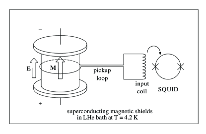
Figure 1: A schematic experimental setup for an EDM search.

Three solid state electron EDM experiments have been reported in literature. The first of these used a nickel-zinc ferrite, obtaining a limit of about $10^{-22}\mbox{ e$\cdot$cm}$ Vasilev and Kolycheva (1978). Another experiment, described in Ref. Heidenreich et al. (2005), obtained a limit that is lower by a factor of 40. This experiment employed a converse effect, in which a sample electric polarization appears when the sample is magnetized. The third experiment employs Gadolinium Gallium Garnet (GdGG), which has previously been identified as a promising paramagnetic system for this type of experiment Liu and Lamoreaux (2004). We have performed preliminary measurements, indicating that the anticipated sensitivity can be achieved, pending a $1/T$ behavior of the paramagnetic susceptibility to temperatures of order 10 mK. However, attaining an improved electron EDM limit requires that GdGG remains a simple paramagnetic system and that spin-glass or other effects do not enter down to temperatures of order 10 mK. Indeed, it is now known that such effects become very important near 0.2 K Schiffer et al. (1995), where the magnetic susceptibility reaches a peak value of $\chi=0.15$ (CGS units). This value is actually larger than the susceptibility given by the Curie-Weiss law, $\chi\propto(T-T_{c})^{-1}$, which describes the susceptibility of GdGG above 1 K, where $T_{c}\approx-2$ K for GdGG. We are continuing to investigate the ultimate sensitivity of a GdGG-based experiment, and the relaxation time of the spins remains to be determined. It is possible that this time will be long enough that extra noise due to spin fluctuations will be a limitation Budker et al. (2006), as we discuss below. In the meantime we have mounted a search for other materials whose properties make them attractive for conducting this type of an EDM experiment.

II The search for the best material

II.1 The magnetic susceptibility

For a solid state electron EDM experiment, materials with large magnetic susceptibility (or relative permeability) are desired. This is because, neglecting boundary effects (see Section III), the EDM-induced magnetization is given by

$$M=\chi kd_{e}E/\mu_{a},$$ (1)

where $\chi$ is the magnetic susceptibility, $k$ is the effective EDM enhancement factor in the material under study, $d_{e}$ is the electron EDM, $E$ is the applied electric field, and $\mu_{a}$ is the magnetic moment of the paramagnetic atoms or ions that carry the electron EDM ($\mu_{a}=8\mu_{B}$ for Gd⁺³, $\mu_{B}$ is the Bohr magneton). This assumes that all of the magnetization is due to the magnetic moments of the heavy atoms, that carry an EDM (a good approximation for all cases considered here). We see immediately that $\chi$ should be as large as possible. Note that the sample temperature does not explicitly enter into this formula.

Garnet ferrites with rare earth substitution can have large permeabilities at temperatures below 100 K. We have studied the complex permeability ($\mu=\mu^{\prime}-i\mu^{\prime\prime}$, $\mu=4\pi\chi$) of mixed Gadolinium-Yittrium iron garnets (GdYIG, chemical formula Gd_(3-x)Y_xFe₅O₁₂) down to 2 K Eckel et al. (2008). Our data show that for pure GdIG ceramic, $\mu^{\prime}=77$ at 4.2 K, and for mixed Gd_1.8Y_1.2Fe₅O₁₂ ceramic, $\mu^{\prime}=50$ at 4.2 K. The immediate conclusion is that at 4.2 K, in the absence of sample-shape effects, the EDM-induced magnetization in pure GdIG is enhanced by a factor of more than 300 compared to that in GdGG, which has $\chi=0.016$ at 4.2 K Schiffer et al. (1995). The present manuscript describes our study of the feasibility of an EDM experiment with GdIG.

II.2 The effective EDM enhancement factor and the internal electric field

The enhancement factor $k$ that appears in Eq. (1) determines the scale of the effective electric field acting on the Gd⁺³ ion EDM in GdIG. To calculate this, let us consider the energy shift $\delta$ resulting from a non-zero EDM of an ion in the lattice of an ionic solid. A naive estimate of this energy shift can be written down as follows:

$$\delta_{\text{naive}}\approx-d_{i}E_{\text{local}}\approx-\frac{\epsilon+2}{3}d_{i}E,$$ (2)

where $d_{i}$ is the Gd⁺³ ion EDM, $E_{\text{local}}$ is the local electric field at a Gd⁺³ ion site, $\epsilon$ is the dielectric constant of GdIG, and $E$ is the applied electric field. Here we used the Lorentz relation for the local field in a dielectric (in the approximation of a cubic crystal structure) Kittel (1996). The magnitude of $d_{i}$ induced by the electron EDM is calculated in Ref. Dzuba et al. (2002): $|d_{i}|\approx 2.2d_{e}$. With $\epsilon=15$, we get the naive estimate $\delta_{\text{naive}}\approx-13d_{e}E$.

A more rigorous calculation is presented in Refs. Mukhamedjanov et al. (2003); Dzuba et al. (2002); Kuenzi et al. (2002). The energy shift is expressed in terms of the displacement $x$ of the EDM-carrying ion with respect to its equilibrium position in the unit cell:

$$\delta\approx-0.1\frac{x}{a_{B}}\frac{d_{e}}{ea_{B}}\cdot 27.2\text{ eV},$$ (3)

where $a_{B}$ is the Bohr radius, $e$ is electron charge, and $27.2\text{ eV}$ is the atomic unit of energy. The Gd⁺³ ion displacement $x$ is related to the applied electric field through the dielectric constant: $x=(\epsilon_{ion}-1)E/12\pi en$, where $\epsilon_{ion}$ is the dielectric constant contribution due to ion displacement and $n\approx 10^{22}$ cm^-3 is the Gd density. We are assuming that the displacement of Fe ions is much smaller due to the stiffer Fe-O bond. The other contribution to the dielectric constant in GdIG is the “electronic polarizability” - the polarization of the individual ions in the electric field. We can estimate this contribution from the refractive index $n\approx 2.2$ of GdIG at optical frequencies, where the lattice polarizability does not contribute. Thus $\epsilon_{ion}\approx 15-2.2^{2}\approx 10$ is a reasonable estimate for the lattice polarizability. With this value, the EDM-induced energy shift in GdIG is:

$$\delta\approx-20d_{e}E.$$ (4)

Thus the effective enhancement factor is $k=20$. As pointed out in Ref. Dzuba et al. (2002), this is a conservative estimate, and the true result may be up to a factor of two larger. Note that the final value of $k$ is quite close to the naive estimate discussed above.

III The effect of the sample shape

Above we described two enhancement mechanisms for an EDM-induced signal in GdYIG ferrites: large magnetic permeability and local electric field enhancement by the crystal lattice. The combination of these makes this an attractive system for mounting an EDM search. It must be noted, however, that sample geometry-dependent demagnetizing fields eliminate part of the advantage of having a large-permeability material. It is well known, for example, that it is difficult to magnetize a thin disk of large-permeability magnetic material along its axis of symmetry (permanent magnets with such magnetization exist because their magnetization is saturated, i.e. their linear permeability is close to 1). This is explained by the Maxwell’s equation $\nabla\cdot\bm{B}=0$, combined with the relation $\bm{B}=\bm{H}+4\pi\bm{M}$ (CGS units). If a sample has some macroscopic magnetization $\bm{M}$, then on its surface $\nabla\cdot\bm{H}=-4\pi\nabla\cdot\bm{M}\neq 0$ gives rise to the “demagnetizing field” $\bm{H}$, which opposes the magnetization $\bm{M}$. The magnitude of this demagnetizing field depends on the sample geometry and permeability. For a high-permeability material the resultant magnetization can be much less than that in the case of no demagnetizing field, which happens for a long thin needle geometry, for example.

The demagnetizing field, and the sample magnetization, can be calculated exactly when the material is in the form of an ellipsoid Landau and Lifshitz (1980a), but not for a disk-shaped sample, which would be used an an EDM search (some approximate expressions for saturated hard ferromagnets are obtained in Refs. Joseph and Schlomann (1965); Joseph (1966); Arrott et al. (1979); Sato and Ishii (1989)). We used the finite-difference method to numerically solve Maxwell’s equations $\nabla\cdot\bm{B}=0$ and $\nabla\times\bm{H}=0$, with a cylindrical sample of radius $r$, thickness $h$, and permeability $\mu$. In such a geometry the magnetization is not uniform, but we can calculate the total magnetic flux $\Phi$ through a circular loop positioned on the surface of the cylinder halfway between its top and bottom. When $h\gg r$, there is no demagnetizing field, and $\Phi=4\pi M\pi r^{2}$, where $M$ is the EDM-induced magnetization given by Eq. (1). In general, however, we have to write

$$\Phi=g\cdot 4\pi M\pi r^{2},$$ (5)

where $g=g(h/r,\mu)$ is the flux suppression geometric factor that depends of the geometry and the permeability of the sample. The results of our numerical calculations, expressed as $g(h/r,\mu)$, are shown in Fig. 2.

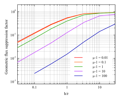
Figure 2: The magnetic flux suppression geometric factor for a permeable cylindrical sample.

There is clearly a significant suppression of the EDM-induced magnetic flux for a reasonable sample geometry ($h/r\simeq 1$) and for $\mu\simeq 50$. Certainly the suppression factor $g$ does not give the whole story, since there are several other geometry-dependent factors that enter into the final EDM sensitivity, such as the pickup loop area and inductance, as well as the electric field for a given experimentally achievable voltage applied to the sample. Further discussion of these factors can be found in Section V. It is also important to note that for $h/r\ll 1$, there is a significant suppression even for $\mu-1\ll 1$, as would be the case in a search for a nuclear Schiff moment, for example Bouchard et al. (2008). Therefore, in any magnetization-type EDM search, a thin disk-shaped sample would lead to a loss in sensitivity, instead samples with $h\simeq r$ must be used.

IV The magnetic noise measurements

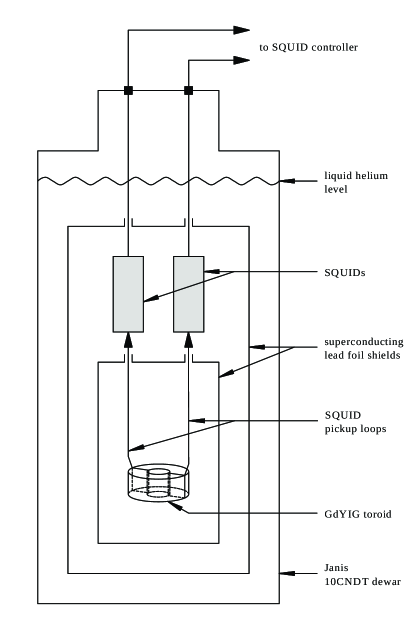
Figure 3: The experimental setup for magnetic noise measurements.

Even with a substantial signal suppression by the demagnetizing fields, it is possible, by carefully choosing the sample dimensions, to design an EDM search of formidable sensitivity. Before a full-scale experiment with Gd-containing ferrites is attempted, however, the intrinsic magnetic noise of the material must be measured. If this noise is greater than the magnetometer noise, the sensitivity of the EDM-induced magnetization measurement is reduced Budker et al. (2006).

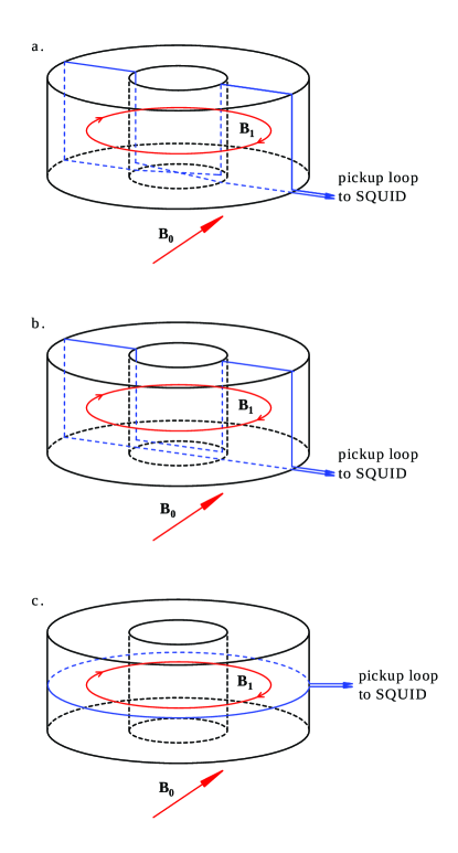
Figure 4: The three SQUID pickup loop geometries used for the magnetic noise measurements: a. pickup loop in the shape of figure-eight for external magnetic field rejection; b. U-shaped pickup loop for rejection of magnetic field lines internal to the toroid; c. pickup loop wound around the toroid perimeter to detect axial magnetic field. Magnetic field vectors are schematically shown in red. $B_{0}$ is the magnetic field outside the toroid. $B_{1}$ labels an azimuthal magnetic field line, looping around inside the toroid.

The setup used for the GdIG and GdYIG magnetic noise measurements is shown in Fig. 3. The sample is a sintered ceramic toroid with a square cross-section, outer diameter 3 cm, inner diameter 1 cm, and thickness 1 cm. Experiments were performed with ceramic samples of Gd₃Fe₅O₁₂, obtained from Pacific Ceramics Pac . The superconducting pickup loop was made from enamel-insulated niobium wire of thickness 0.003 in. It was connected to the input terminals of a Quantum Design DC thin-film SQUID sensor (model 50). The SQUIDs were connected to the control unit (model 5000) via 4-meter MicroPREAMP cables. The measurement bandwidth was limited to 1 kHz by an analog filter in the SQUID controller, to prevent aliasing. The intrinsic flux noise of the SQUID magnetometers in this frequency range was 2 $\mu\Phi_{0}$/$\sqrt{\rm Hz}$, which corresponds to magnetic field noise of several fT/$\sqrt{\rm Hz}$, the exact value depending on the area of each pickup loop. This noise level was always much less than the measured sample magnetization noise. The SQUID noise 1/f corner was around 0.1 Hz. The SQUIDs and the sample were mounted on G-10 holders, carefully fixed to minimize vibrations, and enclosed in superconducting shielding, made of 0.1-mm thick Pb foil, glued to the inner surfaces of two G-10 cylinders. The magnetic field shielding factor of our setup was greater than $10^{9}$. The entire setup was submerged in liquid helium inside a Janis model 10CNDT dewar. To dampen out vibrations, the dewar was mounted on rubber supports and placed on a 15” diameter support ring, comprising a partially inflated bicycle inner tube; however the residual vibrations of the SQUID pickup loops with the respect to the residual magnetic field gradients inside the superconducting magnetic shields were enough to cause the pronounced high-frequency (between 10 Hz and 1 kHz) peaks in the SQUID measurements shown in Fig. 5. Temperature was measured with a LakeShore model DT-670C-SD silicon diode temperature sensor, accurate to 0.1 K.

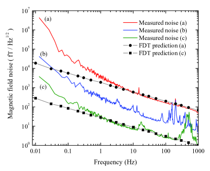
Figure 5: The results of the magnetic noise measurements. The curves are marked with the corresponding pickup loop geometry, shown in Fig. 4. Two noise expected from the fluctuation-dissipation theorem (FDT) for geometries (a) and (c) is also shown.

Magnetic noise measurements were done with several pickup-loop geometries to investigate the effect of the demagnetizing field on the noise. It is energetically favorable for the magnetic field lines to stay inside a high-permeability material, therefore most of the flux due to the magnetic noise in the material is confined inside the toroid, as indicated in Fig. 4. This flux can be detected by a SQUID pickup loop wound in the form of a figure-eight, i.e. in the gradiometer configuration (Fig. 4a). The spectrum of the measured magnetic field noise for this geometry is shown as the red curve marked (a) in Fig. 5. In this case, the magnetic field lines were closed inside the toroid, and, to a good approximation, there was no demagnetizing field (geometric factor $g=1$), therefore this was a measurement of the intrinsic magnetization noise of the ferrite sample.

To demonstrate that the observed magnetic field noise is due to the magnetization inside the material, rather than the magnetic field noise originating outside the sample, we performed noise measurements with a SQUID pickup loop wound in the U-shaped form, i.e. in the magnetometer configuration perpendicular to the plane of the toroid (Fig. 4b). The spectrum of the measured magnetic field noise for this geometry is shown as the green curve marked (b) in Fig. 5. In this case, the flux due to the magnetic field lines that were closed inside the toroid was not coupled to the SQUID, and only the magnetic field that entered or exited the toroid was detected.

Finally, to simulate the geometry of an EDM experiment as closely as possible, we measured the magnetic field noise that couples to the SQUID with the pickup loop wound around the perimeter of the sample, as shown in Fig. 4c. In this case, the magnetic flux noise was given by the GdIG magnetization noise, reduced by the appropriate geometric factor that takes into account the demagnetizing field, as in Eq. (5). The results are shown as the blue curve marked (c) in Fig. 5. The pronounced peaks in all three of the noise data sets are caused by vibrations, as discussed above.

Let us proceed to the analysis and discussion of these magnetic noise data. The magnetization noise in a material with a known complex permeability $\mu=\mu^{\prime}-i\mu^{\prime\prime}$ can be calculated using the fluctuation-dissipation theorem (FDT) Landau and Lifshitz (1980b):

$$(M^{2})_{\omega}=\frac{1}{2\pi V}\frac{k_{B}T}{\omega}\mu^{\prime\prime}(\omega),$$ (6)

where $(M^{2})_{\omega}$ is the power spectral density of the magnetization noise at frequency $\omega$, $V$ is the sample volume, $k_{B}$ is Boltzmann’s constant, and $T$ is temperature. Complex permeability has been measured in GdIG and mixed GdYIG ceramics in a range of temperatures (2 K to 295 K) and frequencies (100 Hz to 200 MHz) Eckel et al. (2008). In order to compare our noise measurements with the FDT, we measured the complex permeability of GdIG at 4.2 K in the frequency range of 0.01 Hz to 1 kHz. This was done by winding two 23-turn excitation coils in series, one around the GdIG toroid, and one around a toroid of the same dimensions, but made of G-10. Each of the toroids was connected to a SQUID via a one-turn pickup loop. The GdIG complex permeability was extracted from the relative amplitude and phase shift of the SQUID signals, as a sinusoidal current with frequency ranging between 0.01 Hz and 1 kHz was applied to the excitation coil. The resulting values of $\mu^{\prime\prime}$ were used in Eq. (6) to generate the magnetic field noise expected from the FDT. This is shown by circles in Fig. 5, in the case of no demagnetizing fields (geometric factor $g=1$), which is a good approximating for geometry (a).

For frequencies greater than approximately 5 Hz, there is very good agreement with the magnetic field noise measured with the SQUID for this geometry. We interpret this as a verification of the validity of the FDT for our system in this frequency range. For lower frequencies, however, the FDT seems to systematically underestimate the magnetic field noise, by as much as two orders of magnitude. We speculate that the excess magnetic field noise is due to very slowly-relaxing degrees of freedom, which come to thermal equilibrium on the time scales much longer than the duration of our experimental run (a few hours) Crisanti and Ritort (2003). For such degrees of freedom, the effective noise temperature that should be used in Eq. (6) is much greater than 4.2 K, thus they contribute greater noise.

In Section III we discussed how the sample shape affects the EDM signal, presumably the magnetization noise is also reduced by the same demagnetizing fields. This is confirmed by the measurements of the noise with the SQUID pickup loop around the sample perimeter (Fig 4c). Indeed, if the FDT prediction (6) is multiplied by the geometric factor appropriate for the sample dimensions ($h/r=0.67$ resulting in $g=0.017$), the result is the expected magnetic noise in the geometry of Fig 4c. This is shown by the squares in Fig 5, and once again, the agreement with the SQUID measurements is remarkable above frequencies on the order of a few Hz. We can therefore conclude that we predict the magnetic field noise in any geometry by taking into account the geometric factor, as described in Section III.

V The projected sensitivity of an experiment with GdIG

Having measured the magnetization noise in GdIG, we can estimate the statistical sensitivity of an EDM experiment with a GdIG sample. Combining Eqs. (1) and (5), we obtain the EDM-induced magnetic flux through a pickup loop around a cylindrical sample:

$$\Phi_{\text{EDM}}=g\pi r^{2}\cdot 4\pi\chi\frac{kd_{e}E}{8\mu_{B}},$$ (7)

where all the symbols have been defined previously. The statistical sensitivity is limited by the material magnetization noise, given by Eq. (6), the resulting magnetic flux noise through the pickup loop is given by:

$$\Phi_{\text{noise}}=g\pi r^{2}\cdot 4\pi\sqrt{\frac{1}{4\pi^{3}r^{2}h}\frac{k_{B}T\mu^{\prime\prime}}{f}},$$ (8)

where $f=\omega/2\pi$ is the electric field reversal frequency. We can now express the statistical sensitivity in terms of experimental parameters:

$$\delta d_{e}=\frac{4\mu_{B}}{\pi\chi kV_{0}}\sqrt{\frac{h}{\pi r^{2}}\frac{k_{B}T\mu^{\prime\prime}}{f}},$$ (9)

where we introduced the amplitude $V_{0}$ of the voltage applied to the electrodes. Interestingly, the geometric factor $g$ does not enter this sensitivity estimate, this is because it appears in both the EDM-induced flux and the noise-induced flux. If the magnetization noise had turned out to be lower than the intrinsic noise of the SQUID, the geometric factor would have entered into the sensitivity estimate (so would the SQUID sensitivity and the number of turns of the SQUID pickup loop, see Appendix A). Equation (9) assumes a disc-shaped geometry, but the sample dimensions have not been specified. It is clear that the best sample is a thin disc of large radius: decreasing the thickness $h$ increases the applied electric field for a given voltage $V_{0}$, and increasing the radius $r$ increases the sample volume, which decreases the magnetization noise, according to Eq. (6). It is also clearly advantageous to reverse the electric field as fast as possible, however displacement currents limit the maximum realistic reversal frequency to 10 Hz (see below for more detailed discussion of systematics). For a quantitative estimate of the EDM sensitivity we take the following experimental parameters: $V_{0}=10$ kV, $h=0.1$ cm, $r=3$ cm, $f=10$ Hz, resulting in $\delta d_{e}\simeq 4\times 10^{-24}\mbox{ e$\cdot$cm}/\mbox{$\sqrt{\rm Hz}$}$. After 10 days of integration, a statistical sensitivity at the level of

$$\delta d_{e}\simeq 3\times 10^{-27}\mbox{ e$\cdot$cm}$$ (10)

can be achieved.

A number of systematic concerns for a solid state sample-based EDM search have been outlined in Ref. Lamoreaux (2002). With a ferromagnetic system, magnetic hysteresis is also crucially important. The main concern is electric field-correlated sample magnetization caused by the magnetic fields generated by displacement currents. It should be noted that these magnetic fields tend to be perpendicular to the EDM-induced magnetization, but some degree of misalignment is inevitable. The current associated with applying 10 kV to a 300 pF sample at 10 Hz reversal frequency is about 30 $\mu$A, which gives rise to magnetic field of order $H_{d}\simeq 2\times 10^{-6}$ A/cm. The resulting remanent magnetization $M_{d}$, present after the current is brought back down to zero, can be calculated from the parameters of the Raleigh hysteresis loops measured for GdIG in Ref. Eckel et al. (2008). Taking a reduction of a factor of 10 due to perpendicularity, the resulting magnetization along the electric field is $M_{d}^{||}\simeq 10^{-12}$ emu/cm³. According to Eq. (5), the induced magnetic flux is suppressed by the geometric factor, which, for a disc of $h=0.1$ cm and $r=3$ cm, is approximately $10^{-3}$. The resulting systematic is at the level of statistical sensitivity given in Eq. (10).

Another possible systematic is the so-called magneto-electric effect Landau and Lifshitz (1980a). The applied electric field induces a strain in the sample (electrostriction), which then induces a magnetization correlated with the electric field, provided the sample already possesses some non-zero magnetization (inverse magnetostriction). This effect is described by the term $\gamma E^{2}H^{2}$ (we omit the tensor indices) in the electromagnetic free energy, which is allowed by both the parity and the time-reversal symmetries. This has been observed in YIG O’Dell (1967) and GdIG Mercier (1974). The “magneto-electric susceptibility” $\beta_{M}$ is defined in the following manner: $M=\beta_{m}(H_{0})E^{2}$, where $H_{0}$ is the external magnetic field, $E$ is the applied electric field, and $M$ is the resulting magnetization. For GdIG single crystals in the low-field limit ($H_{0}<30$ Oe), the magneto-electric susceptibility was measured to be: $\beta_{m}(H_{0})\simeq 10^{-8}\cdot H_{0}(\text{Oe})$ emu/cm³, where $H_{0}$ is expressed in Oestreds Mercier (1974). For a poly-crystalline sample, this should be reduced by a factor of 3 (the average over crystallite orientations). With the electric field of 100 kV/cm, and assuming 1% reversal accuracy, the external magnetic field $H_{0}$ has to be kept below $3\times 10^{-7}$ Oe in order to control this systematic at the level of statistical sensitivity. This appears feasible with a combination of Metglas magnetic shielding and superconducting lead shields.

Finally, we point out that, if a gradiometer setup is used with a large-permeability sample, the gradiometer tuning has to be adjusted, see Appendix B for analysis.

VI Conclusion and outlook

We have performed a detailed feasibility study for an electron electric dipole moment search with a solid ceramic sample of Gadolinium iron garnet. This material is attractive because it is an excellent insulator, and it maintains a high magnetic permeability down to liquid helium temperatures, $\mu=77$ at 4.2 K, which enhances the EDM-induced magnetization and allows the design of an experiment based on SQUID-magnetometer detection and superconducting magnetic shielding. In addition, the electric field acting on the electron EDM is amplified by the crystalline lattice polarizability, resulting in an effective EDM enhancement factor of 20. When calculating the EDM-induced magnetic flux, one must take into account the demagnetizing field, which suppresses it by a factor that depends on the sample geometry and permeability. The dominant sensitivity limitation in the proposed experiment, however, is the intrinsic magnetization noise of the Gadolinium iron garnet samples at 4.2 K. We measured this noise and verified that our data are consistent with the fluctuation-dissipation theorem in the 5 Hz to 1 kHz frequency range. At lower frequencies the noise seems to be dominated by magnetic degrees of freedom that are out of equilibrium with the liquid helium heat bath. We also verified the expected scaling of the noise-induced magnetic flux with the sample geometry. We estimate the statistical sensitivity of an EDM search based on a solid GdIG sample to be $3\times 10^{-27}\mbox{ e$\cdot$cm}$ after 10 days of averaging. This is slightly above the present experimental limit, but such a measurement would still be highly valuable, given the completely different methods and systematics involved. We also estimate the most likely systematics: the magnetic hysteresis and the magneto-electric effect. Our analysis shows that it should be possible to control these at the level of statistical sensitivity.

It seems feasible that the magnetic noise can be reduced by diluting the GdIG powder with a non-magnetic mixer (such as teflon) prior to pressing the ceramic samples, Another possibility is substituting some of the Fe ions in the lattice with paramagnetic ions, such as Ga, making mixed Gd₃Fe_(5-x)Ga_xO₁₂ ceramics. This will probably reduce the magnetic susceptibility as well as the magnetization noise, but, by carefully choosing the sample dimensions, this loss can be compensated by an improved geometric factor. Yittrium-substituted Gadolinium garnets with chemical formula Gd_3-xY_xFe₅O₁₂ have been studied in Ref. Eckel et al. (2008), and the measured complex permeability at 4.2 K leads to a poorer EDM sensitivity estimate for such ceramics. We have, in addition, identified an extremely promising material where the sensitivity gain is provided by the crystal lattice, rather than by the large magnetic permeability Mukhamedjanov and Sushkov (2005). This material is gadolinium molybdate (chemical formula Gd₂(MoO₄)₃), which is a ferroelectric-ferroelastic with Curie temperature of 160^∘C and spontaneous polarization of 0.25 $\mu$C/cm². Preliminary estimates and measurements indicate that a two-order of magnitude improvement over the present limit is possible with this material. We are currently pursuing further studies of Gd₂(MoO₄)₃, as well as other magnetic ferroelectrics.

VII Acknowledgements

The authors acknowledge useful discussions with Woo-Joong Kim, David DeMille, Jack Harris, Oleg Sushkov, Dima Budker, Michel Devoret, and Larry Hunter.

Appendix A The multi-turn SQUID pickup loop

If the sample magnetization noise happens to be below the SQUID noise, the EDM sensitivity is limited by the SQUID noise. To achieve the best coupling of the sample flux to the SQUID, a multi-turn pickup loop may be used. This appendix shows that having a several-turn pickup loop may be advantageous, and suggests how the number of turns may be optimized.

Let us denote by $N$ the number of turns of the SQUID superconducting pickup loop around the sample, $A$ is the area of the sample. The circuit is schematically shown in Fig. 1. Suppose the magnetic field through the pickup loop varies sinusoidally as a function of time, with frequency $\omega$: $B=B_{0}e^{-i\omega t}$. The electromotive force around the circuit is then given by Faraday’s law: ${\mathcal{E}}=i\omega NAB_{0}e^{-i\omega t}=i\omega N\Phi$, where we define the magnetic flux $\Phi=BA$. The current in the circuit is given by $I={\mathcal{E}}/(Z_{\text{in}}+Z_{p})$, where the impedances of the SQUID input coil and the pickup loop are in the denominator. Expressing these inductive impedances as $Z=i\omega L$ results in $I=N\Phi/(L_{\text{in}}+L_{p}^{(N)})$, where $L_{\text{in}}\approx 1.5$ $\mu$H is the input coil self-inductance and $L_{p}^{(N)}$ is the self-inductance of the N-turn pickup loop. The flux that is coupled to the SQUID is given by $\Phi_{\text{SQ}}=M_{\text{in}}I$, where $M_{\text{in}}\approx 10$ nH is the SQUID-input coil mutual inductance. Thus we finally have:

$$\Phi_{\text{SQ}}=\frac{NM_{\text{in}}}{L_{\text{in}}+L_{p}^{(N)}}\Phi.$$ (11)

Having a several-turn pickup loop improves the flux coupling to the SQUID, but only until the pickup coil inductance reaches $L_{p}^{(N)}\approx L_{\text{in}}$. If the number of turns is increased further, so that $L_{p}^{(N)}\gg L_{\text{in}}$, the coupling deteriorates, since $L_{p}^{(N)}$ scales as $N^{2}$. The optimal number of turns can be calculated from Eq. (11), given the dimensions of the sample and the superconducting wire, and using an expression for the inductance of a multi-turn coil Terman (1943).

Appendix B Detuning of the Gradiometer Condition due to Sample Permeability

Previous work Liu and Lamoreaux (2004) employed two superconducting pickup loops around the sample, operated in a concentric loop planar gradiometer configuration, to reduce magnetic field noise. Unfortunately, the permeability of the sample alters the pickup loop inductances, and spoils the gradiometer tuning, and reduces the experiment sensitivity slightly because the loop inductance is increased. In the case of a single loop or radius $a$ around an infinitely long cylinder of permeability $\mu$ and radius $b$, the increase in inductance is Smythe (1950)

$$\delta L=2\mu_{0}a^{2}\int_{0}^{\infty}\Phi(k)[K_{1}(ka)]^{2}dk$$ (12)

where $\mu_{0}$ is the permeability of free space, $K_{1}(ka)$ is the first order modified Bessel function, and

$$\Phi(k)={(\mu-1)kbI_{0}(kb)I_{1}(kb)\over(\mu-1)kbK_{0}(kb)I_{1}(kb)+1}\approx{I_{0}(kb)\over K_{0}(kb)}$$ (13)

where $I_{0}$ and $K_{0}$ are the zero-order modified Bessel functions, and the approximation holds when $\mu>>1$. We use SI units in this Appendix. The effect of finite length is small, provided that length $\ell\geq 2b$, which is the case for the experiment. In the case $a=b$ for a loop directly on a cylinder, $\delta L\approx 6\mu_{0}a\approx 0.1\ \mu$H, for $a=1.2$ cm, a 20% effect. When $a=\sqrt{2}b$, $\delta L=0.02\ \mu$H, a much smaller effect. The loss in sensitivity is around 10%, leaving the principal problem due to this effect as the detuning of the gradiometer condition, which is temperature dependent, and of order 10%. Usually, gradiometers are fabricated to provide 1% common mode rejection. Thus, we see a substantial limitation to the degree of common mode rejection possible when there is a permeable sample in the central loop. In principle, the loop areas could be adjusted to cancel gradients at a particular temperature, but introduces difficulties if temperature variation is employed to test for systematic effects.

References

- Balazs et al. (2005) C. Balazs, M. Carena, A. Menon, D. E. Morrissey, and C. E. M. Wagner, Physical Review D (Particles and Fields) 71, 075002 (2005).
- Regan et al. (2002) B. C. Regan, E. D. Commins, C. J. Schmidt, and D. DeMille, Physical Review Letters 88, 071805 (2002).
- Hudson et al. (2002) J. J. Hudson, B. E. Sauer, M. R. Tarbutt, and E. A. Hinds, Physical Review Letters 89, 023003 (2002).
- Kawall et al. (2004) D. Kawall, F. Bay, S. Bickman, Y. Jiang, and D. DeMille, Physical Review Letters 92, 133007 (2004).
- Kawall et al. (2005) D. Kawall, Y. V. Gurevich, C. Cheung, S. Bickman, Y. Jiang, and D. DeMille, Physical Review A 72, 064501 (2005).
- Stutz and Cornell (2004) R. P. Stutz and E. A. Cornell, Bull. Am. Phys. Soc. 89, 76 (2004).
- Weiss et al. (2003) D. S. Weiss, F. Fang, and J. Chen, Bull. Am. Phys. Soc. APR03, J1.008 (2003).
- Ledbetter et al. (2005) M. P. Ledbetter, I. M. Savukov, and M. V. Romalis, Physical Review Letters 94, 060801 (2005).
- Bouchard et al. (2008) L. S. Bouchard, A. O. Sushkov, D. Budker, J. J. Ford, and A. S. Lipton, Physical Review A 77, 022102 (2008).
- Shapiro (1968) F. L. Shapiro, Soviet physics, Uspekhi 11, 345 (1968).
- Lamoreaux (2002) S. K. Lamoreaux, Physical Review A 66, 022109 (2002).
- Vasilev and Kolycheva (1978) B. V. Vasilev and E. V. Kolycheva, Soviet Physics - JETP 47, 243 (1978).
- Heidenreich et al. (2005) B. J. Heidenreich, O. T. Elliott, N. D. Charney, K. A. Virgien, A. W. Bridges, M. A. McKeon, S. K. Peck, J. D. Krause, J. E. Gordon, L. R. Hunter, et al., Physical Review Letters 95, 253004 (2005).
- Liu and Lamoreaux (2004) C.-Y. Liu and S. K. Lamoreaux, Modern Physics Letters A 19, 1235 (2004).
- Schiffer et al. (1995) P. Schiffer, A. P. Ramirez, D. A. Huse, P. L. Gammel, U. Yaron, D. J. Bishop, and A. J. Valentino, Physical Review Letters 74, 2379 (1995).
- Budker et al. (2006) D. Budker, S. K. Lamoreaux, A. O. Sushkov, and O. P. Sushkov, Physical Review A 73, 022107 (2006).
- Eckel et al. (2008) S. Eckel, A. O. Sushkov, and S. K. Lamoreaux, arXiv:0810.2770v1.
- Kittel (1996) C. Kittel, Introduction to Solid State Physics (Wiley & Sons, Neew York, 1996), 7th ed.
- Dzuba et al. (2002) V. A. Dzuba, O. P. Sushkov, W. R. Johnson, and U. I. Safronova, Physical Review A 66, 032105 (2002).
- Mukhamedjanov et al. (2003) T. N. Mukhamedjanov, V. A. Dzuba, and O. P. Sushkov, Physical Review A 68, 042103 (2003).
- Kuenzi et al. (2002) S. A. Kuenzi, O. P. Sushkov, V. A. Dzuba, and J. M. Cadogan, Physical Review A 66, 032111 (2002).
- Landau and Lifshitz (1980a) L. D. Landau and E. M. Lifshitz, Electrodynamics of continuous media (Butterworths-Heinemann, London, 1980a), 3rd ed.
- Joseph and Schlomann (1965) R. I. Joseph and E. Schlomann, Journal of Applied Physics 36, 1579 (1965).
- Joseph (1966) R. I. Joseph, Journal of Applied Physics 37, 4639 (1966).
- Arrott et al. (1979) A. Arrott, B. Heinrich, and A. Aharoni, Magnetics, IEEE Transactions on 15, 1228 (1979).
- Sato and Ishii (1989) M. Sato and Y. Ishii, Journal of Applied Physics 66, 983 (1989).
- (27) Web address: http://pceramics.com/.
- Landau and Lifshitz (1980b) L. D. Landau and E. M. Lifshitz, Statistical physics, pt. 1 (Butterworths-Heinemann, London, 1980b), 3rd ed.
- Crisanti and Ritort (2003) A. Crisanti and F. Ritort, Journal of Physics A: Mathematical and General 36, R181 (2003).
- O’Dell (1967) T. H. O’Dell, Philosophical Magazine 16, 487 (1967).
- Mercier (1974) M. Mercier, International Journal of Magnetism 6, 77 (1974).
- Mukhamedjanov and Sushkov (2005) T. N. Mukhamedjanov and O. P. Sushkov, Physical Review A 72, 034501 (2005).
- Terman (1943) F. E. Terman, Radio Engineers’ Handbook (MvGraw-Hill, New York and London, 1943).
- Smythe (1950) W. R. Smythe, Static and Dynamic Electricity (McGraw-Hill, New York, 1950), chap. 8, prob. 15.