Explicit combinatorial interpretation
of Kerov character polynomials
as numbers of permutation factorizations

Abstract.

We find an explicit combinatorial interpretation of the coefficients of Kerov character polynomials which express the value of normalized irreducible characters of the symmetric groups $\mathfrak{S}(n)$ in terms of free cumulants $R_{2},R_{3},\dots$ of the corresponding Young diagram. Our interpretation is based on counting certain factorizations of a given permutation.

1. Introduction

1.1. Generalized Young diagrams

We are interested in the asymptotics of irreducible representations of the symmetric groups $\mathfrak{S}(n)$ for $n\to\infty$ in the scaling of balanced Young diagrams which means that we consider a sequence $(\lambda^{(n)})$ of Young diagrams with a property that $\lambda^{(n)}$ has $n$ boxes and $O(\sqrt{n})$ rows and columns. This scaling makes the graphical representations of Young diagrams particularly useful; in this article we will use two conventions for drawing Young diagrams: the French (presented on Figure 1) and the Russian one (presented on Figure 2). Notice that the graphs in the Russian convention are created from the graphs in the French convention by rotating counterclockwise by $\frac{\pi}{4}$ and by scaling by a factor $\sqrt{2}$.

Any Young diagram drawn in the French convention can be identified with its graph which is equal to the set $\{(x,y):0\leq x,0\leq y\leq f(x)\}$ for a suitably chosen function $f:\mathbb{R}_{+}\rightarrow\mathbb{R}_{+}$, where $\mathbb{R}_{+}=[0,\infty)$. It is therefore natural to define the set of generalized Young diagrams $\mathbb{Y}$ (in the French convention) as the set of bounded, non-increasing functions $f:\mathbb{R}_{+}\rightarrow\mathbb{R}_{+}$ with a compact support; in this way any Young diagram can be regarded as a generalized Young diagram.

Figure 1. Young diagram $(4,3,1)$ drawn in the French convention

We can identify a Young diagram drawn in the Russian convention with its profile, see Figure 2. It is therefore natural to define the set of generalized Young diagrams $\mathbb{Y}$ (in the Russian convention) as the set of functions $f:\mathbb{R}\rightarrow\mathbb{R}_{+}$ which fulfill the following two conditions:

• $f$ is a Lipschitz function with constant $1$, i.e. $|f(x)-f(y)|\leq|x-y|$,

• $f(x)=|x|$ if $|x|$ is large enough.

Figure 2. Young diagram $(4,3,1)$ drawn in the Russian convention. The profile of the diagram has been drawn in the solid line.

At the first sight it might seem that we have defined the set $\mathbb{Y}$ of generalized Young diagrams in two different ways, but we prefer to think that these two definitions are just two conventions (French and Russian) for drawing the same object. This will not lead to confusions since it will be always clear from the context which of the two conventions is being used.

The setup of generalized Young diagrams makes it possible to speak about dilations of Young diagrams. In the geometric language of French and Russian conventions such dilations simply correspond to dilations of the graph. Formally speaking, if $f\in\mathbb{Y}$ is a generalized Young diagram (no matter in which convention) and $s>0$ is a real number we define the dilated diagram $sf\in\mathbb{Y}$ by the formula

$$(sf)(x)=sf\left(\frac{x}{s}\right).$$

This notion of dilation is very useful in the study of balanced Young diagrams because if $(\lambda^{(n)})_{n}$ is a sequence of balanced Young diagrams we may for example ask questions about the limit of the sequence $\frac{1}{\sqrt{n}}\lambda^{(n)}$ [LS77, VK77].

1.2. Normalized characters

Any permutation $\pi\in\mathfrak{S}(k)$ can be also regarded as an element of $\mathfrak{S}(n)$ if $k\leq n$ (we just declare that $\pi\in\mathfrak{S}(n)$ has additional $n-k$ fixpoints). For any $\pi\in\mathfrak{S}(k)$ and an irreducible representation $\rho^{\lambda}$ of the symmetric group $\mathfrak{S}(n)$ corresponding to the Young diagram $\lambda$ we define the normalized character

$$\Sigma^{\lambda}_{\pi}=\begin{cases}\underbrace{n(n-1)\cdots(n-k+1)}_{k\text{ factors}}\frac{\operatorname{Tr}\rho^{\lambda}(\pi)}{\text{dimension of $\rho^{\lambda}$}}&\text{if }k\leq n,\\ 0&\text{otherwise.}\end{cases}$$

One of the reasons why such normalized characters are so useful in the asymptotic representation theory is that, as we shall see in Section 4, one can extend the definition of $\Sigma^{\lambda}_{\pi}$ to the case when $\lambda\in\mathbb{Y}$ is a generalized Young diagram; furthermore computing their values will turn out to be easy.

Particularly interesting are the values of characters on cycles, therefore we will use the notation

$$\Sigma^{\lambda}_{k}=\Sigma^{\lambda}_{(1,2,\dots,k)},$$

where we treat the cycle $(1,2,\dots,k)$ as an element of $\mathfrak{S}(k)$ for any integer $k\geq 1$.

1.3. Free cumulants

Let $\lambda$ be a (generalized) Young diagram. We define its free cumulants $R_{2}^{\lambda},R_{3}^{\lambda},\dots$ by the formula

(1) $$R_{k}^{\lambda}=\lim_{s\to\infty}\frac{1}{s^{k}}\Sigma^{s\lambda}_{k-1},$$

in other words each free cumulant is asymptotically the dominant term of the character on a cycle of appropriate length in the limit when the Young diagram tends to infinity.

From the above definition it is clear that free cumulants should be interesting for investigations of the asymptotics of characters of symmetric groups, but it is not obvious why the limit should exist and if there is some direct way of calculating it. In Sections 2 and 3 we will review some more conventional definitions of free cumulants and some more direct ways of calculating them.

One of the reasons why free cumulants are so useful in the asymptotic representation theory is that they are homogeneous with respect to dilations of the Young diagrams, namely

$$R^{s\lambda}_{k}=s^{k}R^{\lambda}_{k};$$

in other words the degree of the free cumulant $R_{k}$ is equal to $k$. This property is an immediate consequence of (1) but it also follows from more conservative definitions of free cumulants.

In fact, the notion of free cumulants origins from the work of Voiculescu [Voi86] where they appeared as coefficients of an $R$-series which turned out to be useful in description of free convolution in the context of free probability theory [VDN92]. The name of free cumulants was coined by Speicher [Spe98] who found their combinatorial interpretation and their relations with the lattice of non-crossing partitions [Spe93]. Since free probability theory is closely related to the random matrix theory [Voi91] free cumulants quickly became an important tool not only within the framework of free probability but in the random matrix theory as well.

1.4. Kerov character polynomials

The following surprising fact is fundamental for this article: it turns out that free cumulants can be used not only to provide asymptotic approximations for the characters of symmetric groups, but also for exact formulas. Kerov during a talk in Institut Henri Poincaré in January 2000 [Ker00] announced the following result (the first published proof was given by Biane [Bia03]): for each permutation $\pi$ there exists a universal polynomial $K_{\pi}$ with integer coefficients, called Kerov character polynomial, with a property that

(2) $$\Sigma^{\lambda}_{\pi}=K_{\pi}(R_{2}^{\lambda},R_{3}^{\lambda},\dots)$$

holds true for any (generalized) Young diagram $\lambda$. We say that Kerov polynomial is universal because it does not depend on the choice of $\lambda$. In order to keep the notation simple we make the dependence of the characters and of the free cumulants on $\lambda$ implicit and we write

$$\Sigma_{\pi}=K_{\pi}(R_{2},R_{3},\dots).$$

As usual, we are mostly concerned with the values of the characters on the cycles, therefore we introduce special notation for such Kerov polynomials

$$\Sigma_{k}=K_{k}(R_{2},R_{3},\dots).$$

Kerov also found the leading term of the Kerov polynomial:

(3) $$\Sigma_{k}=R_{k+1}+(\text{terms of degree at most $k-1$})$$

which has (1) as an immediate consequence.

The first few Kerov polynomials $K_{k}$ are as follows [Bia01]:

$$\Sigma_{1} =R_{2},$$

$$\Sigma_{2} =R_{3},$$

$$\Sigma_{3} =R_{4}+R_{2},$$

$$\Sigma_{4} =R_{5}+5R_{3},$$

$$\Sigma_{5} =R_{6}+15R_{4}+5R_{2}^{2}+8R_{2},$$

$$\Sigma_{6} =R_{7}+35R_{5}+35R_{3}R_{2}+84R_{3}.$$

Based on such numerical evidence Kerov formulated during his talk [Ker00] the following conjecture.

Conjecture 1.1 (Kerov).

The coefficients of Kerov character polynomials $K_{k}$ ($k\geq 1$) are non-negative integers.

Biane [Bia03] stated a very interesting conjecture that the underlying reason for positivity of the coefficients of Kerov polynomials is that they are equal to cardinalities of some combinatorial objects. Biane provided also some heuristics what these combinatorial objects could be (we postpone the details until Section 1.11.1).

Since then a number of partial answers were found. Śniady [Śni06a] found explicitly the next term (with degree $k-1$) in the expansion (3) (the form of this next term was conjectured by Biane [Bia03]). Goulden and Rattan [GR07] found an explicit but complicated formula for the coefficients of Kerov polynomials. These results, however, did not shed too much light into possible combinatorial interpretations of Kerov character polynomials.

Some light on the possible combinatorial interpretation of Kerov polynomials was shed by the following result proved by Biane in the aforementioned paper [Bia03] and Stanley [Sta02].

Theorem 1.2 (Linear terms of Kerov polynomials).

For all integers $l\geq 2$ and $k\geq 1$ the coefficient of $R_{l}$ in the Kerov polynomial $K_{k}$ is equal to the number of pairs $(\sigma_{1},\sigma_{2})$ of permutations $\sigma_{1},\sigma_{2}\in\mathfrak{S}(k)$ such that $\sigma_{1}\circ\sigma_{2}=(1,2,\dots,k)$ and such that $\sigma_{2}$ consists of one cycle and $\sigma_{1}$ consists of $l-1$ cycles.

For a permutation $\pi$ we denote by $C(\pi)$ the set of cycles of $\pi$. Féray [Fér09] extended the above result to the quadratic terms of Kerov polynomials.

Theorem 1.3 (Quadratic terms of Kerov polynomials).

For all integers $l_{1},l_{2}\geq 2$ and $k\geq 1$ the coefficient of $R_{l_{1}}R_{l_{2}}$ in the Kerov polynomial $K_{k}$ is equal to the number of triples $(\sigma_{1},\sigma_{2},q)$ with the following properties:

• $\sigma_{1},\sigma_{2}$ is a factorization of the cycle; in other words $\sigma_{1},\sigma_{2}\in\mathfrak{S}(k)$ are such that $\sigma_{1}\circ\sigma_{2}=(1,2,\dots,k)$;

• $\sigma_{2}$ consists of two cycles and $\sigma_{1}$ consists of $l_{1}+l_{2}-2$ cycles;

• $q:C(\sigma_{2})\rightarrow\{l_{1},l_{2}\}$ is a surjective map on the two cycles of $\sigma_{2}$;

• for each cycle $c\in C(\sigma_{2})$ there are at least $q(c)$ cycles of $\sigma_{1}$ which intersect nontrivially $c$.

In fact, Féray [Fér09] managed also to prove positivity of the coefficients of Kerov character polynomials by finding some combinatorial objects with appropriate cardinality, but his proof was so complicated that the resulting combinatorial objects were hardly explicit in more complex cases. We compare this work with our new result in Section 8

1.5. The main result: explicit combinatorial interpretation of the coefficients of Kerov polynomials

The following theorem is the main result of the paper: it gives a satisfactory answer for the Kerov conjecture by providing an explicit combinatorial interpretation of the coefficients of the Kerov polynomials. It was formulated for the first time as a conjecture in June 2008 by Valentin Féray and Piotr Śniady after some computer experiments concerning the coefficient of $R_{2}^{3}$ in Kerov polynomials $K_{7}$ and $K_{9}$. The original formulation of the conjecture was Theorem 7.1; the form below was pointed out by Philippe Biane in a private communication.

Theorem 1.4 (The main result).

Let $k\geq 1$ and let $s_{2},s_{3},\dots$ be a sequence of non-negative integers with only finitely many non-zero elements. The coefficient of $R_{2}^{s_{2}}R_{3}^{s_{3}}\cdots$ in the Kerov polynomial $K_{k}$ is equal to the number of triples $(\sigma_{1},\sigma_{2},q)$ with the following properties:

1. $\sigma_{1},\sigma_{2}$ is a factorization of the cycle; in other words $\sigma_{1},\sigma_{2}\in\mathfrak{S}(k)$ are such that $\sigma_{1}\circ\sigma_{2}=(1,2,\dots,k)$;

2. the number of cycles of $\sigma_{2}$ is equal to the number of factors in the product $R_{2}^{s_{2}}R_{3}^{s_{3}}\cdots$; in other words $|C(\sigma_{2})|=s_{2}+s_{3}+\cdots$;

3. the total number of cycles of $\sigma_{1}$ and $\sigma_{2}$ is equal to the degree of the product $R_{2}^{s_{2}}R_{3}^{s_{3}}\cdots$; in other words $|C(\sigma_{1})|+|C(\sigma_{2})|=2s_{2}+3s_{3}+4s_{4}+\cdots$;

4. $q:C(\sigma_{2})\rightarrow\{2,3,\dots\}$ is a coloring of the cycles of $\sigma_{2}$ with a property that each color $i\in\{2,3,\dots\}$ is used exactly $s_{i}$ times (informally, we can think that $q$ is a map which to cycles of $C(\sigma_{2})$ associates the factors in the product $R_{2}^{s_{2}}R_{3}^{s_{3}}\cdots$);

5. for every set $A\subset C(\sigma_{2})$ which is nontrivial (i.e., $A\neq\emptyset$ and $A\neq C(\sigma_{2})$) there are more than $\sum_{i\in A}\big{(}q(i)-1\big{)}$ cycles of $\sigma_{1}$ which intersect $\bigcup A$.

A careful reader may notice that condition (b) in the above theorem is redundant since it is implied by condition (d); we decided to keep it for the sake of clarity. We postpone presenting interpretations of condition (e) until Section 1.8 and Section 1.9.

One can easily see that Theorem 1.2 and Theorem 1.3 are special cases of the above result. We decided to postpone the discussion of other applications of this main result until Section 1.12 when more context will be available.

1.6. Characters for more complicated conjugacy classes

In order to study characters on more complicated conjugacy classes we will use the following notation. For $k_{1},\dots,k_{l}\geq 1$ we define

$$\Sigma_{k_{1},\dots,k_{l}}^{\lambda}=\Sigma^{\lambda}_{\pi},$$

where $\pi\in\mathfrak{S}(k_{1}+\cdots+k_{l})$ is any permutation with the lengths of the cycles given by $k_{1},\dots,k_{l}$; we may take for example $\pi=(1,2,\dots,k_{1})(k_{1}+1,k_{1}+2,\dots,k_{1}+k_{2})\cdots$. For simplicity we will often suppress the explicit dependence of $\Sigma_{k_{1},\dots,k_{l}}$ on $\lambda$.

Unfortunately, as it was pointed out by Rattan and Śniady [RŚ08], Kerov conjecture is not true for more complicated Kerov polynomials $K_{\pi}$ for which $\pi$ consists of more than one cycle. However, they conjectured that it would still hold true if the definition (2) of Kerov polynomials was modified as follows.

For $k_{1},\dots,k_{l}\geq 1$ we consider cumulant $\kappa^{\operatorname{id}}(\Sigma_{k_{1}},\dots,\Sigma_{k_{l}})$ of the conjugacy classes of cycles. Precise definition of these quantities can be found in [Śni06b], for the purpose of this article it is enough to know that their relation to the characters $\Sigma_{k_{1},\dots,k_{l}}$ is analogous to the relation between classical cumulants of random variables and their moments, as it can be seen on the following examples:

$$\Sigma_{r}= \kappa^{\operatorname{id}}(\Sigma_{r}),$$

$$\Sigma_{r,s}= \kappa^{\operatorname{id}}(\Sigma_{r},\Sigma_{s})+\kappa^{\operatorname{id}}(\Sigma_{r})\ \kappa^{\operatorname{id}}(\Sigma_{s}),$$

$$\Sigma_{r,s,t}= \kappa^{\operatorname{id}}(\Sigma_{r},\Sigma_{s},\Sigma_{t})+\kappa^{\operatorname{id}}(\Sigma_{r})\kappa^{\operatorname{id}}(\Sigma_{s},\Sigma_{t})+\kappa^{\operatorname{id}}(\Sigma_{s})\kappa^{\operatorname{id}}(\Sigma_{r},\Sigma_{t})+$$

$$\kappa^{\operatorname{id}}(\Sigma_{t})\kappa^{\operatorname{id}}(\Sigma_{r},\Sigma_{s})+\kappa^{\operatorname{id}}(\Sigma_{r})\kappa^{\operatorname{id}}(\Sigma_{s})\kappa^{\operatorname{id}}(\Sigma_{s}),$$

$$\kappa^{\operatorname{id}}(\Sigma_{r}) =\Sigma_{r},$$

$$\kappa^{\operatorname{id}}(\Sigma_{r},\Sigma_{s}) =\Sigma_{r,s}-\Sigma_{r}\Sigma_{s},$$

$$\kappa^{\operatorname{id}}(\Sigma_{r},\Sigma_{s},\Sigma_{t}) =\Sigma_{r,s,t}-\Sigma_{r}\Sigma_{s,t}-\Sigma_{s}\Sigma_{r,t}-\Sigma_{t}\Sigma_{r,s}+2\,\Sigma_{r}\Sigma_{s}\Sigma_{t}.$$

As it was pointed out in [Śni06b], the above quantities $\kappa^{\operatorname{id}}(\Sigma_{r},\Sigma_{s},\dots)$ are very useful in the study of fluctuations of random Young diagrams; in fact they are even more fundamental than the characters $\Sigma_{r,s,\dots}$ themselves.

Conjecture 1.5 (Rattan, Śniady [RŚ08]).

For $k_{1},\dots,k_{l}\geq 1$ there exists a universal polynomial $K_{k_{1},\dots,k_{l}}$ with non-negative integer coefficients, called generalized Kerov polynomial, such that

$$(-1)^{l-1}\kappa^{\operatorname{id}}(\Sigma_{k_{1}},\dots,\Sigma_{k_{l}})=K_{k_{1},\dots,k_{l}}(R_{2},R_{3},\dots).$$

The coefficients of this polynomials have some combinatorial interpretation.

The existence of such a universal polynomial with integer coefficients follows directly from the work of Kerov. The positivity of the coefficients was proved by Féray [Fér09] but his combinatorial interpretation of the coefficients was not very explicit.

In this article will will also prove the following generalization of Theorem 1.4 which gives an explicit combinatorial solution to Conjecture 1.5.

Theorem 1.6.

Let $k_{1},\dots,k_{l}\geq 1$ and let $s_{1},s_{2},\dots$ be a sequence of non-negative integers with only finitely many non-zero elements. The coefficient of $R_{2}^{s_{2}}R_{3}^{s_{3}}\cdots$ in the generalized Kerov polynomial $K_{k_{1},\dots,k_{l}}$ is equal to the number of triples $(\sigma_{1},\sigma_{2},q)$ which fulfill the same conditions as in Theorem 1.4 with the following modification: condition (a) should be replaced by the following one:

1. $\sigma_{1},\sigma_{2}\in\mathfrak{S}(k_{1}+\cdots+k_{l})$ are such that

   $$\sigma_{1}\circ\sigma_{2}=(1,2,\dots,k_{1})(k_{1}+1,k_{1}+2,\dots,k_{1}+k_{2})\cdots$$

   and the group $\langle\sigma_{1},\sigma_{2}\rangle$ acts transitively on the set $\{1,\dots,k_{1}+\cdots+k_{l}\}$.

1.7. Idea of the proof: Stanley polynomials

The main idea of the proof of the main result (Theorem 1.4 and Theorem 1.6) is to use Stanley polynomials which are defined as follows. For two finite sequences of positive real numbers $\mathbf{p}=(p_{1},\dots,p_{m})$ and $\mathbf{q}=(q_{1},\dots,q_{m})$ with $q_{1}\geq\cdots\geq q_{m}$ we consider a multirectangular generalized Young diagram $\mathbf{p}\times\mathbf{q}$, cf Figure 3. In the case when $p_{1},\dots,p_{m},q_{1},\dots,q_{m}$ are natural numbers $\mathbf{p}\times\mathbf{q}$ is a partition

$$\mathbf{p}\times\mathbf{q}=(\underbrace{q_{1},\dots,q_{1}}_{p_{1}\text{ times}},\underbrace{q_{2},\dots,q_{2}}_{p_{2}\text{ times}},\dots).$$

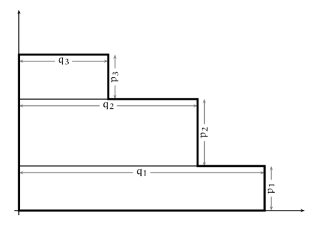
Figure 3. Generalized Young diagram $\mathbf{p}\times\mathbf{q}$ drawn in the French convention

If $\mathcal{F}:\mathbb{Y}\rightarrow\mathbb{R}$ is a sufficiently nice function on the set of generalized Young diagrams (in this article we use the class of, so called, polynomial functions) then $\mathcal{F}(\mathbf{p}\times\mathbf{q})$ turns out to be a polynomial in indeterminates $p_{1},p_{2},\dots,q_{1},q_{2},\dots$ which will be called Stanley polynomial. The Stanley polynomial for the most interesting functions $\mathcal{F}$, namely for the normalized characters $\Sigma_{\pi}$, is provided by Stanley-Féray character formula (Theorem 4.6) which was conjectured by Stanley [Sta06] and proved by Féray [Fér06], for a more elementary proof we refer to [FŚ07].

In the past analysis of some special coefficients of Stanley polynomials resulted in partial results concerning Kerov polynomials [Sta02, Sta04]. In Theorem 4.2 we will show that, in fact, a large class coefficients of Stanley polynomials can be interpreted as coefficients

$$\left.\frac{\partial}{\partial S_{k_{1}}}\cdots\frac{\partial}{\partial S_{k_{l}}}\mathcal{F}\right|_{S_{2}=S_{3}=\cdots=0}$$

in the Taylor expansion of $\mathcal{F}$ into the basic functionals $S_{2},S_{3},\dots$ of shape of a Young diagram.

These basic functionals $S_{2},S_{3},\dots$ of shape are not new; they already appeared (possibly with a slightly modified normalization) in the work of Ivanov and Olshanski [IO02] and implicitly in the work of Kerov [Ker98, Ker99, Ker03].

In this way we are able to express $\Sigma_{\pi}$ as an explicit polynomial in $S_{2},S_{3},\dots$. In Proposition 2.2 we will show how to express $S_{2},S_{3},\dots$ in terms of free cumulants $R_{2},R_{3},\dots$. Finally, we use some identities fulfilled by Stanley polynomials (Lemma 4.5) in order to express the coefficients of Kerov polynomials in a useful way.

1.8. Combinatorial interpretation of condition (e)

Let $(\sigma_{1},\sigma_{2},q)$ be a triple which fulfills conditions (a)–(d) of Theorem 1.4. We consider the following polyandrous interpretation of Hall marriage theorem. Each cycle of $\sigma_{1}$ will be called a boy and each cycle of $\sigma_{2}$ will be called a girl. For each girl $j\in C(\sigma_{2})$ let $q(j)-1$ be the desired number of husbands of $j$ (notice that condition (c) shows that the number of boys in $C(\sigma_{1})$ is right so that if no other restrictions were imposed it would be possible to arrange marriages in such a way that each boy is married to exactly one girl and each girl has the desired number of husbands). We say that a boy $i\in C(\sigma_{1})$ is a possible candidate for a husband for a girl $j\in C(\sigma_{2})$ if cycles $i$ and $j$ intersect. Hall marriage theorem applied to our setup says that there exists an arrangement of marriages $\mathcal{M}:C(\sigma_{1})\rightarrow C(\sigma_{2})$ which assigns to each boy his wife (so that each girl $j$ has exactly $q(j)-1$ husbands) if and only if for every set $A\subseteq C(\sigma_{2})$ there are at least $\sum_{i\in A}\big{(}q(i)-1\big{)}$ cycles of $\sigma_{1}$ which intersect $\bigcup A$. As one easily see, the above condition is similar but not identical to (e).

Proposition 1.7.

Condition (e) is equivalent to the following one:

1. for every nontrivial set of girls $A\subset C(\sigma_{2})$ (i.e., $A\neq\emptyset$ and $A\neq C(\sigma_{2})$) there exist two ways of arranging marriages $\mathcal{M}_{p}:C(\sigma_{1})\rightarrow C(\sigma_{2})$, $p\in\{1,2\}$ for which the corresponding sets of husbands of wives from $A$ are different:

   $$\mathcal{M}_{1}^{-1}(A)\neq\mathcal{M}_{2}^{-1}(A).$$

Proof.

The implication (e²)$\implies$(e) is immediate.

For the opposite implication Hall marriage theorem shows existence of $\mathcal{M}_{1}$. Let us select any boy $i\in\mathcal{M}_{1}^{-1}(A)$ and let us declare that boy $i$ is not allowed to marry any girl from the set $A$. Applying Hall marriage theorem for the second time shows existence of $\mathcal{M}_{2}$ with the required properties which finishes the proof of equivalence. ∎

For permutations $\sigma_{1},\sigma_{2}$ it is convenient to introduce a bipartite graph $\mathcal{V}^{\sigma_{1},\sigma_{2}}$ with the set of vertices $C(\sigma_{1})\sqcup C(\sigma_{2})$ with edges connecting intersecting cycles [FŚ07]. The elements of $C(\sigma_{1})$, respectively $C(\sigma_{2})$, will be referred to as white, respectively black, vertices. For a bipartite graph with a vertex set $V$ we will denote by $V_{\bullet}$ the set of black vertices.

The following result gives a strong restriction on the form of the factorizations which contribute to Theorem 1.4 and we hope it will be useful in the future investigations of Kerov polynomials. Notice that this kind of result appears also in the work of Féray [Fér09].

Proposition 1.8.

Suppose that $\sigma_{1},\sigma_{2}\in\mathfrak{S}(k)$ are such that in the graph $\mathcal{V}^{\sigma_{1},\sigma_{2}}$ there exists a disconnecting edge $e$ with a property that each of the two connected components of the resulting truncated graph $\mathcal{V}^{\sigma_{1},\sigma_{2}}\setminus\{e\}$ contains at least one vertex from $C(\sigma_{2})$. Then triple $(\sigma_{1},\sigma_{2},q)$ never contributes to the quantities described in Theorem 1.4 and Theorem 1.6, no matter how $q$ and $s_{2},s_{3},\dots$ are chosen.

Proof.

Before starting the proof notice that the assumptions of Theorem 1.4 and Theorem 1.6 show that in order for $(\sigma_{1},\sigma_{2},q)$ to contribute, graph $\mathcal{V}^{\sigma_{1},\sigma_{2}}$ must be connected.

Let $i\in C(\sigma_{1})$, $j\in C(\sigma_{2})$ be the endpoints of the edge $e$ and let $V_{1},V_{2}$ be the connected components of $\mathcal{V}^{\sigma_{1},\sigma_{2}}\setminus\{e\}$; we may assume that $i\in V_{1}$ and $j\in V_{2}$. We are going to use the condition (e²). Let $A$, respectively $B$, be the set of girls, respectively boys, contained in $V_{1}$. From the assumption it follows that $V_{1}\neq\{i\}$ therefore $A\neq\emptyset$; on the other hand $j\in V_{2}$ therefore $A\neq C(\sigma_{2})$.

If

(4) $$|B|-\sum_{j\in A}\big{(}q(j)-1\big{)}$$

does not belong to the set $\{0,1\}$ then it is not possible to arrange the marriages.

If (4) is equal to zero then any arrangement of marriages $\mathcal{M}:C(\sigma_{1})\rightarrow C(\sigma_{2})$ must fulfill $\mathcal{M}^{-1}(A)=B$; if (4) is equal to $1$ then any arrangement of marriages $\mathcal{M}:C(\sigma_{1})\rightarrow C(\sigma_{2})$ must fulfill $\mathcal{M}^{-1}(A)=B\setminus\{i\}$. In both cases, the set of husbands of wives from $A$ is uniquely determined therefore condition (e²) does not hold. ∎

1.9. Transportation interpretation of condition (e)

Let $G$ be a bipartite graph and its set of black vertices be $V_{\bullet}$. For any set $A\subseteq V_{\bullet}$ of black vertices we denote by $N_{G}(A)$ the set of white vertices which have a neighbor in $A$. We can rephrase condition (e) by:

1. for any non-trivial subset $A$, $\quad\left|N_{\mathcal{V}^{\sigma_{1},\sigma_{2}}}(A)\right|\geq 1+\sum_{c\in A}\big{[}q(c)-1\big{]}$.

Let a coloring $q:V_{\bullet}\rightarrow\{2,3,\dots\}$ of the black vertices of a bipartite graph $G$ be given. We say that $G$ is $q$-admissible if for every set $A\subseteq V_{\bullet}$ of black vertices $\left|N_{A}\right|\geq\sum_{c\in A}\big{[}q(c)-1\big{]}$ and furthermore the equality holds if and only if $V_{\bullet}$ is equal to the set of all black vertices in a union of some connected components of $G$.

Notice that if $G$ is connected then it is $q$-admissible if and only if it satisfies condition (e³).

Proposition 1.9.

Condition (e) is equivalent to the following one:

1. there exists a strictly positive solution to the following system of equations:

   Set of variables:

   $\big{\{}x_{i,j}:\text{ white vertex $i$ is connected to black vertex $j$}\big{\}}$

   Equations:

   $\left\{\begin{array}[]{l}\forall i,\sum_{j}x_{i,j}=1\\ \forall j,\sum_{i}x_{i,j}=q(j)-1\end{array}\right.$

More generally, graph $G$ is $q$-admissible if and only if condition (e⁴) is fulfilled.

Before starting the proof note that the possibility of arranging marriages (see Section 1.8) can be rephrased as existence of a solution to the above system of equations with a requirement that $x_{i,j}\in\{0,1\}$.

The system of equations in condition (e⁴) can be interpreted as a transportation problem where each white vertex is interpreted as a factory which produces a unit of some ware and each black vertex $j$ is interpreted as a consumer with a demand equal to $q(j)-1$. The value of $x_{i,j}$ is interpreted as amount of ware transported from factory $i$ to the consumer $j$.

Proof.

Suppose that the above system has a positive solution. For any $A\subseteq V_{\bullet}$ we have

$$\sum_{j\in A}(q(j)-1)=\sum_{j\in A}\sum_{\begin{subarray}{c}i:\\ (i,j)\text{ is an edge}\end{subarray}}x_{i,j}=\sum_{i\in N_{G}(A)}\sum_{\begin{subarray}{c}j\in A:\\ (i,j)\text{ is an edge}\end{subarray}}x_{i,j}\leq|N_{G}(A)|.$$

Furthermore, if $|N_{G}(A)|=\sum_{j\in A}(q(j)-1)$ then the above inequality is an equality which means that for each $i\in N_{G}(A)$ one has

$$\sum_{\begin{subarray}{c}j\in A:\\ (i,j)\text{ is an edge}\end{subarray}}x_{i,j}=1.$$

As $\sum\limits_{j}x_{i,j}=1$ and $x_{i,j}>0$ if $(i,j)$ is an edge, this implies that there is no edge $(i,j)$ with $i\in N_{G}(A)$ and $j\notin A$. In this way we have proved that $A$ is the set of black vertices of a union of some disjoint components, therefore $G$ is $q$-admissible.

The opposite implication is easy: we consider the mean of all solutions of the system with the condition $x_{i,j}\in\{0,1\}$. This gives us a strictly positive solution because the $q$-admissibility ensures that if we force some variable $x_{i,j}$ to be equal to $1$ we can find a solution to the system. ∎

1.10. Open problems

1.10.1. $C$-expansion

In analogy to (1) we define for $k\geq 2$

(5) $$C_{k}^{\lambda}=\frac{24}{k(k+1)(k+2)}\lim_{s\to\infty}\frac{1}{s^{k}}\left(\Sigma_{k+1}^{s\lambda}-R_{k+2}^{s\lambda}\right)$$

which (up to the unusual numerical factor in front) gives the leading terms of the deviation from the first-order approximation $\Sigma_{k+1}^{\lambda}\approx R_{k+2}^{\lambda}$. The explicit form of $C_{k}$

$$C_{k}=\sum_{\begin{subarray}{c}j_{2},j_{3},\dots\geq 0,\\ 2j_{2}+3j_{3}+\cdots=k\end{subarray}}\frac{(j_{2}+j_{3}+\cdots)!}{j_{2}!j_{3}!\cdots}\prod_{i\geq 2}\big{(}(i-1)R_{i})^{j_{i}}$$

as a polynomial in free cumulants $R_{2},R_{3},\dots$ was conjectured by Biane [Bia03] and was proved by Śniady [Śni06a]. Goulden and Rattan [GR07] proved that for each $k\geq 1$ there exists a universal polynomial $L_{k}$ called Goulden–Rattan polynomial with rational coefficients such that

(6) $$\Sigma_{k}-R_{k+1}=L_{k}(C_{2},C_{3},\dots)$$

and they found an explicit but complicated formula for $L_{k}$. A simpler proof and some more related results can be found in the work of Biane [Bia07].

Conjecture 1.10 (Goulden and Rattan [GR07]).

The coefficients of $L_{k}$ are non-negative rational numbers with relatively small denominators.

It is natural to conjecture that the underlying reason for positivity of the coefficients is that they have (after some additional rescaling) a combinatorial interpretation.

In some sense the free cumulants $(R_{k})$ are analogous to the above quantities $(C_{k})$: both have natural interpretations as leading (respectively, subleading) terms in the asymptotics of characters, cf. (1), respectively (5). Also, Conjecture 1.1 is analogous to Conjecture 1.10: both conjectures state that there are exact formulas which express the characters $\Sigma_{k}$ (respectively, the subdominant terms of the characters $\Sigma_{k}-R_{k+1}$) as polynomials in free cumulants (respectively, $(C_{k})_{k\geq 2}$) with non-negative integer coefficients (respectively, non-negative rational coefficients with small denominators) which have a combinatorial interpretation.

The advantage of the quantities $(C_{k})$ over free cumulants $(R_{k})$ is that the Goulden–Rattan polynomials $L_{k}$ seem to have a simpler form than Kerov polynomials $K_{k}$ while the numerical evidence for Conjecture 1.10 suggests that their coefficients should have a rich and beautiful structure. Also, Kerov’s conjecture (Conjecture 1.1) would be an immediate corollary from Conjecture 1.10. For these reasons we tend to believe that the quantities $(C_{k})$ are even better suitable for the asymptotic representation theory then the free cumulants $(R_{k})$ and Conjecture 1.10 deserves serious interest.

1.10.2. $\mathcal{R}$-expansion

Another interesting direction of research was pointed out by Lassalle [Las08] who presented quite explicit conjectures on the form of the coefficients of Kerov polynomials.

1.10.3. Arithmetic properties of Kerov polynomials

Proposition 1.11.

If $p$ is an odd prime number then $\frac{\Sigma_{p}-R_{p+1}+2R_{2}}{p}$ and $\frac{\Sigma_{p-1}-R_{p}}{p}$ are polynomials in free cumulants $R_{2},R_{3},\dots$ with nonnegative integer coefficients.

Proof.

In order to prove that the coefficients of $\frac{\Sigma_{p}-R_{p+1}+2R_{2}}{p}$ are integer we consider the action of the group $\mathbb{Z}/p\mathbb{Z}$ on the set of triples $(\sigma_{1},\sigma_{2},q)$ which contribute to Theorem 1.4 defined by conjugation

$$\psi(i)(\sigma_{1},\sigma_{2},q)=\big{(}c^{i}\sigma_{1}c^{-i},c^{i}\sigma_{2}c^{-i},q^{\prime}),$$

where $c=(1,2,\dots,k)$ is the cycle; we leave the details how to define $q^{\prime}$ as a simple exercise. All orbits of this action consist of $p$ elements except for the fixpoints of this action which are of the form $\sigma_{1}=c^{a}$, $\sigma_{2}=c^{1-a}$. These fixpoints contribute to the monomial $R_{k+1}$ (with multiplicity $1$) and to the monomial $R_{2}$ (with multiplicity $p-2$).

In order to prove that the coefficients of $\frac{\Sigma_{p-1}-R_{p}}{p}$ are integer we express $R_{p}$ as a linear combination of the conjugacy classes $\Sigma_{\pi}$. A formula for such an expansion presented in the paper [Śni06a] involves summation over all partitions of the set $\{1,\dots,p\}$. The group $\mathbb{Z}/p\mathbb{Z}$ acts on such partitions; all orbits in this action consist of $p$ elements except for the fixpoints of this action: the minimal partition (which gives $\Sigma_{p-1}$) and the maximal partition (which turns out not to contribute). We express all summands (except for the summand corresponding to $\Sigma_{p-1}$) as polynomials in free cumulants, which finishes the proof. ∎

The following conjecture was formulated by Światosław Gal (private communication) based on numerical calculations.

Conjecture 1.12.

If $p$ is an odd prime number then and $\frac{\Sigma_{p+1}-R_{p+2}+R_{3}}{p}$ is a polynomial in free cumulants $R_{2},R_{3},\dots$ with nonnegative integer coefficients.

We hope that the above claims will shed some light on more precise structure of Kerov polynomials and on the form of $C$-expansion and $\mathcal{R}$-expansion described above; they suggest that (maybe up to some small error terms) $\Sigma_{n}-R_{n+1}$ should in some sense be divisible by $(n-1)n(n+1)$ which supports the conjectures of Lassalle [Las08].

1.10.4. Discrete version of the functionals $S_{2},S_{3},\dots$

One of the fundamental ideas in this paper is the use of the fundamental functionals $S_{2},S_{3},\dots$ of the shape of a Young diagram defined as integrals over the area of a Young diagram of the powers of the contents:

(7) $$S^{\lambda}_{n}=(n-1)\iint_{\Box\in\lambda}(\operatorname{contents}_{\Box})^{n-2}\ d\Box$$

(we postpone the precise definition until Section 3.2).

It would be interesting to investigate properties of analogous quantities

(8) $$T^{\lambda}_{n}=(n-1)\sum_{\Box\in\lambda}(\operatorname{contents}_{\Box})^{n-2}$$

in which the integral over the Young diagram was replaced by a sum over its boxes. Notice that unlike the integrals (7) which are well-defined for generalized Young diagrams, the sum (8) makes sense only if $\lambda$ is a conventional Young diagram but since the resulting object is a polynomial function on the set of Young diagrams it can be extended to generalized Young diagrams. This type of quantities have been investigated by Corteel, Goupil and Schaeffer [CGS04].

The reason why we find the functional $T_{n}$ so interesting is that via non-commutative Fourier transform it corresponds to a central element of the symmetric group algebra $\mathbb{C}[\mathfrak{S}(k)]$ given by the following very simple formula

$$T_{n}=(n-1)\sum_{2\leq i\leq n}X_{i}^{n-2},$$

where

$$X_{i}=(1,i)+(2,i)+\cdots+(i-1,i)\in\mathbb{C}[\mathfrak{S}(k)]$$

are the Jucys-Murphy elements.

The hidden underlying idea behind the current paper is the differential calculus on the (polynomial) functions on the set of generalized Young diagrams $\mathbb{Y}$ in which we study derivatives corresponding to infinitesimal changes of the shape of a Young diagram, as it can be seen in the proof of Theorem 4.2. It is possible to develop the formalism of such a differential calculus and to express the results of this paper in such a language instead of the language of Stanley polynomials (and, in fact, the initial version of this article was formulated in this way), nevertheless if the main goal is to prove the Kerov conjecture then this would lead to unnecessary complication of the paper.

On the other hand, just like the usual differential and integral calculus has an interesting discrete difference and sum analogue, the above described differential calculus on generalized Young diagrams has a discrete difference analogue in which we study the change of the function on the set of Young diagrams corresponding to addition or removal of a single box. We expect that just like functionals $(S_{n})$ are so useful in the framework of differential calculus on the set of generalized Young diagrams, functionals $(T_{n})$ will be useful in the framework of the difference calculus on Young diagrams.

It would be very interesting to develop such a difference calculus and to verify if free cumulants $(R_{n})$ have some interesting discrete version which nicely fits into this setup.

1.10.5. Characterization of Stanley polynomials

Lemma 4.5 contains some identities fulfilled by Stanley polynomials. It would be interesting to find some more such identities. In particular we state the following problem here.

Problem 1.13.

Find (minimal set of) conditions which fully characterize the class of Stanley polynomials $\mathcal{F}(\mathbf{p}\times\mathbf{q})$ where $\mathcal{F}$ is a polynomial function on the set of Young diagrams.

It seems plausible that the answer for this problem is best formulated in the language of the differential calculus of function on the set of generalized Young diagrams about which we mentioned in Section 1.10.4.

1.10.6. Various open problems

Is there some analogue of Kerov character polynomials for the representation theory of semisimple Lie groups, in particular for the unitary groups $U(d)$? Does existence of Kerov polynomials for characters of symmetric groups $\mathfrak{S}(n)$ tell us something (for example via Schur-Weyl duality) about representations of the unitary groups $U(d)$? Is there some analogue of Kerov character polynomials in the random matrix theory? Is it possible to study Kerov polynomials in such a scaling that phenomena of universality of random matrices occur?

1.11. Exotic interpretations of Kerov polynomials

Theorem 1.4 gives some interpretation of the coefficients of Kerov polynomials but clearly it does not mean that there are no other interpretations.

1.11.1. Biane’s decomposition

The original conjecture of Biane [Bia03] suggested that the coefficients of Kerov polynomials are equal to multiplicities in some unspecified decomposition of the Cayley graph of the symmetric group into a signed sum of non-crossing partitions. This result was proved by Féray [Fér09] but the details of his construction were quite implicit. In Section 8 we shall revisit the conjecture of Biane in the light of our new combinatorial interpretation of Kerov polynomials. Unfortunately, our understanding of this interpretation of the coefficients of Kerov polynomials is still not satisfactory and remains as an open problem.

1.11.2. Multirectangular random matrices

For a given Young diagram $\lambda$ we consider a Gaussian random matrix $(A^{\lambda}_{ij})$ with the shape of $\lambda$. Formally speaking, the entries of $(A^{\lambda}_{ij})$ are independent with $A^{\lambda}_{ij}=0$ if box $(i,j)$ does not belong to $\lambda$; otherwise $\Re A^{\lambda}_{ij},\Im A^{\lambda}_{ij}$ are independent Gaussian random variables with mean zero and variance $\frac{1}{2}$. One can think that either $(A^{\lambda}_{ij})$ is an infinite matrix or it is a square (or rectangular) matrix of sufficiently big size.

Theorem 1.14.

Kerov polynomials express the moments of the random matrix $A^{\lambda}$ in terms of the genus-zero terms in the genus expansion (up to the sign). More precisely,

$$\mathbb{E}\left[\operatorname{Tr}\big{(}A^{\lambda}(A^{\lambda}{})^{\star}\big{)}^{n}\right]=-K_{n}(-R_{2},-R_{3},-R_{4},\dots),$$

where $R_{i}$ is defined as the genus zero term in the expansion for

$$\mathbb{E}\left[\operatorname{Tr}\left(A^{\lambda}\left(A^{\lambda}\right)^{\star}\right)^{i-1}\right],$$

or, precisely speaking,

$$R_{i}=\lim_{s\to\infty}\frac{1}{s^{i}}\mathbb{E}\left[\operatorname{Tr}\left(A^{s\lambda}\left(A^{s\lambda}\right)^{\star}\right)^{i-1}\right].$$

This is an immediate consequence of the results from [FŚ07].

1.11.3. Dimensions of (co)homologies

In analogy to Kazhdan-Lusztig polynomials it is tempting to ask if the coefficients of Kerov polynomials might have a topological interpretation, for example as dimensions of (co)homologies of some interesting geometric objects, maybe related to Schubert varieties, as suggested by Biane (private communication). This would be supported by the Biane’s decomposition from Section 1.11.1 which maybe is related to Bruhat order and Schubert cells. In this context it is interesting to ask if the conditions from Theorem 1.4 can be interpreted as geometric conditions on intersections of some geometric objects. Another approach towards establishing link between Kerov polynomials and Schubert calculus would be to relate Kerov polynomials and Schur symmetric polynomials.

1.11.4. Schur polynomials

Each Schur polynomial can be written as quotient of two determinants. Exactly the same quotient of determinants appears in the Harish-Chandra-Itzykson-Zuber integral

$$\int_{U(d)}e^{AUBU^{\star}}dU$$

if $A$ and $B$ are hermitian matrices with suitably chosen eigenvalues (say $(x_{i})$ for $A$ and $(\log\lambda_{i})$ for $B$).

It would be interesting to verify if Kerov polynomials can be used to express the exact values of Schur polynomials by some limit value of Harish-Chandra-Itzykson-Zuber integral when the size of the matrix tends to infinity and each variable $x_{i}$ occurs with a multiplicity which tends to infinity; also the shape of the Young diagram $\lambda$ should tend to infinity, probably in the “balanced Young diagram” way.

1.11.5. Analytic maps

We conjecture that Kerov polynomials are related to moduli space of analytic maps on Riemann surfaces or ramified coverings of a sphere.

1.11.6. Integrable hierarchy

Jonathan Novak (private communication) conjectured that Kerov polynomials might be algebraic solutions to some integrable hierarchy (maybe Toda?) and their coefficients are related to the tau function of the hierarchy.

1.12. Applications of the main result

1.12.1. Positivity conjectures and precise information on Kerov polynomials

The advantage of the approach to characters of symmetric groups presented in this article over some other methods is that the formula for the coefficients given by Theorem 1.4 does not involve summation of terms of positive and negative sign unlike most formulas for characters such as Murnaghan-Nakayama rule or Stanley-Féray formula (Theorem 4.6). In this way we avoid dealing with complicated cancellations. For this reason the main result of the current paper seems to be a perfect tool for proving stronger results, such as the Conjecture 1.10 of Goulden and Rattan or the conjectures of Lassalle [Las08].

1.12.2. Genus expansion

One of the important methods in the random matrix theory and in the representation theory is to express the quantity we are interested in (for example: moment of a random matrix or character of a representation) as a sum indexed by some combinatorial objects (for example: partitions of an ordered set or maps) to which one can associate canonically a two-dimensional surface [LZ04]. Usually the asymptotic contribution of such a summand depends on the topology of the surface with planar objects being asymptotically dominant. This method is called genus expansion since exponent describing the rate of decay of a given term usually linearly depends on the genus.

The main result of this article fits perfectly into this philosophy since to any pair of permutations $\sigma_{1}$, $\sigma_{2}$ which contributes to Theorem 1.4 or Theorem 1.6 we may associate a canonical graph on a surface, called a map. It is not difficult to show that also in this situation the degree of the terms $R_{2}^{s_{2}}R_{3}^{s_{3}}\cdots$ to which such a pair of permutations contributes decreases as the genus increases.

It is natural therefore to ask about the structure of factorizations $\sigma_{1}\circ\sigma_{2}=(1,2,\dots,k)$ with a prescribed genus. As we already pointed out in Proposition 1.8, condition (e) of Theorem 1.4 gives strong limitations on the shape of the resulting bipartite graph $\mathcal{V}^{\sigma_{1},\sigma_{2}}$ which translate to limitations on the shape of the corresponding map. Very analogous situation was analyzed in the paper [Śni06a] where it was proved that by combining a restriction on the genus and a condition analogous to the one from Proposition 1.8 (“evercrossing partitions”) one gets only a finite number of allowed patterns for the geometric object concerned.

Similar analysis should be possible for the formulas for Kerov polynomials presented in the current paper which should shed some light on Conjecture 1.10 of Goulden and Rattan and the conjectures of Lassalle [Las08].

1.12.3. Upper bounds on characters

It seems plausible that the main result of this article, Theorem 1.4 and Theorem 1.6, can be used to prove new upper bounds on the characters of symmetric groups

(9) $$\chi^{\lambda}(\pi)=\frac{\operatorname{Tr}\rho^{\lambda}(\pi)}{\text{dimension of $\rho^{\lambda}$}}$$

for balanced Young diagram $\lambda$ in the scaling when the length of the permutation $\pi$ is large compared to the number of boxes of $\lambda$.

The advantage of such approach to estimates on characters over other methods, such as via Frobenius formula as in the work of Rattan and Śniady [RŚ08] or via Stanley-Féray formula [FŚ07], becomes particularly visible in the case when the shape of the Young diagram becomes close to the limit curve for the Plancherel measure [LS77, VK77] for which all free cumulants (except for $R_{2}$) are close to zero. Indeed, for $\lambda$ in the neighborhood of this limit curve one should expect much tighter bounds on the characters (9) because such Young diagrams maximize the dimension of the representation which is the denominator of the fraction, while the numerator can be estimated by Murnaghan-Nakayama rule and some combinatorial tricks [Roi96].

1.13. Overview of the paper

In Section 2 we recall some basic facts about free cumulants $R_{1},R_{2},\dots$ and quantities $S_{1},S_{2},\dots$ for probability measures on the real line and their relations with each other. The main result of this section is formula (14) which allows to express functionals $S_{1},S_{2},\dots$ in terms of free cumulants $R_{1},R_{2},\dots$.

In Section 3 we define the fundamental functionals $S_{2},S_{3},\dots$ for generalized Young diagrams and study their geometric interpretation.

In Section 4 we study Stanley polynomials and their relations to the fundamental functionals $S_{2},S_{3},\dots$ of shape of a Young diagram.

Section 5 is devoted to a toy example: we shall prove Theorem 1.4 in the simplest non-trivial case of coefficients of the quadratic terms, which is exactly the case in Theorem 1.3. In this way the Reader can see all essential steps of the proof in a simplified situation when it is possible to avoid technical difficulties.

In Section 6 we prove some auxiliary combinatorial results.

In Section 7 we present the proof of the main result: Theorem 1.4 and Theorem 1.6.

Finally, in Section 8 we revisit the paper [Fér09] and we show how rather implicit constructions of Féray become much more concrete once one knows the formulation of the main result of the current paper, Theorem 1.4. In fact, Section 8 provides a short proof of Theorem 1.4 based on results from of Féray. This simplicity is however slightly misleading since the original paper [Fér09] is not easy.

2. Functionals of measures

In this section we present relations between moments $M_{1},M_{2},\dots$ of a given probability measure, its free cumulants $R_{1},R_{2},\dots$ and its functionals $S_{1},S_{2},\dots$. The only result of this section which will be used in the remaining part of the article is equality (14), nevertheless we find functionals $S_{1},S_{2},\dots$ so important that we collected in this section also some other formulas involving them.

Assume that $\nu$ is a compactly supported measure on $\mathbb{R}$. For integer $n\geq 0$ we consider moments of $\nu$

$$M^{\nu}_{n}=\int z^{n}d\nu(z)$$

and its Cauchy transform

$$G^{\nu}(z)=\int\frac{1}{z-x}d\nu(x)=\sum_{n\geq 0}\frac{M_{n}^{\nu}}{z^{1+n}};$$

the integral and the series make sense in a neighborhood of infinity.

From the following on we assume that $\nu$ is a compactly supported probability measure on $\mathbb{R}$. We define a sequence $(S^{\nu}_{n})_{n\geq 1}$ of the coefficients of the expansion

$$S^{\nu}(z)=\log zG^{\nu}(z)=\sum_{n\geq 1}\frac{S^{\nu}_{n}}{z^{n}}$$

in a neighborhood of infinity and a sequence $(R^{\nu}_{n})_{n\geq 1}$ of free cumulants as the coefficients of the expansion

(10) $$R^{\nu}(z)=\left(G^{\nu}\right)^{\langle-1\rangle}(z)-\frac{1}{z}=\sum_{n\geq 1}R^{\nu}_{n}z^{n-1}$$

in a neighborhood of $0$, where $\left(G^{\nu}\right)^{\langle-1\rangle}$ is the right inverse of $G^{\nu}$ with respect to the composition of functions [Voi86]. When it does not lead to confusions we shall omit the superscript in the expressions $M^{\nu}_{n}$, $G^{\nu}$, $S^{\nu}$, $R^{\nu}$, $S^{\nu}_{n}$, $R^{\nu}_{n}$.

The relation between the moments and the free cumulants is given by the following combinatorial formula which, in fact, can be regarded as an alternative definition of free cumulants [Spe98]:

(11) $$M_{n}=\sum_{\Pi\in\operatorname{NC}_{n}}R_{\Pi},$$

where the summation is carried over all non-crossing partitions of $n$-element set and where $R_{\Pi}$ is defined as the multiplicative extension of $(R_{k})$:

$$R_{\Pi}=\prod_{b\in\Pi}R_{|b|},$$

where the product is taken over all blocks $b$ of the partition $\Pi$ and $|b|$ denotes the number of the elements in $b$ [Spe98].

Information about the measure $\nu$ can be described in various ways; in this article descriptions in terms of the sequences $(S_{n})$ and $(R_{n})$ play eminent role and we need to be able to relate each of these sequences to the other. We shall do it in the following.

Lemma 2.1.

For any integer $k\geq 1$

$$\frac{\partial G(R_{1},R_{2},\dots)}{\partial R_{k}}(z)=-\frac{1}{k}\bigg{(}\big{[}G(z)\big{]}^{k}\bigg{)}^{\prime}=-G^{k-1}(z)G^{\prime}(z),$$

where both sides of the above equality are regarded as formal power series in powers of $\frac{1}{z}$ with the coefficients being polynomials in $R_{1},R_{2},\dots$.

Proof.

Equation (10) is equivalent to

(12) $$G\left(R(z)+\frac{1}{z}\right)=z.$$

We denote

$$t=R(z)+\frac{1}{z}.$$

Let us keep all free cumulants fixed except for $R_{k}$, we shall treat $G$ as a function of free cumulants. By taking the derivatives of both sides of (12) it follows that

$$0=\frac{\partial}{\partial R_{k}}\left[G\left(R(z)+\frac{1}{z}\right)\right]=\frac{\partial G}{\partial R_{k}}(t)+G^{\prime}(t)\frac{\partial}{\partial R_{k}}\left(R(z)+\frac{1}{z}\right)=\\ \frac{\partial G}{\partial R_{k}}(t)+G^{\prime}(t)z^{k-1}=\frac{\partial G}{\partial R_{k}}(t)+G^{\prime}(t)\cdot G^{k-1}(t)$$

which finishes the proof. ∎

Proposition 2.2.

For any integer $n\geq 1$

(13) $$M_{n} =\sum_{l\geq 1}\frac{1}{l!}(n)_{l-1}\sum_{\begin{subarray}{c}k_{1},\dots,k_{l}\geq 1\\ k_{1}+\cdots+k_{l}=n\end{subarray}}R_{k_{1}}\cdots R_{k_{l}},$$

(14) $$S_{n} =\sum_{l\geq 1}\frac{1}{l!}(n-1)_{l-1}\sum_{\begin{subarray}{c}k_{1},\dots,k_{l}\geq 1\\ k_{1}+\cdots+k_{l}=n\end{subarray}}R_{k_{1}}\cdots R_{k_{l}},$$

(15) $$R_{n} =\sum_{l\geq 1}\frac{1}{l!}(-n+1)^{l-1}\sum_{\begin{subarray}{c}k_{1},\dots,k_{l}\geq 1\\ k_{1}+\cdots+k_{l}=n\end{subarray}}S_{k_{1}}\cdots S_{k_{l}},$$

where

$$(a)_{b}=\underbrace{a(a-1)\cdots(a-b+1)}_{b\text{ factors}}$$

denotes the falling factorial.

Proof.

Lemma 2.1 shows that

$$\frac{\partial^{2}G(R_{1},R_{2},\dots)}{\partial R_{k}\ \partial R_{l}}(z)=\frac{1}{k+l-1}\bigg{(}\big{[}G(z)\big{]}^{k+l-1}\bigg{)}^{\prime\prime}$$

therefore if $k+l=k^{\prime}+l^{\prime}$ then

$$\frac{\partial^{2}M_{n}(R_{1},R_{2},\dots)}{\partial R_{k}\ \partial R_{l}}=\frac{\partial^{2}M_{n}(R_{1},R_{2},\dots)}{\partial R_{k^{\prime}}\ \partial R_{l^{\prime}}}.$$

It follows by induction that

$$\frac{\partial^{l}M_{n}(R_{1},R_{2},\dots)}{\partial R_{k_{1}}\cdots\partial R_{k_{l}}}=\frac{\partial^{l}M_{n}(R_{1},R_{2},\dots)}{(\partial R_{1})^{l-1}\partial R_{k_{1}+\cdots+k_{l}-(l-1)}}.$$

From the moment-cumulant formula (11) it follows that for $R_{1}=R_{2}=\cdots=0$ the right-hand side of the above equation is equal to the number of non-crossing partitions with an ordering of blocks, such that the numbers of elements in consecutive blocks are as follows:

$$\underbrace{1,\dots,1}_{l-1\text{ times}},k_{1}+\cdots+k_{l}-(l-1).$$

Such non-crossing partitions have a particularly simple structure therefore it is very easy to find their cardinality. Therefore

(16) $$\left.\frac{\partial^{l}M_{n}(R_{1},R_{2},\dots)}{(\partial R_{1})^{l-1}\partial R_{k_{1}+\cdots+k_{l}-(l-1)}}\right|_{R_{1}=R_{2}=\cdots=0}=\begin{cases}(n)_{l-1}&\text{if }n=k_{1}+\cdots+k_{l},\\ 0&\text{otherwise,}\end{cases}$$

which finishes the proof of (13).

Lemma 2.1 shows that for $k\geq 2$

$$\frac{\partial S(R_{1},R_{2},\dots)}{\partial R_{k}}(z)=\frac{\partial\log\big{[}zG(z)\big{]}}{\partial R_{k}}=-G^{k-2}G^{\prime}=\frac{\partial G(R_{1},R_{2},\dots)}{\partial R_{k-1}}$$

therefore

$$\frac{\partial S_{n}(R_{1},R_{2},\dots)}{\partial R_{k}}=\frac{\partial M_{n-1}(R_{1},R_{2},\dots)}{\partial R_{k-1}}.$$

Assume that $k_{l}\geq 2$; then

$$\frac{\partial^{l}S_{n}(R_{1},R_{2},\dots)}{\partial R_{k_{1}}\cdots\partial R_{k_{l}}}=\frac{\partial^{l}M_{n-1}(R_{1},R_{2},\dots)}{\partial R_{k_{1}}\cdots\partial R_{k_{l}-1}}$$

which is calculated in Eq. (16). In this way we proved that if $(k_{1},\dots,k_{l})\neq(1,1,\cdots,1)$ then

$$\left.\frac{\partial^{l}S_{n}(R_{1},R_{2},\dots)}{\partial R_{k_{1}}\cdots\partial R_{k_{l}}}\right|_{R_{1}=R_{2}=\cdots=0}=\begin{cases}(n-1)_{l-1}&\text{if }n=k_{1}+\cdots+k_{l},\\ 0&\text{otherwise.}\end{cases}$$

In order to prove the case $k_{1}=\cdots=k_{l}=1$ it is enough to consider the Dirac point measure $\nu=\delta_{a}$ for which $G(z)=\frac{1}{z-a}$, $R_{1}=a$, $R_{2}=R_{3}=\cdots=0$ and $S(z)=-\log\left(1-\frac{a}{z}\right)$, $S_{n}=\frac{a^{n}}{n}$. In this way the proof of (14) is finished.

Lagrange inversion formula shows that

$$R_{n+1}=-\frac{1}{n}\left[\frac{1}{z}\right]\left(\frac{1}{G(z)}\right)^{n}=-\frac{1}{n}\left[\frac{1}{z^{n+1}}\right]\exp[-nS(z)]=\\ \sum_{l\geq 1}\frac{1}{l!}(-n)^{l-1}\sum_{\begin{subarray}{c}k_{1},\dots,k_{l}\geq 1\\ k_{1}+\cdots+k_{l}=n+1\end{subarray}}S_{k_{1}}\cdots S_{k_{l}}$$

which finishes the proof of (15). ∎

3. Generalized Young diagrams

The main result of this section is the formula (17) which relates the fundamental functionals $S_{2},S_{3},\dots$ to the geometric shape of the Young diagram.

In the following we base on the notations introduced in Section 1.1.

3.1. Measure on a diagram and contents of a box

Notice that each unit box of a Young diagram drawn in the French convention becomes in the Russian notation a square of side $\sqrt{2}$. For this reason, when drawing a Young diagram according to the French convention we will use the plane equipped with the usual measure (i.e. the area of a unit square is equal to $1$) and when drawing a Young diagram according to the Russian notation we will use the plane equipped with the usual measure divided by $2$ (i.e. the area of a unit square is equal to $\frac{1}{2}$). In this way a (generalized) Young diagram has the same area when drawn in the French and in the Russian convention.

Speaking very informally, the setup of generalized Young diagrams corresponds to looking at a Young diagram from very far away so that individual boxes become very small. Therefore by the term box of a Young diagram $\lambda$ we will understand simply any point $\Box$ which belongs to $\lambda$. In the case of the Russian convention this means that $\Box=(x,y)$ fulfills

$$|x|<y<\lambda(x).$$

We define the contents of the box $\Box=(x,y)$ in the Russian convention by $\operatorname{contents}_{\Box}=x$.

In the case of the French convention $\Box=(x,y)$ belongs to a diagram $\lambda$ if

$$x>0\qquad\text{ and }\qquad 0<y<\lambda(x)$$

and the contents of the box $\Box=(x,y)$ is defined by $\operatorname{contents}_{\Box}=x-y$.

3.2. Functionals of Young diagrams

The above definitions of the measure on the plane and of the contents in the case of French and Russian conventions are compatible with each other, therefore it is possible to define some quantities in a convention-independent way. In particular, we define the fundamental functionals of shape of a generalized Young diagram

(17) $$S^{\lambda}_{n}=(n-1)\iint_{\Box\in\lambda}(\operatorname{contents}_{\Box})^{n-2}\ d\Box$$

for integer $n\geq 2$. Clearly, each functional $S_{n}$ is a homogeneous function of the Young diagram with degree $n$.

Let a generalized Young diagram $\lambda:\mathbb{R}\rightarrow\mathbb{R}_{+}$ drawn in the Russian convention be fixed. We associate to it a function

$$\tau^{\lambda}(x)=\frac{\lambda(x)-|x|}{2}$$

which gives the distribution of the contents of the boxes of $\lambda$. When it does not lead to confusions we will write for simplicity $\tau$ instead of $\tau^{\lambda}$. In the following we shall view $\tau$ as a measure on $\mathbb{R}$. Its Cauchy transform can be written as

$$G^{\tau}(z)=\iint_{\Box\in\lambda}\frac{1}{z-\operatorname{contents}_{\Box}}d\Box.$$

With these notations we have that

$$S^{\lambda}_{n}=(n-1)\int x^{n-2}\ \tau(x)\ dx=-\int x^{n-1}\ \tau^{\prime}(x)\ dx$$

are (rescaled) moments of the measure $\tau$ or, alternatively, (shifted) moments of the Schwartz distribution $-\tau^{\prime}$.

We define

$$S^{\lambda}(z)=\sum_{n\geq 2}\frac{S^{\lambda}_{n}}{z^{n}}=\iint_{\Box\in\lambda}\frac{1}{(z-\operatorname{contents}_{\Box})^{2}}\ d\Box$$

where the second equality follows by expanding right-hand side into a power series and (17). It follows that

$$S^{\lambda}(z)=-\frac{d}{dz}G^{\tau}(z)=G^{-\tau^{\prime}}(z)=-\int\frac{1}{z-x}\tau^{\prime}(x)\ dx=\\ -\int\log(z-x)\ \tau^{\prime\prime}(x)\ dx,$$

in particular $S^{\lambda}(z)$ coincides with the Cauchy transform of a Schwartz distribution $-\tau^{\prime}$. The above formulas show that $S^{\lambda}(z)$ and $S_{n}^{\lambda}(z)$ coincide (up to small modifications) with the quantities considered by Kerov [Ker99, Ker03], Ivanov and Olshanski [IO02].

3.3. Kerov transition measure

The corresponding Cauchy transform

(18) $$G^{\lambda}(z)=\frac{1}{z}\exp S^{\lambda}(z)$$

is a Cauchy transform of a probability measure $\mu_{\lambda}$ on the real line, called Kerov transition measure of $\lambda$ [Ker99, Ker03]. Probably it would be more correct to write $G^{\mu_{\lambda}}$ instead of $G^{\lambda}$ and to write $S^{\mu_{\lambda}}$ instead of $S^{\lambda}$, but this would lead to unnecessary complexity of the notation.

One of the reasons why Kerov’s transition measure was so successful in the asymptotic representation theory of symmetric groups is that it can be defined in several equivalent ways, related either to the shape of $\lambda$ or to representation theory or to moments of Jucys-Murphy elements or to certain matrices. For a review of these approaches we refer to [Bia98].

3.4. Free cumulants of a Young diagram

In order to keep the introduction as non-technical as possible, we introduced free cumulants of a Young diagram by the formula (1). The conventional way of defining them is to use (10) for the Cauchy transform given by (18). Therefore, one should make sure that these two definitions are equivalent. This can be done thanks to Frobenius formula

$$\Sigma_{k-1}^{\lambda}=-\frac{1}{k-1}\left[\frac{1}{z}\right]\frac{1}{G^{\lambda}(z-1)G^{\lambda}(z-2)\cdots G^{\lambda}\big{(}z-(k-1)\big{)}}$$

which shows that

$$\frac{1}{s^{k}}\Sigma_{k-1}^{s\lambda}=-\frac{1}{k-1}\left[\frac{1}{z}\right]\frac{1}{G^{\lambda}\left(z-\frac{1}{s}\right)G^{\lambda}\left(z-\frac{2}{s}\right)\cdots G^{\lambda}\left(z-\frac{k-1}{s}\right)};$$

therefore definition (1) would give

$$R^{\lambda}_{k}=-\frac{1}{k-1}\left[\frac{1}{z}\right]\left(\frac{1}{G^{\lambda}(z)}\right)^{k-1}$$

which coincides with the value given by the Lagrange inversion formula applied to (10).

3.5. Polynomial functions on the set of Young diagrams

For simplicity we shall often drop the explicit dependence of the functionals of Young diagrams from $\lambda$. Since the transition measure $\mu^{\lambda}$ is always centered it follows that $M_{1}=R_{1}=S_{1}=0$.

Existence of Kerov polynomials allows us define formally the normalized characters $\Sigma_{\pi}^{\lambda}$ even if $\lambda$ is a generalized Young diagram.

We will say that a function on the set of generalized Young diagrams $\mathbb{Y}$ is a polynomial function if one of the following equivalent conditions hold [IO02]:

• it is a polynomial in $M_{2},M_{3},\dots$;

• it is a polynomial in $S_{2},S_{3},\dots$;

• it is a polynomial in $R_{2},R_{3},\dots$;

• it is a polynomial in $(\Sigma_{\pi})_{\pi}$.

4. Stanley polynomials and Stanley-Féray character formula

4.1. Stanley polynomials

Proposition 4.1.

Let $\mathcal{F}:\mathbb{Y}\rightarrow\mathbb{R}$ be a polynomial function on the set of generalized Young diagrams. Then $(\mathbf{p},\mathbf{q})\mapsto\mathcal{F}(\mathbf{p}\times\mathbf{q})$ for $\mathbf{p}=(p_{1},\dots,p_{m})$, $\mathbf{q}=(q_{1},\dots,q_{m})$ is a polynomial in indeterminates $p_{1},\dots,p_{m},q_{1},\dots,q_{m}$, called Stanley polynomial.

Proof.

It is enough to prove this proposition for some family of generators of the algebra of polynomial functions on $\mathbb{Y}$ for example for functionals $S_{2},S_{3},\dots$. We leave it as an exercise. ∎

Theorem 4.2.

Let $\mathcal{F}:\mathbb{Y}\rightarrow\mathbb{R}$ be a polynomial function on the set of generalized Young diagrams, we shall view it as a polynomial in $S_{2},S_{3},\dots$ Then for any $k_{1},\dots,k_{l}\geq 2$

(19) $$\left.\frac{\partial}{\partial S_{k_{1}}}\cdots\frac{\partial}{\partial S_{k_{l}}}\mathcal{F}\right|_{S_{2}=S_{3}=\cdots=0}=[p_{1}q_{1}^{k_{1}-1}\cdots p_{l}q_{l}^{k_{l}-1}]\mathcal{F}(\mathbf{p}\times\mathbf{q}).$$

Proof.

Let $\mathbf{p}=(p_{1},\dots,p_{m})$, $\mathbf{q}=(q_{1},\dots,q_{m})$. For a given index $i$ we consider a trajectory in the set of generalized Young diagrams $q_{i}\mapsto(\mathbf{p}\times\mathbf{q})$, where all other parameters $(p_{j})$ and $(q_{j})_{j\neq i}$ are treated as constants. In the Russian convention we have

$$\left(\frac{\partial}{\partial q_{i}}(\mathbf{p}\times\mathbf{q})\right)(x)=\\ \begin{cases}2&\text{if }q_{i}-p_{1}-\cdots-p_{i}<x<q_{i}-p_{1}-\cdots-p_{i-1},\\ 0&\text{otherwise},\end{cases}$$

which shows the change of the contents distribution. From (17) it follows therefore

$$\frac{\partial}{\partial q_{i}}S_{n}^{\mathbf{p}\times\mathbf{q}}=\int_{q_{i}-p_{1}-\cdots-p_{i}}^{q_{i}-p_{1}-\cdots-p_{i-1}}\ (n-1)x^{n-2}\ dx$$

and

$$\frac{\partial}{\partial q_{i}}\mathcal{F}(\mathbf{p}\times\mathbf{q})=\sum_{n\geq 2}\int_{q_{i}-p_{1}-\cdots-p_{i}}^{q_{i}-p_{1}-\cdots-p_{i-1}}\frac{\partial\mathcal{F}}{\partial S_{n}}\ (n-1)x^{n-2}\ dx.$$

By iterating the above argument we show that

$$\frac{\partial}{\partial q_{1}}\cdots\frac{\partial}{\partial q_{l}}\mathcal{F}(\mathbf{p}\times\mathbf{q})=\sum_{n_{1},\dots,n_{l}\geq 2}\frac{\partial}{\partial S_{n_{1}}}\cdots\frac{\partial}{\partial S_{n_{l}}}\mathcal{F}(\mathbf{p}\times\mathbf{q})\ \ \times\\ \int_{q_{1}-p_{1}}^{q_{1}}(n_{1}-1)x_{1}^{n_{1}-2}\ dx_{1}\cdots\int_{q_{l}-p_{1}-\cdots-p_{l}}^{q_{l}-p_{1}-\cdots-p_{l-1}}(n_{l}-1)x_{l}^{n_{l}-2}\ dx_{l}.$$

We shall treat both sides of the above equality as polynomials in $\mathbf{p}$ and we will treat $\mathbf{q}$ as constants. We are going to compute the coefficient of $p_{1}\cdots p_{m}$ of both sides; we do this by computing the dominant term of the right-hand side in the limit $\mathbf{p}\to 0$. It follows that

$$[p_{1}\cdots p_{m}]\frac{\partial}{\partial q_{1}}\cdots\frac{\partial}{\partial q_{l}}\mathcal{F}(\mathbf{p}\times\mathbf{q})=\\ \sum_{n_{1},\dots,n_{l}\geq 2}\left.\frac{\partial}{\partial S_{n_{1}}}\cdots\frac{\partial}{\partial S_{n_{l}}}\mathcal{F}(\mathbf{p}\times\mathbf{q})\right|_{p_{1}=\cdots=p_{l}=0}\times\\ (n_{1}-1)q_{1}^{n_{1}-2}\cdots(n_{l}-1)q_{l}^{n_{l}-2}$$

which finishes the proof. ∎

Corollary 4.3.

If $k_{1},\dots,k_{l}\geq 2$ then

$$[p_{1}q_{1}^{k_{1}-1}\cdots p_{l}q_{l}^{k_{l}-1}]\mathcal{F}(\mathbf{p}\times\mathbf{q})$$

does not depend on the order of the elements of the sequence $(k_{1},\dots,k_{l})$.

4.2. Identities fulfilled by coefficients of Stanley polynomials

The coefficients of Stanley polynomials of the form $[p_{1}q_{1}^{k_{1}-1}\cdots p_{l}q_{l}^{k_{l}-1}]\mathcal{F}(\mathbf{p}\times\mathbf{q})$ with $q_{1},\dots,q_{k_{l}}\geq 2$ have a relatively simple structure, as it can be seen for example in Corollary 4.3. In the following we will study the properties of such coefficients if some of the numbers $k_{1},\dots,k_{l}$ are equal to $1$.

Let $\mathcal{F}:\mathbb{Y}\rightarrow\mathbb{R}$ be a fixed polynomial function. For a sequence $(a_{1},b_{1}),\dots,(a_{m},b_{m})$ of ordered pairs, where $a_{1},\dots,a_{m}\geq 2$ and $b_{1},\dots,b_{m}\geq 1$ are integers we define an auxiliary quantity

$$Q^{\mathcal{F}}_{(a_{1},b_{1})\dots,(a_{m},b_{m})}=\\ \left(\prod_{r}(-1)^{b_{r}-1}\ (a_{r}-1)_{(b_{r}-1)}\right)[p_{1}q_{1}^{a_{1}-1}\cdots p_{m}q_{m}^{a_{m}-1}]\mathcal{F}(\mathbf{p}\times\mathbf{q}),$$

which thanks to Corollary 4.3 does not depend on the order of the elements in the tuple $(a_{1},b_{1}),\dots,(a_{m},b_{m})$.

Corollary 4.4.

For any polynomial function $\mathcal{F}$ on the set of generalized Young diagrams and $k_{1},\dots,k_{l}\geq 2$

$$\left.\frac{\partial}{\partial R_{k_{1}}}\cdots\frac{\partial}{\partial R_{k_{l}}}\mathcal{F}\right|_{R_{2}=R_{3}=\cdots=0}=\sum_{\Pi\in P(1,2,\dots,l)}(-1)^{l-|\Pi|}\ Q^{\mathcal{F}}_{\left(\left(\sum_{i\in b}k_{i},|b|\right):b\in\Pi\right)},$$

where the sum runs over all partitions of $\{1,\dots,l\}$.

Proof.

It is enough to use Theorem 4.2 and Equation (14). ∎

Lemma 4.5.

For any polynomial function $\mathcal{F}:\mathbb{Y}\rightarrow\mathbb{R}$ and any sequence of integers $k_{1},\dots,k_{m}\geq 1$

$$[p_{1}q_{1}^{k_{1}-1}\cdots p_{m}q_{m}^{k_{m}-1}]\mathcal{F}(\mathbf{p}\times\mathbf{q})=\sum_{\Pi}Q^{\mathcal{F}}_{\left(\left(\sum_{i\in b}k_{i},|b|\right):b\in\Pi\right)},$$

where the sum runs over all partitions $\Pi$ of the set $\{1,\dots,m\}$ with a property that if $(a_{1},\dots,a_{l})$ with $a_{1}<\cdots<a_{l}$ is a block of $\Pi$ then $k_{a_{1}}=\cdots=k_{a_{l-1}}=1$ and $k_{a_{l}}\geq 2$ or, in other words, the set of rightmost legs of the blocks of $\Pi$ coincides with the set of indices $i$ such that $k_{i}\geq 2$.

Proof.

We shall treat $\mathcal{F}(\mathbf{p}\times\mathbf{q})$ as a polynomial in $\mathbf{p}$ and we shall treat $\mathbf{q}$ as constants. Our goal is to understand the coefficient $[p_{1}\cdots p_{m}]\mathcal{F}(\mathbf{p}\times\mathbf{q})$. Since $\mathcal{F}$ is a polynomial in $S_{2},S_{3},\dots$ we are also going to investigate analogous coefficients for $\mathcal{F}=S_{n}$.

For the purpose of the following calculation we shall use the French notation.

$$S_{n}(\lambda)=(n-1)\iint(\operatorname{contents}_{\Box})^{n-2}\ d\Box=\\ (n-2)!\sum_{1\leq r\leq n-1}(-1)^{r-1}\iint_{(x,y)\in\lambda}\frac{x^{n-1-r}}{(n-1-r)!}\frac{y^{r-1}}{(r-1)!}\ dx\ dy.$$

Since the integral

$$\iint_{(x,y)\in\lambda}\frac{x^{n-1-r}}{(n-1-r)!}\frac{y^{r-1}}{(r-1)!}\ dx\ dy$$

can be interpreted as the volume of the set

$$\big{\{}(x_{1},\dots,x_{n-r},y_{1},\dots,y_{r}):0<x_{1}<\cdots<x_{n-r}\text{ and }\\ 0<y_{1}<\cdots<y_{r}\text{ and }(x_{n-r},y_{r})\in\lambda\big{\}}$$

therefore for any $i_{1}<\cdots<i_{r}$

(20) $$[p_{i_{1}}\cdots p_{i_{r}}]S_{n}(\mathbf{p}\times\mathbf{q})=(-1)^{r-1}\ (n-1)_{r-1}\ q_{i_{r}}^{n-r}.$$

We express $\mathcal{F}$ as a polynomial in $S_{2},S_{3},\dots$. Notice that the monomial $p_{1}\dots p_{m}$ can arise in $\mathcal{F}(\mathbf{p}\times\mathbf{q})$ only in the following way: we cluster the factors $p_{1}\cdots p_{m}$ in all possible ways or, in other words, we consider all partitions $\Pi$ of the set $\{1,\dots,m\}$. Each block of such a partition corresponds to one factor $S_{n}$ for some value of $n$. Thanks to Equation (20) we can compare the factors $q_{1},\dots,q_{m}$ which appear with a non-zero exponent and see that only partitions $\Pi$ which contribute are as prescribed in the formulation of the lemma; furthermore we can find the correct value of $n$ for each block of $\Pi$.

Equation (19) finishes the proof. ∎

4.3. Stanley-Féray character formula

The following result was conjectured by Stanley [Sta06] and proved by Féray [Fér06] and therefore we refer to it as Stanley-Féray character formula. For a more elementary proof we refer to [FŚ07].

Theorem 4.6.

The value of the normalized character on $\pi\in\mathfrak{S}(n)$ for a multirectangular Young diagram $\mathbf{p}\times\mathbf{q}$ for $\mathbf{p}=(p_{1},\dots,p_{r})$, $\mathbf{q}=(q_{1},\dots,q_{r})$ is given by

(21) $$\Sigma^{\mathbf{p}\times\mathbf{q}}_{\pi}=\sum_{\begin{subarray}{c}\sigma_{1},\sigma_{2}\in\mathfrak{S}(n)\\ \sigma_{1}\circ\sigma_{2}=\pi\end{subarray}}\ \sum_{\phi_{2}:C(\sigma_{2})\rightarrow\{1,\dots,r\}}(-1)^{\sigma_{1}}\left[\prod_{b\in C(\sigma_{1})}q_{\phi_{1}(b)}\prod_{c\in C(\sigma_{2})}p_{\phi_{2}(c)}\right],$$

where $\phi_{1}:C(\sigma_{1})\rightarrow\{1,\dots,r\}$ is defined by

$$\phi_{1}(c)=\max_{\begin{subarray}{c}b\in C(\sigma_{2}),\\ \text{$b$ and $c$ intersect}\end{subarray}}\phi_{2}(b).$$

Interestingly, the above theorem shows that some partial information about the family of graphs $(\mathcal{V}^{\sigma_{1},\sigma_{2}})_{\sigma_{1},\sigma_{2}}$ can be extracted from the coefficients of Stanley polynomial $\Sigma^{\mathbf{p}\times\mathbf{q}}_{\pi}$. This observation will be essential for the proof of the main result.

The following result is a simple corollary from Theorem 4.6 and it was proved by Féray [Fér09].

Theorem 4.7.

For any integers $k_{1},\dots,k_{l}\geq 1$ the value of the cumulant $\kappa^{\operatorname{id}}(\Sigma_{k_{1}},\dots,\Sigma_{k_{l}})$ evaluated at the Young diagram $\mathbf{p}\times\mathbf{q}$ is given by

$$\kappa^{\operatorname{id}}{}^{\ \mathbf{p}\times\mathbf{q}}(\Sigma_{k_{1}},\dots,\Sigma_{k_{l}})=\\ \sum_{\begin{subarray}{c}\sigma_{1},\sigma_{2}\in\mathfrak{S}(n)\\ \sigma_{1}\circ\sigma_{2}=\pi\\ \langle\sigma,\pi\rangle\text{ transitive}\end{subarray}}\ \sum_{\phi_{2}:C(\sigma_{2})\rightarrow\{1,\dots,r\}}(-1)^{\sigma_{1}}\left[\prod_{b\in C(\sigma_{1})}q_{\phi_{1}(b)}\prod_{c\in C(\sigma_{2})}p_{\phi_{2}(c)}\right],$$

where $n=k_{1}+\cdots+k_{l}$ and $\pi$ is a fixed permutation with the cycle structure $k_{1},\dots,k_{l}$, for example $\pi=(1,2,\dots,k_{1})(k_{1}+1,k_{1}+2,\dots,k_{1}+k_{2})\cdots$, and where $\phi_{1}$ is as in Theorem 1.4.

5. Toy example: Quadratic terms of Kerov polynomials

We are on the way towards the proof of Theorem 1.4 which, unfortunately, is a bit technically involved. Before dealing with the complexity of the general case we shall present in this section a proof of Theorem 1.3 which concerns a simplified situation in which we are interested in quadratic terms of Kerov polynomials. This case is sufficiently complex to show the essential elements of the complete proof of Theorem 1.4 but simple enough not to overwhelm the Reader with unnecessary difficulties.

We shall prove Theorem 1.3 in the following equivalent form:

Theorem 5.1.

For all integers $l_{1},l_{2}\geq 2$ and $k\geq 1$ the derivative

$$\left.\frac{\partial^{2}}{\partial R_{l_{1}}\partial R_{l_{2}}}K_{k}\right|_{R_{2}=R_{3}=\cdots=0}$$

is equal to the number of triples $(\sigma_{1},\sigma_{2},q)$ with the following properties:

1. $\sigma_{1},\sigma_{2}$ is a factorization of the cycle; in other words $\sigma_{1},\sigma_{2}\in\mathfrak{S}(k)$ are such that $\sigma_{1}\circ\sigma_{2}=(1,2,\dots,k)$;

2. $\sigma_{2}$ consists of two cycles and $\sigma_{1}$ consists of $l_{1}+l_{2}-2$ cycles;

3. $\ell:C(\sigma_{2})\rightarrow\{1,2\}$ is a bijective labeling of the two cycles of $\sigma_{2}$;

4. for each cycle $c\in C(\sigma_{2})$ there are at least $l_{\ell(c)}$ cycles of $\sigma_{1}$ which intersect nontrivially $c$.

Proof.

Equation (14) shows that for any polynomial function $\mathcal{F}$ on the set of generalized Young diagrams

$$\frac{\partial^{2}}{\partial R_{l_{1}}\partial R_{l_{2}}}\mathcal{F}=\frac{\partial^{2}}{\partial S_{l_{1}}\partial S_{l_{2}}}\mathcal{F}+(l_{1}+l_{2}-1)\frac{\partial}{\partial S_{l_{1}+l_{2}}}\mathcal{F},$$

where all derivatives are taken at $R_{2}=R_{3}=\cdots=S_{2}=S_{3}=\cdots=0$. Theorem 4.2 shows that the right-hand side is equal to

$$\left[p_{1}p_{2}q_{1}^{l_{1}-1}q_{2}^{l_{2}-1}\right]\mathcal{F}(\mathbf{p}\times\mathbf{q})+(l_{1}+l_{2}-1)\left[p_{1}q_{1}^{l_{1}+l_{2}-1}\right]\mathcal{F}(\mathbf{p}\times\mathbf{q}).$$

Lemma 4.5 applied to the second summand shows therefore that

(22) $$\frac{\partial^{2}}{\partial R_{l_{1}}\partial R_{l_{2}}}\mathcal{F}=\left[p_{1}p_{2}q_{1}^{l_{1}-1}q_{2}^{l_{2}-1}\right]\mathcal{F}(\mathbf{p}\times\mathbf{q})-\left[p_{1}p_{2}q_{2}^{l_{1}+l_{2}-2}\right]\mathcal{F}(\mathbf{p}\times\mathbf{q}).$$

In fact, the above equality is a direct application of Corollary 4.4, nevertheless for pedagogical reasons we decided to present the above expanded derivation. In the following we shall use the above identity for $\mathcal{F}=\Sigma_{k}$.

On the other hand, let us compute the number of the triples $(\sigma_{1},\sigma_{2},\ell)$ which contribute to the quantity presented in Theorem 5.1. By inclusion-exclusion principle it is equal to

(23) $$\big{(}\text{number of triples which fulfill conditions \ref{enum:quadratic-a}--\ref{enum:quadratic-c}}\big{)}+\\ (-1)\big{(}\text{number of triples for which the cycle $\ell^{-1}(1)$}\\ \text{intersects at most $l_{1}-1$ cycles of $\sigma_{1}$}\big{)}+\\ (-1)\big{(}\text{number of triples for which the cycle $\ell^{-1}(2)$}\\ \text{intersects at most $l_{2}-1$ cycles of $\sigma_{1}$}\big{)}.$$

At first sight it might seem that the above formula is not complete since we should also add the number of triples for which the cycle $\ell^{-1}(1)$ intersects at most $l_{1}-1$ cycles of $\sigma_{1}$ and the cycle $\ell^{-1}(2)$ intersects at most $l_{2}-1$ cycles of $\sigma_{1}$, however this situation is not possible since $\sigma_{1}$ consists of $l_{1}+l_{2}-2$ cycles and $\langle\sigma_{1},\sigma_{2}\rangle$ acts transitively.

By Stanley-Féray character formula (21) the first summand of (23) is equal to

(24) $$(-1)\sum_{\begin{subarray}{c}i+j=l_{1}+l_{2}-2,\\ 1\leq j\end{subarray}}\left[p_{1}p_{2}q_{1}^{i}q_{2}^{j}\right]\Sigma_{k}^{\mathbf{p}\times\mathbf{q}},$$

the second summand of (23) is equal to

(25) $$\sum_{\begin{subarray}{c}i+j=l_{1}+l_{2}-2,\\ 1\leq i\leq l_{1}-1\end{subarray}}\left[p_{1}p_{2}q_{1}^{j}q_{2}^{i}\right]\Sigma_{k}^{\mathbf{p}\times\mathbf{q}},$$

and the third summand of (23) is equal to

(26) $$\sum_{\begin{subarray}{c}i+j=l_{1}+l_{2}-2,\\ 1\leq j\leq l_{2}-1\end{subarray}}\left[p_{1}p_{2}q_{1}^{i}q_{2}^{j}\right]\Sigma_{k}^{\mathbf{p}\times\mathbf{q}}.$$

We can apply Corollary 4.3 to the summands of (25); it follows that (25) is equal to

(27) $$\sum_{\begin{subarray}{c}i+j=l_{1}+l_{2}-2,\\ 1\leq i\leq l_{1}-1\end{subarray}}\left[p_{1}p_{2}q_{1}^{i}q_{2}^{j}\right]\Sigma_{k}^{\mathbf{p}\times\mathbf{q}}.$$

It remains now to count how many times a pair $(i,j)$ contributes to the sum of (24), (25), (27). It is not difficult to see that the only pairs which contribute are $(0,l_{1}+l_{2}-2)$ and $(l_{1}-1,l_{2}-1)$, therefore the number of triples described in the formulation of the Theorem is equal to the right-hand of (22) which finishes the proof. ∎

6. Combinatorial lemmas

Our strategy of proving the main result of this paper will be to start with the number of factorizations described in Theorem 1.4 and to interpret it as certain linear combination of coefficients of Stanley polynomials for $\Sigma_{k}$. The first step in this direction is promising: Stanley-Féray character formula (Theorem 4.6) shows that indeed Stanley polynomial for $\Sigma_{k}$ encodes certain information about the geometry of the bipartite graphs $\mathcal{V}^{\sigma_{1},\sigma_{2}}$ for all factorizations. Unfortunately, condition (e) is quite complicated and at first sight it is not clear how to extract the information about the factorizations fulfilling it from the coefficients of Stanley polynomials.

In this section we will prove three combinatorial lemmas: Corollary 6.2, Corollary 6.4 and Corollary 6.5 which solve this difficulty.

6.1. Euler characteristic

Let $\mathcal{I}$ be a family of some subsets of a given finite set $\mathcal{X}$. We define

$$\chi(\mathcal{I})=\sum_{l\geq 1}\sum_{\begin{subarray}{c}C=(C_{1}\varsubsetneq\cdots\varsubsetneq C_{l}),\\ C_{1},\dots,C_{l}\in\mathcal{I}\end{subarray}}\!\!\!\!\!(-1)^{l-1},$$

where the sum runs over all non-empty chains $C=(C_{1}\varsubsetneq\cdots\varsubsetneq C_{l})$ contained in $\mathcal{I}$. In such a situation we will also say that $C$ is $l$-chain and $|C|=l$. Notice that family $\mathcal{I}$ gives rise to a simplicial complex $\mathcal{K}$ with $l-1$-simplices corresponding to $l$-chains contained in $\mathcal{I}$ and the above quantity $\chi(\mathcal{I})$ is just the Euler characteristic of $\mathcal{K}$.

The following lemma shows that under certain assumptions this Euler characteristic is equal to $1$; we leave it as an exercise to adapt the proof to show a stronger statement that under the same assumptions $\mathcal{K}$ is in fact contractible (we will not use this stronger result in this article).

Lemma 6.1.

Let $\mathcal{I}$ be a non-empty family with a property that

(28) $$A\cap B\in\mathcal{I}\quad\text{ or }\quad A\cup B\in\mathcal{I}\qquad\text{ holds for all $A,B\in\mathcal{I}$.}$$

Then

$$\chi(\mathcal{I})=1.$$

Proof.

Let $\mathcal{X}=\{x_{1},\dots,x_{n}\}$. We define

$$\mathcal{I}_{k}=\big{\{}A\cup\{x_{1},\dots,x_{k}\}:A\in I\big{\}}.$$

Clearly $\mathcal{I}_{0}=\mathcal{I}$ and $\mathcal{I}_{n}=\{\mathcal{X}\}$ therefore $\chi(\mathcal{I}_{n})=1$. It remains to prove that $\chi(\mathcal{I}_{k-1})=\chi(\mathcal{I}_{k})$ holds for all $1\leq k\leq n$ and we shall do it in the following.

Let us fix $k$. For an $l$-chain $C=(C_{1}\varsubsetneq\cdots\varsubsetneq C_{l})$ contained in $\mathcal{I}_{k-1}$ we define

$$\iota_{k}(C)=\big{(}C_{1}\cup\{x_{k}\}\subseteq\cdots\subseteq C_{l}\cup\{x_{k}\}\big{)}$$

which is a chain contained in $\mathcal{I}_{k}$. Notice that $\iota_{k}(C)$ is either an $l-1$-chain (if $C_{i+1}=C_{i}\cup\{x_{k}\}$ for some $i$) or $l$-chain (otherwise). With these notations we have

$$\chi(\mathcal{I}_{k-1})=\sum_{C:\text{non-empty chain in }\mathcal{I}_{k-1}}(-1)^{|C|-1}=\\ \sum_{D:\text{non-empty chain in }\mathcal{I}_{k}}\ \sum_{\begin{subarray}{c}C:\text{non-empty chain in }\mathcal{I}_{k-1},\\ \iota_{k}(C)=D\end{subarray}}(-1)^{|C|-1}.$$

In order to prove $\chi(\mathcal{I}_{k-1})=\chi(\mathcal{I}_{k})$ it is enough now to show that for any non-empty chain $D=(D_{1}\varsubsetneq\cdots\varsubsetneq D_{l})$ contained in $\mathcal{I}_{k}$

(29) $$(-1)^{|D|-1}=\sum_{\begin{subarray}{c}C:\text{non-empty chain in }\mathcal{I}_{k-1},\\ \iota_{k}(C)=D\end{subarray}}(-1)^{|C|-1}.$$

Let $1\leq p\leq l$ be the maximal index with a property that $D_{p}\notin\mathcal{I}_{k-1}$; if no such index exists we set $p=0$. In the remaining part of this paragraph we will show that $D_{i}\setminus\{x_{k}\}\in\mathcal{I}_{k-1}$ holds for all $1\leq i\leq p$. Clearly, in the cases when $p=0$ or $i=p$ there is nothing to prove. Assume that $i<p$ and $D_{i}\setminus\{x_{k}\}\notin\mathcal{I}_{k-1}$. Since $D_{i}\in\mathcal{I}_{k}$ it follows that $x_{k}\in D_{i}\in\mathcal{I}_{k-1}$. It is easy to check that an analogue of (28) holds true for the family $\mathcal{I}_{k-1}$. We apply this property for $A=D_{i}$ and $B=D_{p}\setminus\{x_{k}\}$ which results in a contradiction since $A\cap B=D_{i}\setminus\{x_{k}\}\notin\mathcal{I}_{k-1}$ and $A\cup B=D_{p}\notin\mathcal{I}_{k-1}$.

Let $1\leq q\leq l$ be the minimal index with a property that $x_{k}\in D_{q}$; if no such index exists we set $q=n+1$. Similarly as above we show that $D_{i}\in\mathcal{I}_{k-1}$ holds for all $q\leq i\leq l$.

The above analysis shows that a chain $C$ contained in $\mathcal{I}_{k-1}$ such that $\iota_{k}(C)=D$ must have one of the following two forms:

1. if $C=(C_{1},\dots,C_{l})$ is a $l$-chain then there exists a number $r$ ($p\leq r<q$) such that

   $$C_{i}=\begin{cases}D_{i}\setminus\{x_{k}\}&\text{for }1\leq i\leq r,\\ D_{i}&\text{for }r<i\leq l,\end{cases}$$

2. if $C=(C_{1},\dots,C_{l+1})$ is a $l+1$-chain then there exists a number $r$ ($p<r<q$) such that

   $$C_{i}=\begin{cases}D_{i}\setminus\{x_{k}\}&\text{for }1\leq i\leq r,\\ D_{i-1}&\text{for }r<i\leq l+1.\end{cases}$$

There are $q-p$ choices for the first case and there are $q-p-1$ choices for the second case and (29) follows. ∎

6.2. Applications of Euler characteristic

Corollary 6.2.

Let $\sigma_{1},\sigma_{2}\in\mathfrak{S}(k)$ be permutations such that $\langle\sigma_{1},\sigma_{2}\rangle$ acts transitively and let $q:C(\sigma_{2})\rightarrow\{2,3,\dots\}$ be a coloring with a property that

$$\sum_{i\in C(\sigma_{2})}q(i)=|C(\sigma_{1})|+|C(\sigma_{2})|.$$

We define $\mathcal{I}$ to be a family of the sets $A\subset C(\sigma_{2})$ with the following two properties:

• $A\neq\emptyset$ and $A\neq C(\sigma_{2})$,

• there are at most $\sum_{i\in A}\big{(}q(i)-1\big{)}$ cycles of $\sigma_{1}$ which intersect $\bigcup A$.

Then

(30) $$\sum_{l\geq 0}\sum_{\begin{subarray}{c}C=(C_{1}\varsubsetneq\cdots\varsubsetneq C_{l}),\\ C_{1},\dots,C_{l}\in\mathcal{I}\end{subarray}}(-1)^{l}=\begin{cases}1&\text{if\/ }\mathcal{I}=\emptyset,\\ 0&\text{otherwise.}\end{cases}$$

Proof.

It is enough to prove that the family $\mathcal{I}$ fulfills the assumption of Lemma 6.1; we shall do it in the following. For $A\subseteq C(\sigma_{2})$ we define

$$f(A)=\left(\text{number of cycles of $\sigma_{1}$ which intersect $\bigcup A$}\right)-\sum_{i\in A}\big{(}q(i)-1\big{)}.$$

In this way $A\in\mathcal{I}$ iff $A\neq\emptyset$, $A\neq C(\sigma_{2})$ and $f(A)\leq 0$.

It is easy to check that for any $A,B\subseteq C(\sigma_{2})$

(31) $$f(A)+f(B)\geq f(A\cup B)+f(A\cap B)$$

therefore if $A,B\in\mathcal{I}$ then $f(A\cup B)\leq 0$ or $f(A\cap B)\leq 0$. If $A\cap B\neq\emptyset$ and $A\cup B\neq C(\sigma_{2})$ this finishes the proof. Since $f(\emptyset)=f\big{(}C(\sigma_{2})\big{)}=0$ also the case when either $A\cap B=\emptyset$ or $A\cup B=C(\sigma_{2})$ follows immediately.

It follows that if $A,B\in\mathcal{I}$ and $A\cap B,A\cup B\notin\mathcal{I}$ then $A,B\neq\emptyset$, $A\cap B=\emptyset$, $A\cup B=C(\sigma_{2})$, $f(A)=f(B)=0$. The latter equality shows that

$$\left(\text{number of cycles of $\sigma_{1}$ which intersect $\bigcup A$}\right)+\\ \left(\text{number of cycles of $\sigma_{1}$ which intersect $\bigcup B$}\right)=|C(\sigma_{1})|$$

therefore each cycle of $\sigma_{1}$ intersects either $\bigcup A$ or $\bigcup B$ which contradicts transitivity. ∎

Lemma 6.3.

For any $n\geq 1$

(32) $$\sum_{k}(-1)^{k}\ \genfrac{\{}{\}}{0.0pt}{}{n}{k}\ k!=(-1)^{n},$$

where $\genfrac{\{}{\}}{0.0pt}{}{n}{k}$ denotes the Stirling symbol of the first kind, namely the number of ways of partitioning $n$-element set into $k$ non-empty classes.

Proof.

A simple inductive proof follows from the recurrence relation

$$\genfrac{\{}{\}}{0.0pt}{}{n}{k}=k\ \genfrac{\{}{\}}{0.0pt}{}{n-1}{k}+\genfrac{\{}{\}}{0.0pt}{}{n-1}{k-1}.$$

∎

Corollary 6.4.

Let $r\geq 1$ and let $k_{1},\dots,k_{r}$ and $n_{1},\dots,n_{r}$ be numbers such that $k_{1}+\cdots+k_{r}=n_{1}+\cdots+n_{r}$. We define $\mathcal{I}$ to be a family of the sets $A\subset\{1,\dots,r\}$ with the following properties: $A\neq\emptyset$ and $A\neq\{1,\dots,r\}$ and

$$\sum_{i\in A}k_{i}\leq\sum_{i\in A}n_{i}.$$

Then

(33) $$\sum_{l\geq 0}\sum_{\begin{subarray}{c}C=(C_{1}\varsubsetneq\cdots\varsubsetneq C_{l}),\\ C_{1},\dots,C_{l}\in\mathcal{I}\end{subarray}}(-1)^{l}=\begin{cases}(-1)^{r-1}&\text{if\/ }(k_{1},\dots,k_{r})=(n_{1},\dots,n_{r}),\\ 0&\text{otherwise.}\end{cases}$$

Proof.

If $(k_{1},\dots,k_{r})=(n_{1},\dots,n_{r})$ then $\mathcal{I}$ consists of all subsets of $\{1,\dots,r\}$ with the exception of $\emptyset$ and $\{1,\dots,r\}$. Therefore there is a bijective correspondence between the chains $C=(C_{1}\varsubsetneq\cdots\varsubsetneq C_{l})$ which contribute to the left-hand side of (33) and sequences $(D_{1},\dots,D_{l+1})$ of non-empty and disjoint sets such that $D_{1}\cup\cdots\cup D_{l+1}=\{1,2,\dots,r\}$; this correspondence is defined by requirement that

$$C_{i}=D_{1}\cup\cdots\cup D_{i}.$$

It follows that the left-hand side of (33) is equal to

$$\sum_{l}(-1)^{l}\ \genfrac{\{}{\}}{0.0pt}{}{n}{l+1}\ (l+1)!$$

which can be evaluated thanks to (32).

We consider the case when $(k_{1},\dots,k_{r})\neq(n_{1},\dots,n_{r})$; for simplicity we assume that $k_{1}\neq n_{1}$. We define

$$f(A)=\sum_{i\in A}(k_{i}-n_{i})$$

which fulfills (31) and similarly as in the proof of Corollary 6.2 we conclude that condition (28) is fulfilled under additional assumption that $A\cap B\neq\emptyset$ or $A\cup B\neq\{1,2,\dots,r\}$; this means that Lemma 6.1 cannot be applied directly and we must analyze the details of its proof. We select the sequence $x_{1},x_{2},\dots$ used in the proof of Lemma 6.1 in such a way that $x_{1}=1$. A careful inspection shows that the proof of the equality $\chi(\mathcal{I}_{0})=\chi(\mathcal{I}_{1})$ presented above is still valid. Since families $\mathcal{I}_{1},\mathcal{I}_{2},\dots$ fulfill condition (28) therefore $\chi(\mathcal{I}_{1})=\chi(\mathcal{I}_{2})=\cdots=0$. ∎

Corollary 6.5.

Let $r\geq 1$, let $\Pi\in P(1,2,\dots,r)$ be a partition, let $n_{1},\dots,n_{r}$ be numbers and let $\phi:\Pi\rightarrow\mathbb{R}$ be a function on the set of blocks of the partition $\Pi$ with a property that

$$\sum_{b\in\Pi}\phi(b)=n_{1}+\cdots+n_{r}$$

and $\phi(b)\geq|b|$ holds for each block $b\in\Pi$. We define $\mathcal{I}$ to be a family of the sets $A\subset\{1,\dots,r\}$ with the following properties: $A\neq\emptyset$ and $A\neq\{1,\dots,r\}$ and

$$\sum_{\begin{subarray}{c}b\in\Pi,\\ b\cap A\neq\emptyset\end{subarray}}\left(\phi(b)-\big{|}b\setminus A\big{|}\right)\leq\sum_{i\in A}n_{i}.$$

Then

(34) $$\sum_{l\geq 0}\sum_{\begin{subarray}{c}C=(C_{1}\varsubsetneq\cdots\varsubsetneq C_{l}),\\ C_{1},\dots,C_{l}\in\mathcal{I}\end{subarray}}(-1)^{l}=\begin{cases}(-1)^{|\Pi|-1}&\text{if $\phi(b)=\sum_{i\in b}n_{i}$}\\ &\text{\ \ \ \ \ \ holds for each block $b\in\Pi$},\\ 0&\text{otherwise.}\end{cases}$$

Proof.

We define

$$f(A)=|A|+\sum_{\begin{subarray}{c}b\in\Pi,\\ b\cap A\neq\emptyset\end{subarray}}\left(\phi(b)-|b|\right)$$

which fulfills (31). The remaining part of the proof is analogous to Corollary 6.4. ∎

7. Proof of the main result

We will prove Theorem 1.4 in the following equivalent form.

Theorem 7.1 (The main result, reformulated).

Let $k\geq 1$ and let $n_{1},\dots,n_{r}\geq 2$ be a sequence of integers. The derivative of Kerov polynomial

$$\left.\frac{\partial}{\partial R_{n_{1}}}\cdots\frac{\partial}{\partial R_{n_{r}}}K_{k}\right|_{R_{2}=R_{3}=\cdots=0}$$

is equal to the number of triples $(\sigma_{1},\sigma_{2},\ell)$ with the following properties:

1. $\sigma_{1},\sigma_{2}$ is a factorization of the cycle; in other words $\sigma_{1},\sigma_{2}\in\mathfrak{S}(k)$ are such that $\sigma_{1}\circ\sigma_{2}=(1,2,\dots,k)$;

2. $|C(\sigma_{2})|=r$;

3. $|C(\sigma_{1})|+|C(\sigma_{2})|=n_{1}+\cdots+n_{r}$;

4. $\ell:C(\sigma_{2})\rightarrow\{1,\dots,r\}$ is a bijection;

5. for every set $A\subset C(\sigma_{2})$ which is nontrivial (i.e., $A\neq\emptyset$ and $A\neq C(\sigma_{2})$) we require that there are more than $\sum_{i\in A}\big{(}n_{\ell(i)}-1\big{)}$ cycles of $\sigma_{1}$ which intersect $\bigcup A$.

Proof.

Let us sum both sides of (30) over all triples $(\sigma_{1},\sigma_{2},\ell)$ for which conditions (a)–(d) are fulfilled; for such triples we define the coloring $q:C(\sigma_{2})\rightarrow\{2,3,\dots\}$ by $q(i)=n_{\ell(i)}$. It follows that the number of triples which fulfill all conditions from the formulation of the theorem is equal to

(35) $$\sum_{l\geq 0}\sum_{\begin{subarray}{c}C=(C_{1},\dots,C_{l}),\\ \emptyset\varsubsetneq C_{1}\varsubsetneq\cdots\varsubsetneq C_{l}\varsubsetneq\{1,2,\dots,r\}\end{subarray}}(-1)^{l}\ \operatorname{Bad}_{C},$$

where $\operatorname{Bad}_{C}$ for $C=(C_{1},\dots,C_{l})$ denotes the number of triples $(\sigma_{1},\sigma_{2},\ell)$ which fulfill (a)–(d) and such that for each $1\leq j\leq l$ there are at most $\sum_{i\in C_{j}}\big{(}n_{i}-1\big{)}$ cycles of $\sigma_{1}$ which intersect $\bigcup_{i\in C_{j}}\ell^{-1}(i)$.

Theorem 4.6 shows that

(36) $$\operatorname{Bad}_{C}=(-1)^{r-1}\sum_{k_{1},\dots,k_{r}}[p_{1}\cdots p_{r}q_{1}^{k_{1}-1}\cdots q_{r}^{k_{r}-1}]\Sigma^{\mathbf{p}\times\mathbf{q}}_{k},$$

where the above sum is taken over all integers $k_{1},\dots,k_{r}\geq 1$ such that

(37) $$k_{1}+\cdots+k_{r}=n_{1}+\cdots+n_{r}$$

and

(38) $$\underbrace{k_{r+1-|C_{j}|}+\cdots+k_{r}}_{|C_{j}|\text{ summands}}\leq\sum_{i\in C_{j}}n_{i}\qquad\text{holds for each $1\leq j\leq l$ }.$$

We apply Lemma 4.5 to the right-hand side of (36). Therefore

(39) $$\operatorname{Bad}_{C}=(-1)^{r-1}\sum_{\Pi\in P(1,2,\dots,r)}\sum_{k_{1},\dots,k_{r}}Q^{\Sigma_{k}}_{\left(\left(\sum_{i\in b}k_{i},|b|\right):b\in\Pi\right)},$$

where the first sum runs over all partitions $\Pi$ of the set $\{1,2,\dots,r\}$ and the second sum runs over the tuples $k_{1},\dots,k_{r}$ which fulfill conditions (37), (38) and such that the set of indices $i$ such that $k_{i}\geq 2$ coincides with the set of rightmost legs of the blocks of $\Pi$.

For simplicity, before dealing with the general case, we shall analyze first the contribution of the trivial partition which consists only of singletons. We define $\operatorname{Bad}^{\operatorname{trivial}}_{C}$ to be the expression (39) with the sum over partitions replaced by only one summand for $\Pi=\big{\{}\{1\},\{2\},\dots,\{r\}\big{\}}$, i.e.

(40) $$\operatorname{Bad}_{C}^{\operatorname{trivial}}=(-1)^{r-1}\sum_{k_{1},\dots,k_{r}}Q^{\Sigma_{k}}_{(k_{1},1),\dots,(k_{r},1)},$$

where the sum runs over the same set as in Equation (36) with an additional restriction $k_{1},\dots,k_{r}\geq 2$.

Corollary 4.3 shows that we may change the order of the elements in the sequence $(k_{1},\dots,k_{r})$ hence (40) holds true also if the sum on the right-hand side runs over all integers $k_{1},\dots,k_{r}\geq 2$ such that $k_{1}+\cdots+k_{r}=n_{1}+\cdots+n_{r}$ and such that for each $1\leq j\leq l$

$$\sum_{i\in C_{j}}k_{i}\leq\sum_{i\in C_{j}}n_{i}.$$

Therefore for an analogue of the sum (35) Corollary 6.4 shows that

$$\sum_{l\geq 0}\sum_{\begin{subarray}{c}C=(C_{1},\dots,C_{l}),\\ \emptyset\varsubsetneq C_{1}\varsubsetneq\cdots\varsubsetneq C_{l}\varsubsetneq\{1,2,\dots,r\}\end{subarray}}(-1)^{l}\ \operatorname{Bad}_{C}^{\text{trivial}}=(-1)^{r-1}Q^{\Sigma_{k}}_{(n_{1},1),\cdots,(n_{r},1)}.$$

Notice the the right-hand side is the summand appearing in Corollary 4.4 for the trivial partition $\Pi$ which is quite encouraging.

Having in mind the above simplified case let us tackle the general partitions $\Pi$. Corollary 4.3 shows that we may shuffle the blocks of partition $\Pi$ hence from (39) it follows that

(41) $$\operatorname{Bad}_{C}=(-1)^{r-1}\sum_{\Pi\in P(1,2,\dots,r)}\sum_{\phi}Q^{\Sigma_{k}}_{\left(\big{(}\phi(b),|b|\big{)}:b\in\Pi\right)},$$

where the second sum runs over all functions $\phi$ which assign integer numbers to blocks of $\Pi$ and such that:

• $\phi(b)\geq|b|+1$ holds for every block $b\in\Pi$;

• $\sum_{b\in\Pi}\phi(b)=n_{1}+\cdots+n_{r}$;

• $$\sum_{\begin{subarray}{c}b\in\Pi,\\ b\cap C_{j}\neq\emptyset\end{subarray}}\left(\phi(b)-\big{|}b\setminus C_{j}\big{|}\right)\leq\sum_{i\in C_{j}}n_{i}$$

  holds for each $1\leq j\leq l$.

Therefore (35) is equal to

$$\sum_{\Pi\in P(1,2,\dots,r)}\sum_{\phi}Q^{\Sigma_{k}}_{\left(\big{(}\phi(b),|b|\big{)}:b\in\Pi\right)}\left[\sum_{l\geq 0}\sum_{\begin{subarray}{c}C=(C_{1},\dots,C_{l}),\\ \emptyset\varsubsetneq C_{1}\varsubsetneq\cdots\varsubsetneq C_{l}\varsubsetneq\{1,2,\dots,r\}\end{subarray}}\!\!\!\!\!(-1)^{l+r-1}\right].$$

Corollary 6.5 can be used to calculate the expression in the bracket hence the above sum is equal to

$$\sum_{\Pi\in P(1,2,\dots,r)}Q^{\Sigma_{k}}_{\left(\big{(}\sum_{i\in b}n_{i},|b|\big{)}:b\in\Pi\right)}(-1)^{r-|\Pi|}.$$

Corollary 4.4 finishes the proof. ∎

Proof of Theorem 1.6 is analogous (the reference to Theorem 4.6 should be replaced by Theorem 4.7) and we skip it.

8. Graph decomposition

In this section we will compare our main result with the previous complicated combinatorial description of the coefficients of Kerov’s polynomials proposed by Féray in [Fér09]. This will lead us to a new proof of the main result of this paper, Theorem 1.4 and Theorem 1.6.

8.1. Reformulation of the previous result

Let us consider the formal sum of the collection of graphs $(\mathcal{V}^{\sigma_{1},\sigma_{2}})_{\sigma_{1},\sigma_{2}}$ over all factorizations $\sigma_{1}\cdot\sigma_{2}=(1,2,\ldots,k)$ (these graphs were defined in Section 1.8 but in order to be compatible with the notation of the paper [Fér09] it might be more convenient to allow multiple edges connecting two cycles with the multiplicity equal to the number of the elements in the common support). Let us apply the local transformations presented on Figure 4 (the reader can easily imagine the generalizations of the the drawn transformation to bigger loops: for a given oriented loop of length $2k$ we remove in $2^{k}-1$ ways all non-empty subsets of the set of edges oriented from a black vertex to a white vertex with the plus or minus sign depending if the number of removed edges is odd or even) to each of the summands and let us iterate this procedure until we obtain a formal linear combination of forests. Of course, the final result $S$ may depend on the choice of the loops used for the transformations, so in order to have a uniquely determined result we have to choose the loops in some special way, for example as described in paper [Fér09], the details of which will not be important for this article.

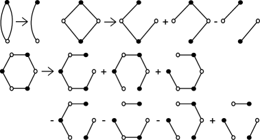
Figure 4. Local transformations on graphs.

Then we have the following result:

Theorem 8.1 (Féray [Fér09]).

The coefficient of $R_{2}^{s_{2}}R_{3}^{s_{3}}\ldots$ in $K_{k}$ is equal to $(-1)^{1+s_{2}+s_{3}+\ldots}$ times the total sum of coefficients of all forests in $S$ which consist of $s_{i}$ trees with one black and $i-1$ white vertices ($i$ runs over $\{2,3,\dots\}$).

We will reformulate this result in a form closer to Theorem 1.4. For this purpose, if $(\sigma_{1},\sigma_{2},q)$ is a triple verifying conditions (a)–(d) and $F$ is a subforest of $\mathcal{V}^{\sigma_{1},\sigma_{2}}$ with the same set of vertices, we will say that $F$ is a $q$-forest if the following two conditions are fulfilled:

• all cycles of $\sigma_{2}$ (black vertices) are in different connected components,

• each cycle $c$ of $\sigma_{2}$ is the neighbor of exactly $q(c)-1$ cycles of $\sigma_{1}$ (white vertices).

Theorem 8.2.

Let $k\geq 1$ and let $s_{2},s_{3},\dots$ be a sequence of non-negative integers with only finitely many non-zero elements. The coefficient of the monomial $R_{2}^{s_{2}}R_{3}^{s_{3}}\cdots$ in the Kerov polynomial $K_{k}$ is equal to the number of triples $(\sigma_{1},\sigma_{2},q)$ which fulfill conditions (a)–(d) of Theorem 1.4 and such that

1. when we apply the transformations from Figure 4 as prescribed in [Fér09, Section 3], in the resulting linear combination of forests there is (exactly one) $q$-forest.

It is easy to see that this theorem is a reformulation of Theorem 8.1. A priori, it might seem that in the theorem above we should count each triplet $(\sigma_{1},\sigma_{2},q)$ with multiplicity equal to the number of $q$-forests appearing in the result, but we will prove in Corollary 8.4 that it is always equal to $0$ or $1$.

Comparing Theorem 8.2 with Theorem 1.4 we may wonder if conditions (e) and (e⁵) are equivalent. We will prove their equivalence in the following section.

8.2. Equivalence of conditions (e) and (e⁵)

In Section 1.9 we introduced the notion of $q$-admissibility of a graph. Recall that if a graph $G$ is connected then it is $q$-admissible if and only if it satisfies condition (e³) which is a reformulation of (e). Notice also that if $G$ contains no loops then it is $q$-admissible if and only if it is a $q$-forest.

Lemma 8.3.

The sum of coefficients of $q$-admissible graphs $G$ multiplied by $(-1)^{\text{(number of connected components of $G$)}}$ in a formal linear combination of bipartite graphs with a given set of vertices and labeling $q:V_{\bullet}\rightarrow\{2,3,\dots\}$ does not change after performing any transformation of the form presented on Figure 4.

Proof.

Let us choose some oriented loop $L$ in graph $G$ and let us denote by $E$ the set of edges which can be erased in the corresponding local transformation from Figure 4; in other words $E$ consists of every second edge in the loop $L$.

Consider the convex polyhedron $P$ (without boundary) which is the set of all positive solutions $(x_{e})_{\text{$e$ is an edge of $G$}}$ to the system of equations from condition (e⁴).

If $f$ is a real function on the set of edges of $G$ and $v$ is a vertex of $G$ we define $\big{(}\Phi(f)\big{)}(v)$ to be the sum of values of $f$ on edges adjacent to $v$. If $P$ is non-empty then its dimension is equal to the dimension of $\ker\Phi$. It is a simple exercise to show that $\operatorname{Im}\Phi$ consists of all functions on vertices of $G$ with a property that for each connected component of $G$ the sum of values on black vertices is equal to the sum of values on white vertices hence

$$\operatorname{dim}\operatorname{Im}\Phi=(\text{number of vertices of $G$})-(\text{number of components of $G$}).$$

It follows from rank-nullity theorem that

(42) $$\operatorname{dim}P=\operatorname{dim}\ker\Phi=\\ (\text{number of edges of $G$})-(\text{number of vertices of $G$})+\\ (\text{number of connected components of $G$}).$$

For a positive solution $(x_{e})$ of our system of equations and a real number $t$ we define

$$y_{e}=\begin{cases}x_{e}&\text{if }e\notin L,\\ x_{e}+t&\text{if }e\in(L\setminus E),\\ x_{e}-t&\text{if }e\in E.\end{cases}$$

which is also a solution. Let $t$ be the minimal positive number for which $(y_{e})$ is not positive. In this way we define a map $\Pi:(x_{e})\mapsto(y_{e})$.

For any non-empty $A\subseteq E$ we define $P_{A}$ to be the set of positive solutions with a property that

$$\forall_{e\in E}\quad e\in A\iff x_{e}=\min_{f\in E}x_{f}.$$

Since the defining condition for $P_{A}$ can be written in terms of some equations and inequalities it follows that $P_{A}$ is a convex polyhedron. It is easy to check that

$$\Pi(P_{A})=\big{\{}(x_{e}):\text{non-negative solution such that }\\ \forall_{e:\text{ edge of G}}\quad(x_{e}=0)\iff(e\in A)\big{\}}.$$

The latter set can be identified with the set of positive solutions for our system of equations corresponding to the graph $G^{\prime}=G\setminus A$. It follows that

(43) $$\operatorname{dim}P_{A}=1+\operatorname{dim}\Pi(P_{A})=\\ 1+\left(\text{number of edges of $(G\setminus A)$}\right)-(\text{number of vertices of $G$})+\\ \left(\text{number of connected components of $(G\setminus A)$}\right),$$

where the last equality is just (42) applied to $G^{\prime}=G\setminus A$.

It is easy to see that $P=\bigsqcup_{A\neq\emptyset}P_{A}$ is a disjoint union therefore we have the equality between the Euler characteristics:

$$\chi(P)=\sum_{A\neq\emptyset}\chi(P_{A})$$

which thanks to (42) and (43) shows that

(44) $$(-1)^{(\text{number of connected components of $G$})}\ [\text{$P$ is non-empty}]=\\ \sum_{A\neq\emptyset}(-1)^{|A|-1}\ (-1)^{(\text{number of components of $G\setminus A$})}\ [\text{$P_{A}$ is non-empty}],$$

where we use the convention that

$$[\text{(condition)}]=\begin{cases}1&\text{if (condition) is true},\\ 0&\text{otherwise}.\end{cases}$$

Proposition 1.9 shows that $P$ (respectively, $P_{A}$) is non-empty if and only if $G$ (respectively, $G\setminus A$) is $q$-admissible therefore (44) is equivalent to

$$(-1)^{(\text{number of components of $G$})}\ [\text{$G$ is $q$-admissible}]=\\ \sum_{A\neq\emptyset}(-1)^{|A|-1}\ (-1)^{(\text{number of components of $G\setminus A$})}\ [\text{$(G\setminus A)$ is $q$-admissible}],$$

which is the desired equality. ∎

Corollary 8.4.

Suppose that $(\sigma_{1},\sigma_{2},q)$ is a triple verifying the conditions (a)–(d) of Theorem 1.4. If we iterate local transformations from Figure 4 on $\mathcal{V}^{\sigma_{1},\sigma_{2}}$ until we obtain a formal linear combination of forests (not necessarily choosing the loops as prescribed in [Fér09]) then the sum of coefficients of $q$-forests in the result is equal to

$$\begin{cases}(-1)^{1+s_{2}+s_{3}+\ldots}&\text{if condition \ref{enum:marriage} is fulfilled;}\\ 0&\text{otherwise.}\end{cases}$$

In the case when we perform the transformations as prescribed in [Fér09, Section 3], the sign property of this decomposition ([Fér09, Proposition 3.3.1]) implies that there is exactly one $q$-forest (with the appropriate sign) in the resulting sum if condition (e) is fulfilled and there are no $q$-forests otherwise; in other words condition (e) is equivalent to (e⁵).

The above corollary together with Theorem 8.2 give another proof of the main result of the paper, Theorem 1.4. Analogous results can be stated for the situation presented in Theorem 1.6.

Appendix A Results obtained after this paper has been submitted for publication

In this appendix we present results which became available after this paper has been submitted for publication. Thus they are not contained in the version published in Advances in Mathematics.

A.1. Closed walk interpretation of condition (e)

Proposition A.1.

Condition (e) is equivalent to the following one:

1. it is possible to chose orientations on the edges of the bipartite graph $\mathcal{V}^{\sigma_{1},\sigma_{2}}$ in such a way that:

   • every white vertex has exactly one outgoing edge and every black vertex $j\in C(\sigma_{2})$ has exactly $q(j)-1$ incoming edges,

   • if we interpret orientations of edges as directions of one-way streets, there exists a closed walk in the graph such that every black vertex is visited at least once.

Proof.

There is a bijective correspondence between the arrangements of marriages as in Section 1.8 and the arrangements of orientations of edges given as follows: for any pair $i\in C(\sigma_{1})$, $j\in C(\sigma_{2})$ of connected vertices, if a boy $i$ is married to a girl $j$, we draw an oriented edge from vertex $i$ to vertex $j$; otherwise we draw an oriented edge in the opposite direction.

Assume that condition (e) holds true. Condition (e²) shows that it is possible to arrange marriages; we fix the corresponding orientations of the edges. Let $j\in C(\sigma_{2})$ be a black vertex and let $A\subseteq C(\sigma_{2})$ (respectively, $B\subseteq C(\sigma_{1})$) be the set of black (respectively, white) vertices $j^{\prime}$ with a property that there exists a walk from $j^{\prime}$ to $j$. It is easy to see that the set of husbands of $A$ is equal to $B$. Furthermore, every vertex in $B$ is connected only to vertices from $A$, therefore it is not possible arrange marriages so that the set of wives of $B$ is different from $A$; therefore it is not possible to arrange marriages so that the set of husbands of $A$ is different from $B$. From condition (e²) it follows that $A=C(\sigma_{2})$. In this way we proved that any two black vertices can be connected by a walk. By combining such walks we get the desired closed walk which visits every black vertex at least once.

Conversely, assume that condition (e^enumi) holds true and let $A\varsubsetneq C(\sigma_{2})$, $A\neq\emptyset$ be a non-trivial subset. The choice of orientations of the edges in the graph gives rise to some choice of marriages. We denote by $B\subseteq C(\sigma_{1})$ the set of husbands of $A$. In the closed walk $(\dots,j,i,\dots)$ given by condition (e^enumi) there must be a neighboring pair of vertices such that $j\in A\cup B$ and $i\notin A\cup B$. It is easy to see that it is only possible if $j\in A$ and $i\in C(\sigma_{1})\setminus B$. This shows that the set of possible husbands for $A$ contains $B\sqcup\{i\}$ as a subset therefore condition (e) is fulfilled. ∎

A.2. General formula for Kerov polynomials

Theorem A.2.

Let $\mathcal{G}$ be a finite collection of connected bipartite graphs and let $\mathcal{G}\ni G\mapsto m_{G}$ be a scalar-valued function on it. We assume that

$$F(\lambda)=\sum_{G\in\mathcal{G}}m_{G}\ N_{G}(\lambda)$$

is a polynomial function on the set of Young diagrams; in other words $F$ can be expressed as a polynomial in free cumulants.

Let $s_{2},s_{3},\dots$ be a sequence of non-negative integers with only finitely many non-zero elements; then

$$\left[R_{2}^{s_{2}}R_{3}^{s_{3}}\cdots\right]F=(-1)^{s_{2}+2s_{3}+3s_{4}+\cdots+1}\sum_{G\in\mathcal{G}}\sum_{q}m_{G},$$

where the sums runs over $G\in\mathcal{G}$ and $q$ such that:

1. the number of the black vertices of $G$ is equal to $s_{2}+s_{3}+\cdots$;

2. the total number of vertices of $G$ is equal to $2s_{2}+3s_{3}+4s_{4}+\cdots$;

3. $q$ is a function from the set of the black vertices to the set $\{2,3,\dots\}$; we require that each number $i\in\{2,3,\dots\}$ is used exactly $s_{i}$ times;

4. for every subset $A\subset V_{\circ}(G)$ of black vertices of $G$ which is nontrivial (i.e., $A\neq\emptyset$ and $A\neq V_{\circ}(G)$) there are more than $\sum_{v\in A}\big{(}q(v)-1\big{)}$ white vertices which are connected to at least one vertex from $A$.

In this paper we proved this result in the special case when $F=\Sigma_{n}$ and $\mathcal{G}$ is the (signed) collection of bipartite maps corresponding to all factorizations of a cycle, however it is not difficult to verify that the proof presented in this article works without any modifications also in this more general setup.

References

- [Bia07] Philippe Biane. On the formula of Goulden and Rattan for Kerov polynomials. Sém. Lothar. Combin., 55:Art. B55d, 5 pp. (electronic), 2005/07.
- [Bia98] Philippe Biane. Representations of symmetric groups and free probability. Adv. Math., 138(1):126–181, 1998.
- [Bia01] Philippe Biane. Free cumulants and representations of large symmetric groups. In XIIIth International Congress on Mathematical Physics (London, 2000), pages 321–326. Int. Press, Boston, MA, 2001.
- [Bia03] Philippe Biane. Characters of symmetric groups and free cumulants. In Asymptotic combinatorics with applications to mathematical physics (St. Petersburg, 2001), volume 1815 of Lecture Notes in Math., pages 185–200. Springer, Berlin, 2003.
- [CGS04] Sylvie Corteel, Alain Goupil, and Gilles Schaeffer. Content evaluation and class symmetric functions. Adv. Math., 188(2):315–336, 2004.
- [Fér06] Valentin Féray. Proof of Stanley’s conjecture about irreducible character values of the symmetric group. Preprint arXiv:math.CO/0612090, 2006.
- [Fér09] Valentin Féray. Combinatorial interpretation and positivity of Kerov’s character polynomials. J. Algebraic Combin., 29(4):473–507, 2009.
- [FŚ07] Valentin Féray and Piotr Śniady. Asymptotics of characters of symmetric groups related to Stanley-Féray character formula. Preprint arXiv:math/0701051, 2007.
- [GR07] I. P. Goulden and A. Rattan. An explicit form for Kerov’s character polynomials. Trans. Amer. Math. Soc., 359(8):3669–3685 (electronic), 2007.
- [IO02] Vladimir Ivanov and Grigori Olshanski. Kerov’s central limit theorem for the Plancherel measure on Young diagrams. In Symmetric functions 2001: surveys of developments and perspectives, volume 74 of NATO Sci. Ser. II Math. Phys. Chem., pages 93–151. Kluwer Acad. Publ., Dordrecht, 2002.
- [Ker98] Sergei Kerov. Interlacing measures. In Kirillov’s seminar on representation theory, volume 181 of Amer. Math. Soc. Transl. Ser. 2, pages 35–83. Amer. Math. Soc., Providence, RI, 1998.
- [Ker99] S. Kerov. A differential model for the growth of Young diagrams. In Proceedings of the St. Petersburg Mathematical Society, Vol. IV, volume 188 of Amer. Math. Soc. Transl. Ser. 2, pages 111–130, Providence, RI, 1999. Amer. Math. Soc.
- [Ker00] S. Kerov. Talk in Institute Henri Poincaré, Paris, January 2000.
- [Ker03] S. V. Kerov. Asymptotic representation theory of the symmetric group and its applications in analysis, volume 219 of Translations of Mathematical Monographs. American Mathematical Society, Providence, RI, 2003. Translated from the Russian manuscript by N. V. Tsilevich, With a foreword by A. Vershik and comments by G. Olshanski.
- [Las08] Michel Lassalle. Two positivty conjectures for Kerov polynomials. Adv. in Appl. Math., 41(3):407–422, 2008.
- [LS77] B. F. Logan and L. A. Shepp. A variational problem for random Young tableaux. Advances in Math., 26(2):206–222, 1977.
- [LZ04] Sergei K. Lando and Alexander K. Zvonkin. Graphs on surfaces and their applications, volume 141 of Encyclopaedia of Mathematical Sciences. Springer-Verlag, Berlin, 2004. With an appendix by Don B. Zagier, Low-Dimensional Topology, II.
- [Roi96] Yuval Roichman. Upper bound on the characters of the symmetric groups. Invent. Math., 125(3):451–485, 1996.
- [RŚ08] Amarpreet Rattan and Piotr Śniady. Upper bound on the characters of the symmetric groups for balanced Young diagrams and a generalized Frobenius formula. Adv. Math., 218(3):673–695, 2008.
- [Śni06a] Piotr Śniady. Asymptotics of characters of symmetric groups, genus expansion and free probability. Discrete Math., 306(7):624–665, 2006.
- [Śni06b] Piotr Śniady. Gaussian fluctuations of characters of symmetric groups and of Young diagrams. Probab. Theory Related Fields, 136(2):263–297, 2006.
- [Spe93] Roland Speicher. The lattice of admissible partitions. In Quantum probability & related topics, QP-PQ, VIII, pages 347–352. World Sci. Publ., River Edge, NJ, 1993.
- [Spe98] Roland Speicher. Combinatorial theory of the free product with amalgamation and operator-valued free probability theory. Mem. Amer. Math. Soc., 132(627):x+88, 1998.
- [Sta04] Richard P. Stanley. Irreducible symmetric group characters of rectangular shape. Sém. Lothar. Combin., 50:Art. B50d, 11 pp. (electronic), 2003/04.
- [Sta02] Richard P. Stanley. Kerov’s character polynomial and irreducible symmetric group characters of rectangular shape. Transparencies from a conference in Québec City, June 2002.
- [Sta06] Richard P. Stanley. A conjectured combinatorial interpretation of the normalized irreducible character values of the symmetric group. Preprint arXiv:math.CO/0606467, 2006.
- [VDN92] D. V. Voiculescu, K. J. Dykema, and A. Nica. Free random variables, volume 1 of CRM Monograph Series. American Mathematical Society, Providence, RI, 1992. A noncommutative probability approach to free products with applications to random matrices, operator algebras and harmonic analysis on free groups.
- [VK77] A. M. Veršik and S. V. Kerov. Asymptotic behavior of the Plancherel measure of the symmetric group and the limit form of Young tableaux. Dokl. Akad. Nauk SSSR, 233(6):1024–1027, 1977.
- [Voi86] Dan Voiculescu. Addition of certain noncommuting random variables. J. Funct. Anal., 66(3):323–346, 1986.
- [Voi91] Dan Voiculescu. Limit laws for random matrices and free products. Invent. Math., 104(1):201–220, 1991.