Distributed Estimation over Wireless Sensor Networks
with Packet Losses

Abstract

A distributed adaptive algorithm to estimate a time-varying signal, measured by a wireless sensor network, is designed and analyzed. One of the major features of the algorithm is that no central coordination among the nodes needs to be assumed. The measurements taken by the nodes of the network are affected by noise, and the communication among the nodes is subject to packet losses. Nodes exchange local estimates and measurements with neighboring nodes. Each node of the network locally computes adaptive weights that minimize the estimation error variance. Decentralized conditions on the weights, needed for the convergence of the estimation error throughout the overall network, are presented. A Lipschitz optimization problem is posed to guarantee stability and the minimization of the variance. An efficient strategy to distribute the computation of the optimal solution is investigated. A theoretical performance analysis of the distributed algorithm is carried out both in the presence of perfect and lossy links. Numerical simulations illustrate performance for various network topologies and packet loss probabilities.

Keywords: Distributed Estimation; Wireless Sensor Networks; Parallel and Distributed Computation; Convex Optimization; Lipschitz Optimization.

1 Introduction

Monitoring physical variables is a typical task performed by wireless sensor networks (WSNs). Accurate estimation of these variables is a major need for many applications, spanning from traffic control, industrial manufacturing automation, environment monitoring, to security systems [1]–[3]. However, nodes of WSNs have limitations, such as scarcity of energy supply, lightweight processing and communication functionalities, with the consequence that sensed data are affected by bias and noise, and transmission is subject to interference, which results in corrupted data (packet loss). Estimation algorithms must be designed to cope with these adverse conditions, while offering high accuracy.

There are two main estimation strategies for WSNs. A traditional approach consists in letting nodes sense the environment and then report data to a central unit, which extracts the desired physical variable and sends the estimate to each local node for local action. However, this approach has strong limitations: large amount of communication resources (radio power, bandwidth, routing, etc.) have to be managed for the transmission of information from nodes to the central unit and vice versa, which reduces the nodes’ lifetime. An alternative approach, which we investigate in this paper, enables each node to locally produce accurate estimates taking advantage of data exchanged with only neighboring nodes. Indeed, wireless communication makes it natural to exploit cooperative strategies, as it has been already used for coding and transmission [3, 4]. The challenge of distributed estimation is that local processing must be carefully designed to avoid heavy computations and spreading of local errors throughout the network.

In this paper we consider the design and analysis of a distributed estimation algorithm. Specifically, a time-varying signal is jointly tracked by the nodes of a WSN, in which each node computes an estimate as a weighted sum of its own and its neighbors’ measurements and estimates. The distributed estimator features three particular characteristics: it is robust to packet losses, it does not rely on a model of the signal to track, and it uses filter coefficients that adapt to the changing network topology caused by packet losses. We show that the estimation problem has a distributed implementation. It is argued that the estimator exhibits high accuracy, in term of estimation error variance, even in the presence of severe packet losses, if the signal to track is varying slowly.

1.1 Related Work

The estimator presented in this paper is related to recent contributions on low-pass filtering by diffusion mechanisms, e.g., [5]–[12], where each node of the network obtains the average of the initial samples collected by nodes. In [13, 14] the authors study a distributed average computation of a time-varying signal, when the signal is affected by a zero-mean noise. Distributed filtering using model-based approaches is studied in various wireless network contexts, e.g., [11], [15]–[18]. In particular, distributed Kalman filters and more recently a combination of the diffusion mechanism with distributed Kalman filtering have been proposed, e.g., [19].

In [20], we have presented a distributed estimator to track a time-varying signal without relaying on a model of the signal to track, in contrast to model-based approaches, e.g., [11, 16]. The approach is novel, since [8]–[10] are limited to averaging initial samples. Compared to [10]–[14] and [17]–[19], we do not rely on the Laplacian matrix associated to the communication graph. Our filter parameters are computed through distributed algorithms which adapt to the network topology and packet losses, whereas for example [13] and [14] rely on centralized algorithms for designing the filters. The distributed estimator proposed in this paper features better estimates when compared to similar distributed algorithms presented in the literature, but at the cost of a slightly increased computational complexity. With respect to our earlier work [20], here we provide a major extension because we take into account lossy wireless communications. Packet losses require a substantial redesign and performance characterization of the filter proposed in [20]. In this paper, we explicitly consider the effect of packet losses (both i.i.d. and non-identical) in the design of the adaptive weights so that the estimation error is guaranteed to converge for any packet loss realization. The distributed minimum variance estimator uses a Lipschitz optimization problem to distribute the centralized stability constrains, whose characterization is completely new. We devise a new algorithm to distribute efficiently the computation of the solution of the Lipschitz problem. An original analysis of the bounds on the estimation error variance as function of the packet loss probability and number of nodes is also discussed. We introduce some examples to show how such bounds can be refined significantly when the network topology is modelled by a graph in the class of finite Cayley graphs.

The remainder of the paper is organized as follows: In Section 2 we review and extend the problem posed in [20] considering packet losses. In Section 3 we deal with the design of the optimal adaptive weights that minimize the estimation error variance. In Section 4 we show how to compute efficiently some thresholds needed to bound the norm of the estimation error. In Section 5 we determine bounds on the estimation error variance achieved by the proposed algorithm. Monte Carlo simulations are reported in Section 6 to illustrate the performance of the proposed algorithm. Conclusions are drawn in Section 7.

1.2 Notation

Given a stochastic variable $x$, $\,\mathds{E}\,x$ denotes its expected value. With $\,\mathds{E}\,_{y}x$ we mean that the expected value is taken with respect to the probability density function of $y$. We keep explicit the time dependence to remind the reader that the realization is given at time $t$. With $\|\cdot\|$ we denote the $\ell^{2}$-norm of a vector or the spectral norm of a matrix. Given a matrix ${\bf A}$, $\ell_{m}({\bf A})$ and $\ell_{M}({\bf A})$ denote the minimum and maximum eigenvalue (with respect to the absolute value of their real part), respectively, and its largest singular value is denoted by ${\gamma}({\bf A})$. Given the matrix ${\bf B}$, ${\bf A}\circ{\bf B}$ is the Hadamard (element-wise) product between ${\bf A}$ and ${\bf B}$. With ${\bf a}\preceq{\bf b}$ and ${\bf a}\succeq{\bf b}$ denote the element-wise inequalities. With ${\bf I}$ and $\mathbf{1}$ we denote the identity matrix and the vector $(1,\dots,1)^{T}$, respectively, whose dimensions are clear from the context. Let $\mathds{N}_{0}=\mathds{N}\cup\{0\}$. To keep the notation lighter, the time dependence of the variables and parameters is not explicitly indicated, when this does not create misunderstandings.

2 Problem Formulation

Consider a WSN with $N>1$ sensor nodes. At every time instant, each sensor in the network takes a noisy measure $u_{i}(t)$ of a scalar signal $d(t)$, namely $u_{i}(t)=d(t)+v_{i}(t)$, for $t\in\mathds{N}_{0}$ and for all $i=1,\dots,N$. We assume that $v_{i}(t)$, for all $i$, are normally distributed with zero mean and variance $\sigma^{2}$ and that $\,\mathds{E}\,v_{i}(t)v_{j}(t)=0$ for all $t\in\mathds{N}_{0}$.

We model the network as a weighted graph. In particular we consider a graph, $\mathcal{G}(t)=(\mathcal{V},\mathcal{E})$, where $\mathcal{V}=\{1,\dots,N\}$ is the vertex set and $\mathcal{E}\subseteq\mathcal{V}\times\mathcal{V}$ is the edge set.

The set of neighbors of node $i\in\mathcal{V}$ plus node $i$ is denoted as

$$\mathcal{N}_{i}=\{j\in\mathcal{V}:(j,i)\in\mathcal{E}\}\cup\{i\}\,,$$

Namely $\mathcal{N}_{i}$ is the set containing the maximum number of neighbors a node $i$ can have, including itself.

Every node broadcasts data packets, so that these packets can be received by any other node in the communication range. Packets may be dropped because of bad channel conditions or radio interference. Let $\phi_{ij}(t)$, with $i\neq j$, be a binary random variable associated to the packet losses from node $i$ to $j$ at time $t$ [21]. This random variable is defined on the probability space $(\Omega,\mathcal{F},\Pr)$, where $\Omega=\{0,1\}$, $\mathcal{F}$ is a $\sigma$-algebra of subsets of $\Omega$ and $\Pr(.)$ a probability measure. For $i\neq j$, we assume that the random variables $\phi_{ij}(t)$ are independent with probability mass function:

$$\Pr(\phi_{ij}(t)=1) =p_{ij}\,,$$

$$\Pr(\phi_{ij}(t)=0) =q_{ij}=1-p_{ij}\,,$$

where $p_{ij}\in[0,1]$ denotes the successful packet reception probability. Clearly that $p_{ii}=1$, since information locally available is not subject to packet losses. Note also that $p_{ji}=0$ if the packet sent from node $j$ to $i$ collided at node $i$ due to too much wireless interferences, or if the wireless channel of the link from $j$ to $i$ is under deep fading, or if $i$ is too far from node $j$ to receive packets from node $j$. The packet reception probabilities are assumed to be independent among links, and independent from past packet losses. These assumptions are natural when the coherence time of the wireless channel is small if compared to the typical communication rate of data packets over WSNs [21, 22].

We assume each node $i$ computes an estimate $x_{i}(t)$ of $d(t)$ by taking a linear combination of its own and of its neighbors’ estimates and measurements. Define $\mathbf{x}_{i}(t)=(x_{1}(t),\dots,x_{N}(t))^{T}$ and similarly $\mathbf{u}_{i}(t)=(u_{1}(t),\dots,u_{N}(t))^{T}$, then each node computes

$$x_{i}(t)=({\bf k}_{i}\boldsymbol{\phi}_{i})^{T}(t)\>\mathbf{x}_{i}(t-1)+({\bf h}_{i}\boldsymbol{\phi}_{i})^{T}(t)\>\mathbf{u}_{i}(t)\,,$$ (2.1)

with ${\bf x}_{i}(0)={\bf u}_{i}(0)$, and where

$$({\bf k}_{i}\boldsymbol{\phi}_{i})(t)={\bf k}_{i}^{T}(t)\circ\boldsymbol{\phi}_{i}^{T}(t)=\left(k_{1}(t),k_{2}(t),\dots,k_{N}(t)\right)^{T}\circ\left(\phi_{1}(t),\phi_{2}(t),\dots,\phi_{N}(t)\right)^{T}\,.$$

with ${\bf k}_{i}^{T}(t)\in\mathds{R}^{N}\times 1$, in which the $j$-th element is the weight coefficient used by node $i$ for information coming from node $j$ at time $t$, and $\boldsymbol{\phi}_{i}(t)\in\mathds{R}^{N}\times 1$ denotes the vector of the packet reception process as seen from node $i$ with respect to all nodes of the network. Specifically, the $j$th element of $\boldsymbol{\phi}_{i}(t)$, with $j\neq i$, be $\phi_{ij}(t)$. Let $\boldsymbol{\varphi}_{i|t}\in\Omega^{N}$ denotes a realization of the process $\boldsymbol{\phi}_{i}(t)$ at time $t$. Notice that at a given time instant, the $j$-th component of $\boldsymbol{\varphi}_{i|t}$ is zero if no data packets are received from node $j$. Let $\mathcal{N}_{\boldsymbol{\varphi}_{i}}=\{j\in\mathcal{N}_{i}:\boldsymbol{\varphi}_{i_{j}|t}\neq 0\}$, namely a such set collects the nodes communicating with node $i$ at time $t$. The number of nodes in the set is $|\mathcal{N}_{\boldsymbol{\varphi}_{i}}|=\boldsymbol{\varphi}_{i|t}^{T}\boldsymbol{\varphi}_{i|t}$.

The vector $({\bf h}_{i}\boldsymbol{\phi}_{i})(t)\in\mathds{R}^{N\times 1}$ and ${\bf h}_{i}^{T}(t)\in\mathds{R}^{N\times 1}$ are constructed from the elements $h_{ij}(t)$, similarly to $({\bf k}_{i}\boldsymbol{\phi}_{i})(t)$.

3 Distributed Minimum Variance Estimator

In this section we describe how each node computes adaptive weights to minimize its estimation error variance.

3.1 Estimation Error

Define the estimation error at node $i$ as $e_{i}(t)=x_{i}(t)-d(t)\mathbf{1}$. Introduce $\delta(t)=d(t)-d(t-1)$, then the expected error with respect to the measurement noise $\mathbf{v}_{i}(t)=(v_{1}(t),\dots,v_{N}(t))^{T}$ is given by

$$\,\mathds{E}\,_{\bf v}e_{i}(t)=({\bf k}_{i}\boldsymbol{\phi}_{i})^{T}(t)\>\,\mathds{E}\,_{v}\mathbf{e}_{i}(t-1)+d(t)\left(({\bf k}_{i}\boldsymbol{\phi}_{i})^{T}(t)\>\mathbf{1}+({\bf h}_{i}\boldsymbol{\phi}_{i})^{T}(t)\>\mathbf{1}-1\right)-\delta(t)({\bf k}_{i}\boldsymbol{\phi}_{i})^{T}(t)\mathbf{1}\,,$$ (3.1)

where we set $\mathbf{e}_{i}(t)=(e_{1}(t),\dots,e_{N}(t))^{T}$.

Typically one is interested in designing an unbiased estimator. Notice, however that in (3.1) the expected error depends on both unknowns $d(t)$ and $\delta(t)$. The following condition eliminates the dependence from $d(t)$:

$$({\bf k}_{i}\boldsymbol{\phi}_{i})^{T}(t)\>\mathbf{1}+({\bf h}_{i}\boldsymbol{\phi}_{i})^{T}(t)\>\mathbf{1}=1\,,$$ (3.2)

for any possible realization of the packet loss process $\boldsymbol{\phi}_{i}(t)$. Note that (3.2) holds both in the presence of packet i.i.d. losses , and in the presence of non-identical losses. The term $\delta(t)$ can be removed by imposing that

$$({\bf k}_{i}\boldsymbol{\phi}_{i})^{T}(t)\>\mathbf{1}=0\,,$$ (3.3)

for any possible realization of the packet loss process $\boldsymbol{\phi}_{i}(t)$. By imposing constraints (3.2) and (3.3), the unknown terms would disappear from the expected error equation, so the minimum variance estimator would be such that $({\bf k}_{i}\boldsymbol{\phi}_{i})^{T}(t)=\mathbf{0}$ and $({\bf h}_{i}\boldsymbol{\phi}_{i})^{T}(t)=1/|\mathcal{N}_{\boldsymbol{\varphi}_{i}}|\mathbf{1}$, where $|\mathcal{N}_{\boldsymbol{\varphi}_{i}}|$ is the number of neighbors, including node $i$, that are successfully communicating with node $i$ at time $t$. We will show in the next sections that by imposing only constraint (3.2) we are able to design an estimator that has lower variance than one that also obey (3.3). The price paid for better performance is a biased estimator. However, assuming that $d(t)$ is slowly varying (or that the sampling frequency is high enough with resect to the variation of the signal), the bias is negligible and the proposed estimator outperforms the unbiased one in terms of the estimation error variance. This can also be understood from an intuitive point of view: having $({\bf k}_{i}\boldsymbol{\phi}_{i})^{T}(t)=\mathbf{0}$ means that nodes are disregarding previous estimates and are just using current measurements, which are typically corrupted by high noise. Having a term that also weights previous estimates allows us to increment the total available information at each node, obtaining a much lower estimation error variance.

Notice that although (3.2) holds, and thus $d(t)$ is eliminated from (3.1), we need further conditions on vector $({\bf k}_{i}\boldsymbol{\phi}_{i})(t)$ in order to guarantee that the expected error asymptotically decreases.

3.2 Convergence of Estimation Error

In this subsection we derive conditions on the weights that ensure that the estimation error decreasing over time, regardless the measurement noise and the packet loss processes that affect the system. In particular, we want to determine conditions on the weights so that $|\,\mathds{E}\,_{\boldsymbol{\phi}}\,\mathds{E}\,_{\bf v}e_{i}(t)|\rightarrow 0$ as $t\rightarrow+\infty$.

Assume that constraint (3.2) holds, and consider the expected value with respect to the packet loss process of (3.1), then

$$\,\mathds{E}\,_{\boldsymbol{\phi}}\,\mathds{E}\,_{\bf v}e_{i}(t)=\,\mathds{E}\,_{\boldsymbol{\phi}}({\bf k}_{i}^{T}(t)\circ\boldsymbol{\phi}_{i}(t)^{T})\,\mathds{E}\,_{\boldsymbol{\phi}}\,\mathds{E}\,_{\bf v}\mathbf{e}_{i}(t-1)-\delta(t)\,\mathds{E}\,_{\boldsymbol{\phi}}({\bf h}_{i}^{T}(t)\circ\boldsymbol{\phi}_{i}(t)^{T})\>\mathbf{1}\,,$$

where we have used the fact that the packet losses at time $t$ are independent from the preceding time instants, so that $\,\mathds{E}\,_{\boldsymbol{\phi}}({\bf k}_{i}^{T}(t)\circ\boldsymbol{\phi}_{i}(t)^{T}\,\mathds{E}\,_{\bf v}\mathbf{e}_{i}(t-1))=\,\mathds{E}\,_{\boldsymbol{\phi}}({\bf k}_{i}^{T}(t)\circ\boldsymbol{\phi}_{i}(t)^{T})\,\mathds{E}\,_{\boldsymbol{\phi}}\,\mathds{E}\,_{\bf v}\mathbf{e}_{i}(t-1)$. It is clear that the evolution of $\,\mathds{E}\,_{\boldsymbol{\phi}}\,\mathds{E}\,_{\bf v}e_{i}(t)$ depends on the overall error vector $\mathbf{e}_{i}(t-1)$, namely, the error at the local node depends on the estimation error of neighboring nodes. We thus need a set of other $|\mathcal{N}_{i}|-1$ equations to describe the estimation error of all nodes in $\mathcal{N}_{i}$. Obviously, each new equation will depend on the estimation error of nodes that are two hops from node $i$, and so on. The full network will be considered in this process of adding equations. Let $\mathbf{e}(t)\in\mathds{R}^{N}$ be the estimation error of the overall network, then

$$\,\mathds{E}\,_{\boldsymbol{\phi}}\,\mathds{E}\,_{\bf v}\mathbf{e}(t)=\,\mathds{E}\,_{\boldsymbol{\phi}}({\bf K}(t)\circ\Phi(t))\,\mathds{E}\,_{\phi}\,\mathds{E}\,_{v}\mathbf{e}(t-1)-\delta(t)\,\mathds{E}\,_{\boldsymbol{\phi}}({\bf H}(t)\circ\Phi(t))\mathbf{1}\,,$$ (3.4)

where ${\bf K}(t)=\left({\bf k}_{1}(t),{\bf k}_{2}(t),\dots,{\bf k}_{N}(t)\right)^{T}$ is the matrix whose rows are the vectors ${\bf k}_{i}^{T}(t)$, $i=1,\dots,N$, and $\Phi(t)=\left(\boldsymbol{\phi}_{1}(t),\boldsymbol{\phi}_{2}(t),\dots,\boldsymbol{\phi}_{N}(t)\right)^{T}$ is the matrix whose rows are the vectors $\boldsymbol{\phi}_{i}^{T}(t)$, $i=1,\dots,N$. Let $\boldsymbol{\varphi}_{|t}$ be a realization of $\Phi(t)$ at time $t$, namely $\boldsymbol{\varphi}_{|t}=\left(\boldsymbol{\varphi}_{1|t},\boldsymbol{\varphi}_{2|t},\dots,\boldsymbol{\varphi}_{N|t}\right)^{T}$. The following result holds:

Proposition 3.1.

Consider the system (3.4) and assume that

• $\gamma({\bf K}(t)\circ\boldsymbol{\varphi}_{|t})\leq\gamma_{\max}<1$ for all $t\in\mathds{N}_{0}$ and for each and every packet loss realization $\boldsymbol{\varphi}_{|t}$ of $\Phi(t)$.

• $|\delta(t)|<\Delta$ for all $t\in\mathds{N}_{0}$.

Then, considering independent packet losses, we have that

$$\lim_{t\rightarrow+\infty}\|\,\mathds{E}\,_{\boldsymbol{\phi}}\,\mathds{E}\,_{\bf v}\mathbf{e}(t)\|\leq\frac{\Delta\sqrt{N}\gamma_{\max}}{1-\gamma_{\max}}\,.$$ (3.5)

Proof.

For the sake of notational simplicity, define $\mathbf{s}(t)=\,\mathds{E}\,_{\boldsymbol{\phi}}\,\mathds{E}\,_{\bf v}\mathbf{e}(t)$. The dynamics of $\mathbf{s}(t)$ are thus given by a deterministic time-varying linear system. Consider the function $V(\mathbf{s}(t))=\|\mathbf{s}(t)\|$. Simple algebra gives that

$$V(\mathbf{s}(t)) \leq\|\,\mathds{E}\,_{\boldsymbol{\phi}}({\bf K}(t)\circ\Phi(t))\|V(\mathbf{s}(t-1))+\|\,\mathds{E}\,_{\boldsymbol{\phi}}({\bf K}(t)\circ\Phi(t))\|\Delta\sqrt{N}\,.$$

Now, consider that

$$\,\mathds{E}\,_{\boldsymbol{\phi}}({\bf K}(t)\circ\Phi(t))=\sum_{\boldsymbol{\varphi}_{|t}\in\>\Sigma}({\bf K}(t)\circ\boldsymbol{\varphi}_{|t})\Pr(\boldsymbol{\varphi}_{|t})\,,$$

where $\Pr(\boldsymbol{\varphi}_{|t})$ is the probability of the packet reception realization $\boldsymbol{\varphi}_{|t}$ at time $t$. The expectation is given by the sum of a finite number of combinations $\Sigma$ of possible packet loss realizations, since the network has a finite number of links, and in each link a packet can be either successfully received or dropped, so that $|\Sigma|=2^{|\mathcal{E}|}$. It follows

$$\|\,\mathds{E}\,_{\boldsymbol{\phi}}{\bf K}(t)\circ\Phi(t)\|=\|\sum_{\boldsymbol{\varphi}_{|t}\in\>\Sigma}({\bf K}(t)\circ\boldsymbol{\varphi}_{|t})\Pr(\boldsymbol{\varphi}_{|t})\|\leq\sum_{\boldsymbol{\varphi}_{|t}\in\>\Sigma}\|{\bf K}(t)\circ\boldsymbol{\varphi}_{|t}\|\Pr(\boldsymbol{\varphi}_{|t})\leq\gamma_{\max}\,,$$

because obviously $\sum_{\boldsymbol{\varphi}_{|t}\in\>\Sigma}\Pr(\boldsymbol{\varphi}_{|t})=1$, and, from assumption (i), $\|{\bf K}(t)\circ\boldsymbol{\varphi}_{|t}\|\leq\gamma_{\max}<1$. Therefore

$$V(\mathbf{s}(t))\leq\gamma_{\max}^{t}V(\mathbf{s}(t-1))+\gamma_{\max}\frac{1-\gamma_{\max}^{t}}{1-\gamma_{\max}}\Delta\sqrt{N}\,,$$

from where, taking the limit $t\rightarrow+\infty$, the proposition follows. ∎

Remark 3.2.

Notice that the expected error converges to a neighborhood of the origin exponentially fast, and more precisely with rate $\gamma_{\max}<1$.

Proposition 3.1 provides us with conditions for the convergence of the estimation error of the entire network to a neighborhood of the origin. It follows that the estimation error of the entire network is subject to a cumulative bias. It is clear that such a bias depends on $\|{\bf K}(t)\circ\boldsymbol{\varphi}_{|t}\|$ and $\Delta$. If the signal $d(t)$ is slowly varying, namely $\Delta\ll 1$, and $\|{\bf K}(t)\circ\boldsymbol{\varphi}_{|t}\|$ small, then the bias will be small.

Notice that, in order to ensure that the estimation error decreases at each node, a condition at network level is required, namely it must hold that $\gamma({\bf K}(t)\circ\boldsymbol{\varphi}_{|t})\leq\gamma_{\max}<1$. The constant $\gamma_{\max}$ can be chosen by fixing a maximum cumulative estimation error and solving (3.5) for $\gamma_{\max}$, as we show in Section 6.

We will show in the next subsection how to choose the weights ${\bf k}_{i}(t)$ and ${\bf h}_{i}(t)$ locally at each node so that the estimation error variance is minimized.

3.3 Distributed Computation of Filter Coefficients

To design a minimum variance distributed estimator, we need to consider how the error variance evolves over time. The estimation error variance dynamic at node $i$ is given by

$$\,\mathds{E}\,_{\bf v}(e_{i}(t)-\,\mathds{E}\,_{\bf v}e_{i}(t))^{2}=({\bf k}_{i}\boldsymbol{\phi}_{i})^{T}(t){\bf P}_{i}(t-1)({\bf k}_{i}\boldsymbol{\phi}_{i})(t)+\sigma^{2}({\bf h}_{i}\boldsymbol{\phi}_{i})^{T}(t)({\bf h}_{i}\boldsymbol{\phi}_{i})(t)$$ (3.6)

where

$${\bf P}_{i}(t-1)=\,\mathds{E}\,(\mathbf{e}_{i}(t)-\,\mathds{E}\,\mathbf{e}_{i}(t))\,\mathds{E}\,(\mathbf{e}_{i}(t)-\,\mathds{E}\,\mathbf{e}_{i}(t))^{T}\in\mathds{R}^{N\times N}\,.$$

We assume that ${\bf x}_{i}(0)={\bf u}_{i}(0)$, and

$${\bf e}_{i}(0)={\bf u}_{i}(0)-\frac{1}{|\mathcal{N}_{\boldsymbol{\varphi}_{i}}|-1}\mathop{\sum_{j=1}^{|\mathcal{N}_{\boldsymbol{\varphi}_{i}}|}}_{j\neq i}{\bf u}_{j}(0)\,,$$

because an initial (rough) estimate of $d(0)$ can be computed as arithmetic average of the $|\mathcal{N}_{\boldsymbol{\varphi}_{i}}|-1$ measurements received from neighboring nodes.

The estimation error variance (3.6) can be rewritten as

$$\,\mathds{E}\,_{\bf v}(e_{i}(t)-\,\mathds{E}\,_{\bf v}e_{i}(t))^{2}={\bf k}_{i}^{T}(t)\left({\bf P}_{i}(t-1)\circ(\boldsymbol{\phi}_{i}(t)\boldsymbol{\phi}_{i}^{T}(t))\right){\bf k}_{i}(t)+\sigma^{2}{\bf h}_{i}^{T}(t)\boldsymbol{\phi}_{i}(t)\boldsymbol{\phi}_{i}^{T}(t){\bf h}_{i}^{T}(t)$$

where we used the fact that $\mathbf{a}^{T}\mathbf{B}\mathbf{a}={\rm tr}\,(\mathbf{B}\mathbf{aa}^{T})$ and ${\rm tr}\,(\mathbf{A}\circ\mathbf{B})\mathbf{C}={\rm tr}\,(\mathbf{C}^{T}\circ\mathbf{B})\mathbf{A}^{T}$.

The optimal weights ${\bf k}_{i}(t)$ and ${\bf h}_{i}(t)$ are chosen so that at each time instant, for any given realization of the packet loss process $\boldsymbol{\varphi}_{i}{|t}$ of $\boldsymbol{\phi}_{i}(t)$, the variance $E_{\bf v}(e_{i}(t)-\,\mathds{E}\,_{\bf v}e_{i}(t)|\boldsymbol{\phi}_{i}(t)=\boldsymbol{\varphi}_{i|t})^{2}$ is minimized, under the constrain (3.2) and that $\gamma({\bf K}(t)\circ\boldsymbol{\varphi}_{|t})\leq\gamma_{\max}<1$. As already mentioned, the second constraint is global, since ${\bf K}(t)\circ\boldsymbol{\varphi}_{|t}$ depends on all ${\bf k}_{i}(t)$, $i=1,\ldots,N$. However, it is possible to determine local conditions so that the global constraint is satisfied. We show next how this can be done.

For $i=1,\dots,N$, we define the set $\Theta_{\boldsymbol{\varphi}_{i}}=\{j\neq i:\mathcal{N}_{\boldsymbol{\varphi}_{i}}\cap\mathcal{N}_{\boldsymbol{\varphi}_{j}}\neq\emptyset\}\cup\{\mathcal{N}_{\boldsymbol{\varphi}_{i}}\}$, which is the collection of communicating nodes located at two hops distance from node $i$ plus communicating neighbors of $i$, at time $t$. The following result holds:

Proposition 3.3.

Suppose there exists $\boldsymbol{\psi}(t)=(\psi_{1}(t),\psi_{2}(t),\ldots,\psi_{N}(t))^{T}\succ 0$, such that

$$\psi_{i}(t)+\sqrt{\psi_{i}(t)}\sum_{j\in\Theta_{\boldsymbol{\varphi}_{i}}}\sqrt{\psi_{j}(t)}\leq\gamma_{\max}\quad\forall i\,.$$ (3.7)

If $\|{\bf k}_{i}(t)\circ\boldsymbol{\varphi}_{i|t}\|^{2}\leq\psi_{i}(t)$, $i=1,\dots,N$, then ${\gamma}({\bf K}(t)\circ\boldsymbol{\varphi}_{|t})\leq\gamma_{\max}<1$.

Proof.

The proof is similar to the proof of Proposition III.1 in [20]. ∎

Using this proposition, the global constraint ${\gamma}({\bf K}(t)\circ\boldsymbol{\varphi}_{|t})\leq\gamma_{\max}<1$ can be replaced by the constraint $\|{\bf k}_{i}(t)\circ\boldsymbol{\varphi}_{i|t}\|^{2}\leq\psi_{i}(t)$, where $\psi_{i}(t)$ satisfies the set of nonlinear inequalities (3.7). Therefore, each node needs to solve the following optimization problem

$$\min_{{\bf k}_{i}(t),{\bf h}_{i}(t)}\quad {\bf k}_{i}^{T}(t)\left({\bf P}_{i}(t-1)\circ(\boldsymbol{\varphi}_{i|t}\boldsymbol{\varphi}_{i|t}^{T})\right){\bf k}_{i}(t)+\sigma^{2}{\bf h}_{i}^{T}(t)\boldsymbol{\varphi}_{i|t}\boldsymbol{\varphi}_{i|t}^{T}{\bf h}_{i}(t)$$ (3.8)

s.t. $$\left(({\bf k}_{i}(t)+{\bf h}_{i}(t))^{T}\circ\boldsymbol{\varphi}_{i|t}\right)\mathbf{1}=1$$

$$\|{\bf k}_{i}(t)\circ\boldsymbol{\varphi}_{i|t}\|^{2}\leq\psi_{i}(t)\,.$$

We will discuss in Section 4 how to compute the values of $\psi_{i}(t)$, which are needed to state problem (3.8). Observe that the optimization problem (3.8) is a Quadratically Constrained Quadratic Problem [23, pag. 653]. It admits a strict interior point solution, corresponding to ${\bf k}_{i}(t)=0$ and $({\bf h}_{i}(t)\circ\boldsymbol{\varphi}_{i|t})\>\mathbf{1}=1$. Thus Slater’s condition is satisfied and strong duality holds [23, pag. 226]. The problem, however, does not have a closed form solution and thus we need to rely on numerical algorithms to derive the optimal ${\bf k}_{i}(t)$ and ${\bf h}_{i}(t)$. We have the following proposition.

Proposition 3.4.

For a given covariance matrix ${\bf P}_{i}(t-1)$ and a realization $\boldsymbol{\varphi}_{i|t}$ of $\boldsymbol{\phi}_{i}(t)$, the values of ${\bf k}_{i}(t)$ and ${\bf h}_{i}(t)$ that minimizes (3.8) are

$${\bf k}_{i}(t) =\frac{\left(({\bf P}_{i}(t-1)+\lambda_{i}(t){\bf I})\circ\boldsymbol{\varphi}_{i|t}\boldsymbol{\varphi}_{i|t}^{T}\right)^{\dagger}\boldsymbol{\varphi}_{i|t}}{\boldsymbol{\varphi}_{i|t}^{T}\left(\left(({\bf P}_{i}(t-1)+\lambda_{i}(t){\bf I})\circ\boldsymbol{\varphi}_{i|t}\boldsymbol{\varphi}_{i|t}^{T}\right)^{\dagger}+\sigma^{-2}{\bf I}\right)\boldsymbol{\varphi}_{i|t}}\,,$$ (3.9)

$${\bf h}_{i}(t) =\frac{\left(\boldsymbol{\varphi}_{i|t}\boldsymbol{\varphi}_{i|t}^{T}\right)^{\dagger}\boldsymbol{\varphi}_{i|t}}{\sigma^{2}\boldsymbol{\varphi}_{i|t}^{T}\left(\left(({\bf P}_{i}(t-1)+\lambda_{i}(t){\bf I})\circ\boldsymbol{\varphi}_{i|t}\boldsymbol{\varphi}_{i|t}^{T}\right)^{\dagger}+\sigma^{-2}{\bf I}\right)\boldsymbol{\varphi}_{i|t}}\,,$$ (3.10)

with the optimal Lagrange multiplier $\lambda_{i}(t)\in\left[0,\max\left(0,\sigma^{2}/\sqrt{|\mathcal{N}_{\boldsymbol{\varphi}_{i}}|\psi_{i}(t)}-\ell_{m}(\boldsymbol{\Gamma}_{i}(t-1))\right)\right]$.

Proof.

The proof is similar to the proof of Proposition III.2 in [20]. ∎

Remark 3.5.

Modeling the packet loss by the Hadamard product allows us to obtain weights having a similar form to those we obtained in the case of no packet loss [20]. However, this result is not a straightforward application of [20] because (3.9) and (3.10) are obtained by exploitation of the Hadamard product and the Moore-Penrose pseudo-inverse in the computation of the Lagrange dual function and the KKT conditions. Therefore, the previous proposition generalizes our earlier result for any given realization of the packet loss process. In the special case when $\boldsymbol{\varphi}_{i|t}=\mathbf{1}$, namely when there are no packet losses, we reobtain the result in [20].

Previous proposition provides us with an interval within which the optimal $\lambda_{i}$ is located. Simple search algorithms can be considered to solve numerically $({\bf k}_{i})^{T}{\bf k}_{i}-\psi_{i}=0$ for $\lambda_{i}$, such as, for example, the bisection algorithm.

It is worth noting that $k_{ij}$, and similarly $h_{ij}$, in (3.10) are zero if node $j$ does not communicate with node $i$ because of a lost packet. In such a case the $j$-th row and column of the matrix $\boldsymbol{\varphi}_{i|t}\boldsymbol{\varphi}_{i|t}^{T}$ is zero. The pseudo-inverse $(({\bf P}_{i}(t-1)+\lambda_{i}(t){\bf I})\circ\boldsymbol{\varphi}_{i|t}\boldsymbol{\varphi}_{i|t}^{T})^{\dagger}$ maintains the zeros in the same position as those in the matrix $\boldsymbol{\varphi}_{i|t}\boldsymbol{\varphi}_{i|t}^{T}$.

3.4 Error Covariance Matrix

Proposition 3.4 provides us with the optimal weights that minimize the estimation error variance at each time step. The optimal weights ${\bf k}_{i}(t)$ and ${\bf h}_{i}(t)$ depend indirectly on the thresholds $\psi_{i}(t)$, through the Lagrangian multiplier $\lambda_{i}(t)$, and directly on the error covariance matrix ${\bf P}_{i}(t-1)$. We will discuss in the next section how it is possible to compute such thresholds $\psi_{i}(t)$ in a distributed way, whereas we dedicate the rest of this subsection on discussing how to locally compute the error covariance matrix ${\bf P}_{i}(t-1)$. More precisely, because of the packet loss process, node $i$ requires only the elements of ${\bf P}_{i}(t-1)$ corresponding to its neighbors, namely the matrix ${\bf P}_{i}(t-1)\circ\boldsymbol{\varphi}_{i|t}\boldsymbol{\varphi}_{i|t}^{T}$.

Each node can estimate from data the error covariance matrix, which we denote with $\hat{\boldsymbol{\Gamma}}_{i}(t)$, as discussed in [20]. However, here we need to extend the approach to the case of packet losses, because the design of the estimator of the covariance matrix is tricky when packets are lost. If a node $j$ exchanges data with its neighboring node $i$, after an outage period, node $i$ needs to re-initialize the $j$-th row and column of $\hat{\boldsymbol{\Gamma}}_{i}(t)$ reasonably in order to take advantage of the new acquired neighbor. We consider the following re-initialization of elements of the error covariance matrix $\hat{\boldsymbol{\Gamma}}_{i}(t)$.

If at time $t$ a new neighbor of a node is exchanging data, then the diagonal element of the estimate of the error covariance matrix at time $t-1$, corresponding to such a neighbor, is initialized to the maximum element in the diagonal of the error covariance matrix. More precisely, let $j\in\mathcal{N}_{i}$ and assume that for $t\in(t_{1},t_{2})$, $j\notin\mathcal{N}_{\boldsymbol{\varphi}_{i|t_{1}}}$, and that $j\in\mathcal{N}_{\boldsymbol{\varphi}_{i|t_{2}}}$. Then

$$\left[\hat{\boldsymbol{\Gamma}}_{i}(t_{2}-1)\right]_{jj}:=\max_{k}\left[\hat{\boldsymbol{\Gamma}}_{i}(t_{2}-1)\right]_{kk}$$

and for $\ell\in\mathcal{N}_{i}$,

$$\left[\hat{\boldsymbol{\Gamma}}_{i}(t_{2}-1)\right]_{\ell j} :=\left[\hat{\boldsymbol{\Gamma}}_{i}(t_{2}-1)\right]_{j\ell}:=0\,.$$

This heuristic is motivated by the fact that all nodes are collaborating to build and estimate of $d(t)$, and they are using the same algorithm. Thus the maximum variance of the estimation error that a neighbor of a node is affected by must not be larger than the worst variance of the estimation error of other neighbors. Obviously, chances are that the heuristic might overestimate the variance associated to a new neighbor. However, from simulations in Section 6 we see that this strategy works well in practice, even in the presence of high packet loss probabilities.

4 Computation of the Thresholds

From Proposition 3.3, we notice that thresholds $\psi_{i}$’s need to be upper bounded to guarantee convergence of the estimation error. It holds that the larger the value of $\psi_{i}(t)$ the lower the error variance. Indeed, after some algebra, it follows that

$$\,\mathds{E}\,_{\bf v}(e_{i}(t)-\,\mathds{E}\,_{\bf v}e_{i}(t)|\boldsymbol{\phi}_{i}(t)=\boldsymbol{\varphi}_{i|t})^{2}\leq\frac{\sigma^{2}}{\sigma^{2}\boldsymbol{\varphi}_{i|t}^{T}\left(\left(({\bf P}(t-1)+\lambda_{i}(t){\bf I})\circ\boldsymbol{\varphi}_{i|t}\boldsymbol{\varphi}_{i|t}^{T}\right)^{\dagger}+\sigma^{-2}{\bf I}\right)\boldsymbol{\varphi}_{i|t}}\,.$$ (4.1)

From this inequality we have that the estimation error variance at the node $i$ decreases as $\lambda_{i}(t)$ decreases. From Proposition 3.4 we see that if $\psi_{i}$ is large, then the Lagrangian multiplier $\lambda_{i}$ is small, since $\lambda_{i}\in\left[0,\max\left(0,\sigma^{2}/\sqrt{|\mathcal{N}_{\boldsymbol{\varphi}_{i}}|\psi_{i}}-\ell_{m}(\boldsymbol{\Gamma}_{i})\right)\right]$.

According to the arguments above, we are interested in determining the largest solution of the nonlinear equations in Proposition 3.3. Therefore, we consider the following optimization problem:

$$\max_{\boldsymbol{\psi}(t)}\qquad \mathbf{1}^{T}\boldsymbol{\psi}(t)$$ (4.2)

$$\mathrm{s.t.}\qquad {\bf S}(\boldsymbol{\psi}(t))\preceq 0$$ (4.3)

$$\boldsymbol{\psi}(t)\succ 0\,,$$

where ${\bf S}(\boldsymbol{\psi}(t))=(S_{1}(\boldsymbol{\psi}(t)),\ldots,S_{N}(\boldsymbol{\psi}(t)))^{T}$ and

$$S_{i}(\boldsymbol{\psi}(t))=\psi_{i}(t)+\sqrt{\psi_{i}(t)}\mathop{\sum_{j\in\Theta_{\boldsymbol{\varphi}_{i}}}}\sqrt{\psi_{j}(t)}-\gamma_{\max}\,.$$

The solution of previous problem can be computed easily via standard centralized approaches, but in our setup the computation of the solution must be obtained in a decentralized fashion. The distributed computation of the solution could be performed through message passing, as in [24]. However, the converge speed is prohibitive. Hence, we consider an alternative approach. The fact that in (4.3) only information from two-hop neighboring nodes is required, and not of the entire network, allows us to develop a decentralized algorithm to compute the optimal solution. This is obtained in two steps. First we show that the optimal solution satisfies the inequality constraints (4.3) with equality. Second, we build on this to distribute the computation among nodes to obtain the optimal solution. We provide details in the sequel.

4.1 Equality constraints

In this section, we show that there is a global optimal solution of (4.2) that satisfies the inequality constraints (4.3) with equality. In particular we have the following important result.

Theorem 4.1.

Problem (4.2) admits a global optimum $\boldsymbol{\psi}^{*}(t)$, which is the solution of the following set of nonlinear equations:

$$\psi_{i}^{*}(t)+\sqrt{\psi_{i}^{*}(t)}\mathop{\sum_{j\in\Theta_{\boldsymbol{\varphi}_{i}}}}\sqrt{\psi_{j}^{*}(t)}-\gamma_{\max}=0\qquad i=1,\dots,N\,,$$ (4.4)

where $\Theta_{\boldsymbol{\varphi}_{i}}=\{j\neq i:\mathcal{N}_{\boldsymbol{\varphi}_{i}}\cap\mathcal{N}_{\boldsymbol{\varphi}_{j}}\neq\emptyset\}\cup\{\mathcal{N}_{\boldsymbol{\varphi}_{i}}\}$.

To prove this theorem, we need some intermediate technical results:

Lemma 4.2.

There exists a feasible solution $\boldsymbol{\psi}^{\ell}(t)=(\psi_{1}^{\ell}(t),\ldots,\psi_{i}^{\ell}(t),\ldots,\psi_{N}^{\ell}(t))^{T}\succ 0$ of (4.2), where

$$\psi_{i}^{\ell}(t)=\frac{\gamma_{\max}}{4}\left(\sqrt{|\Theta_{\boldsymbol{\varphi}_{i}}|^{2}+4}-|\Theta_{\boldsymbol{\varphi}_{i}}|\right)^{2}\quad i=1,\dots,N\,.$$ (4.5)

Proof.

The $i$-th element of $\boldsymbol{\psi}^{\ell}$, $\psi_{i}^{\ell}$, is constructed by considering the $i$th constraint, and imposing that the other variables $\psi_{j}$, for $j\in\Theta_{\boldsymbol{\varphi}_{i}}$, assume the largest value, which is $\gamma_{\max}$:

$$\psi_{i}+\sqrt{\psi_{i}}|\Theta_{\boldsymbol{\varphi}_{i}}|\sqrt{\gamma_{\max}}=\gamma_{\max}\,.$$

By solving the equation for $\psi_{i}=\psi_{i}^{\ell}$ we obtain

$$\psi_{i}^{\ell}=\frac{\gamma_{\max}}{4}\left(\sqrt{|\Theta_{\boldsymbol{\varphi}_{i}}|^{2}+4}-|\Theta_{\boldsymbol{\varphi}_{i}}|\right)^{2}\,.$$ (4.6)

The same procedure can be repeated $\forall i=1,\ldots,N$. The $\psi_{i}^{\ell}$ obtained are collected into a vector $\boldsymbol{\psi}^{\ell}=(\psi_{1}^{\ell},\ldots,\psi_{i}^{\ell},\ldots,\psi_{N}^{\ell})^{T}$. Since

$$\psi_{i}^{\ell}+\sqrt{\psi_{i}^{\ell}}\mathop{\sum_{j\in\Theta_{\boldsymbol{\varphi}_{i}}}}\psi_{j}^{\ell}\leq\psi_{i}^{\ell}+\sqrt{\psi_{i}^{\ell}}\>|\Theta_{\boldsymbol{\varphi}_{i}}|\sqrt{\gamma_{\max}}=\gamma_{\max}\,,$$

$\boldsymbol{\psi}^{\ell}$ is a feasible solution. ∎

This lemma is useful, because it allows us to establish the existence of an optimal solution:

Lemma 4.3.

Problem (4.2) admits an optimal solution $\boldsymbol{\psi}^{*}(t)$, which is the solution of the following set of nonlinear equations:

$$\psi_{i}^{*}(t)+\sqrt{\psi_{i}^{*}(t)}\mathop{\sum_{j\in\Theta_{\boldsymbol{\varphi}_{i}}}}\sqrt{\psi_{j}^{*}(t)}-\gamma_{\max}=0\qquad i=1,\dots,N\,.$$

Proof.

The proof is based on a useful rewriting of the optimization problem and by a reductio ad absurdum argument.

Let $y_{i}^{2}=\psi_{i}$ for $i=1,\ldots,N$. Then, the optimization problem (4.2) can be rewritten as follows

$$\max_{{\bf y}}\qquad {\bf y}^{T}{\bf y}$$ (4.7)

$$\mathrm{s.t.}\qquad {\bf y}-{\bf f}({\bf y})\preceq 0$$ (4.8)

$${\bf y}\succ 0\,.$$

where ${\bf f}({\bf y})=(f_{1}({\bf y}),\ldots,f_{N}({\bf y}))^{T}$ and

$$f_{i}({\bf y})=y_{i}-\beta\left(y_{i}^{2}+y_{i}\mathop{\sum_{j\in\Theta_{\boldsymbol{\varphi}_{i}}}}y_{j}-\gamma_{\max}\right)\,,$$

with $\beta$ being any positive scalar. This problem and (4.2) are obviously equivalent: for all $\beta>0$, ${\bf S}(\boldsymbol{\psi})\preceq 0$ if and only if ${\bf y}-{\bf f}({\bf y})\preceq 0$. Let ${\bf y}^{*}$ be an optimal solution of (4.7), then $\psi_{i}^{*}={y_{i}^{*}}^{2}$. Problem (4.7) admits optimal solutions, since from Proposition 4.2 the problem is feasible. We show next that the optimal solutions satisfy the constraints at the equality.

Let ${\bf y}^{*}$ be an optimal solution. Suppose by contradiction that there is constraint $i$ that is satisfied at a strict inequality, namely $y_{i}^{*}<f_{i}({\bf y}^{*})$, while suppose $y_{j}^{*}\leq f_{j}({\bf y}^{*})$ for $i\neq j$. In the following, we show that from ${\bf y}^{*}$ we can construct a feasible solution ${\bf t}^{*}$ such that ${{\bf t}^{*}}^{T}{\bf t}^{*}>{{\bf y}^{*}}^{T}{\bf y}^{*}$, so that it is not possible that ${\bf y}^{*}$ be an optimal solution.

Since $\beta$ is arbitrary, we can select a convenient value. Let

$$\beta\leq\bar{\beta}<\min_{0\prec{\bf y}\preceq 1}\frac{1}{2y_{i}+\mathop{\sum_{j\in\Theta_{\boldsymbol{\varphi}_{i}}}}y_{j}}=\frac{1}{2+\Theta_{\boldsymbol{\varphi}_{i}}}\,.$$

This choice of $\beta$ makes $f_{i}({\bf y})$ being an increasing function of $y_{i}$, and a decreasing function of $y_{j}$, for $j\neq i$. Indeed

$$\nabla_{i}f_{i}({\bf y}^{*}) =1-\beta\left(2y_{i}^{*}+\mathop{\sum_{j\in\Theta_{\boldsymbol{\varphi}_{i}}}}y_{j}^{*}\right)>0\,,$$

$$\nabla_{j}f_{i}({\bf y}^{*}) =\left\{\begin{array}[]{ll}-\beta y_{i}^{*}<0,&\mbox{ \rm if }j\in\Theta_{\boldsymbol{\varphi}_{i}}\\ 0,&\mbox{ \rm if }j\notin\Theta_{\boldsymbol{\varphi}_{i}},j\neq i\end{array}\right.$$

and

$$\nabla^{2}_{i}f_{i}({\bf y}^{*}) =-2\beta<0\,,$$

$$\nabla^{2}_{j}f_{i}({\bf y}^{*}) =0\quad\mbox{ \rm if }\quad j\neq i\,,$$

Let ${\bf z}\in\mathds{R}^{N}$ such that $z_{i}\in(0,1]$. We have

$$f_{i}({\bf z})=f_{i}({\bf y}^{*})+\nabla f_{i}({\bf y}^{*})({\bf z}-{\bf y}^{*})^{T}+\frac{1}{2}({\bf z}-{\bf y}^{*})^{T}\nabla^{2}f_{i}({\bf y}^{*})({\bf z}-{\bf y}^{*})\,,$$ (4.9)

because the third order derivatives are zero. Then, we chose a small positive scalar $0<\varepsilon\leq f_{i}({\bf y}^{*})-{\bf y}^{*}$ so that ${\bf z}$ be an augmented vector of ${\bf y}^{*}$, with $z_{i}=\varepsilon+y_{i}^{*}$, $z_{j}=y_{j}^{*}$ for $j=1,\ldots,N$, $j\neq i$, and $z_{i}=y_{i}^{*}+\varepsilon\leq f_{i}({\bf y}^{*})<f_{i}({\bf z})$. The last inequality is allowed by the fact that $f_{i}({\bf y})$ is an increasing function of $y_{i}$. From (4.9) it follows

$$f_{i}({\bf z}) =f_{i}({\bf y}^{*})+\nabla_{i}f_{i}({\bf y}^{*})\varepsilon+\frac{1}{2}\varepsilon^{2}\nabla_{i}^{2}f_{i}({\bf y}^{*})=f_{i}({\bf y}^{*})+\left[1-\beta\left(2y_{i}^{*}+\mathop{\sum_{j\in\Theta_{\boldsymbol{\varphi}_{i}}}}y_{j}^{*}\right)\right]\varepsilon-\beta\varepsilon^{2}$$

$$\triangleq f_{i}({\bf y}^{*})+\Delta f_{i}\,,$$

$$f_{j}({\bf z}) =f_{j}({\bf y}^{*})+\nabla_{i}f_{j}({\bf y}^{*})\varepsilon+\frac{1}{2}\varepsilon^{2}\nabla_{i}^{2}f_{j}({\bf y}^{*})=f_{j}({\bf y}^{*})-\beta y_{j}^{*}\varepsilon$$

$$\triangleq f_{j}({\bf y}^{*})-\Delta f_{j}\quad\mbox{\rm if }\quad j\in\Theta_{\boldsymbol{\varphi}_{i}}\,,$$

$$f_{\ell}({\bf z}) =f_{\ell}({\bf y}^{*})\quad\mbox{\rm otherwise }\,.$$

By using $\varepsilon$ and $\Delta f_{j}$, $j\neq i$, we can define a vector ${\bf t}^{*}$ such that $t_{i}^{*}=y_{i}^{*}+\varepsilon$, $t_{j}^{*}=y_{j}^{*}-\Delta f_{j}$ if $j\in\Theta_{\boldsymbol{\varphi}_{i}}$, and $t_{\ell}^{*}=y_{\ell}^{*}$ otherwise. Notice that ${\bf f}({\bf z})\preceq{\bf f}({\bf t}^{*})$ since ${\bf t}^{*}\preceq{\bf z}$. The solution ${\bf t}^{*}$ is feasible for problem (4.7), namely ${\bf t}^{*}\preceq{\bf f}({\bf t}^{*})$, because $t_{i}^{*}=y_{i}^{*}+\varepsilon=z_{i}\leq f_{i}({\bf z})\leq f_{i}({\bf t}^{*})$, $t_{j}^{*}=y_{j}^{*}-\Delta f_{j}\leq f_{j}({\bf y}^{*})-\Delta f_{j}=f_{j}({\bf z})\leq f_{j}({\bf t}^{*})$ if $j\in\Theta_{\boldsymbol{\varphi}_{i}}$ and $t_{\ell}^{*}=y_{\ell}^{*}\leq f_{\ell}({\bf y}^{*})=f_{\ell}({\bf t}^{*})$ if $\ell\neq i$ and $l\notin\Theta_{\boldsymbol{\varphi}_{i}}$. Now, observe that

$${{\bf t}^{*}}^{T}{\bf t}^{*}-{{\bf y}^{*}}^{T}{\bf y}^{*} =\varepsilon^{2}+\sum_{j\in\Theta_{\boldsymbol{\varphi}_{i}}}^{N}\Delta f_{j}^{2}+2y_{i}^{*}\varepsilon+2\sum_{j\in\Theta_{\boldsymbol{\varphi}_{i}}}^{N}y_{j}^{*}\Delta f_{j}$$

$$=\varepsilon^{2}+\beta^{2}\varepsilon^{2}\sum_{j\in\Theta_{\boldsymbol{\varphi}_{i}}}{y_{j}^{*}}^{2}+2y_{i}^{*}\varepsilon-2\beta\varepsilon\sum_{j\in\Theta_{\boldsymbol{\varphi}_{i}}}{y_{j}^{*}}^{2}\,.$$

The last right-hand side of previous equation is always positive, provided that one chooses

$$\varepsilon<\frac{2\beta\sum_{j\in\Theta_{\boldsymbol{\varphi}_{i}}}{y_{j}^{*}}^{2}}{1+\beta^{2}\sum_{j\in\Theta_{\boldsymbol{\varphi}_{i}}}{y_{j}^{*}}^{2}}\,.$$

This implies that ${{\bf t}^{*}}^{T}{\bf t}^{*}>{{\bf y}^{*}}^{T}{\bf y}^{*}$, namely that ${\bf t}^{*}$ is a feasible solution of (4.7) with higher cost function than ${\bf y}^{*}$, which is a contradiction because ${\bf y}^{*}$ was assumed to be an optimal solution. It follows that optimal solutions must satisfy all the constraints at the equality. ∎

The previous lemma guarantees that there are optimal solutions satisfying the constraints at the equality. However, we do not know yet if there is a global optimal solution. If there were multiple optimal solutions, we would have to chose the most fair for all nodes. Recall that a small $\psi_{i}^{*}(t)$ means smaller estimation quality. To establish the uniqueness of the optimal solution, we need the following lemma, which will be used for the proof of Theorem 4.1:

Lemma 4.4.

Let ${\bf J}(\boldsymbol{\psi}(t))=\nabla{\bf S}(\boldsymbol{\psi}(t))$ be the Jacobian of ${\bf S}(\boldsymbol{\psi}(t))$. Then ${\bf J}(\boldsymbol{\psi}(t))$ is a nonsingular matrix.

Proof.

The diagonal elements of the Jacobian are

$$J_{ii}(\boldsymbol{\psi})=\nabla_{i}S_{i}(\boldsymbol{\psi})=1+\frac{1}{2\sqrt{\psi_{i}}}\sum_{j\in\Theta_{\boldsymbol{\varphi}_{i}}}\sqrt{\psi_{j}}\,,$$

whereas the off-diagonal elements $\nabla_{i}S_{j}(\boldsymbol{\psi})$ are either zero if $j\notin\Theta_{\boldsymbol{\varphi}_{i}}$, or

$$J_{ji}(\boldsymbol{\psi})=\nabla_{i}S_{j}(\boldsymbol{\psi})=\frac{\sqrt{\psi_{j}}}{2\sqrt{\psi_{i}}}\quad\mbox{ if }j\in\Theta_{\boldsymbol{\varphi}_{i}}\,.$$

By applying the Gershgorin theorem, we have that the eigenvalues of the Jacobian lie in the region

$$\ell_{k}(\mathbf{J}(\boldsymbol{\psi}))\in\bigcup_{i=1}^{N}\big{\{}z\in\mathds{C}:|z-J_{ii}(\boldsymbol{\psi})|\leq\sum_{j\neq i}|J_{ji}|\big{\}}\quad\forall k\,,$$

from which it follows that the real part of the minimum eigenvalue is such that

$${\rm Re}\>\ell_{m}({\bf J}(\boldsymbol{\psi})) \geq J_{ii}(\boldsymbol{\psi})-\sum_{j\neq i}|J_{ji}|=1+\frac{1}{2\sqrt{\psi_{i}}}\sum_{j\in\Theta_{\boldsymbol{\varphi}_{i}}}\sqrt{\psi_{j}}-{\sum_{j\in\Theta_{\boldsymbol{\varphi}_{i}}}}\frac{1}{2\sqrt{\psi_{i}}}\sqrt{\psi_{j}}=1>0\quad\forall i\,.$$

Therefore, ${\bf J}(\boldsymbol{\psi})$ has no zero eigenvalues, namely it is non-singular. ∎

We are now in the position of proving Theorem 4.1. From Lemma 4.3, we know that there is an optimal solution satisfying the constraints at the equality. We show next that such a solution is unique, thus proving Theorem 4.1.

Proof of Theorem 4.1.

The proof of the uniqueness of the optimal solution is based on the use of the Lagrange dual theory. First, observe that from Lemma 4.3 the optimization problem admits optimal solutions. The optimization problem is non-convex, since the constraints (4.3) are not convex. The Lagrange dual theory for non-convex non-linear optimization problems can be applied. A qualification constraint from [25, pag. 25] states that strong duality holds if the optimization problem is feasible and the Jacobian of ${\bf S}(\boldsymbol{\psi}(t))$ is non-singular, which we know from Lemma 4.2 and Lemma 4.4, respectively. Therefore, the optimal solution of the problem can be investigated via the Lagrange dual function $L(\boldsymbol{\xi},\boldsymbol{\psi})=-\boldsymbol{\psi}^{T}\mathbf{1}+\boldsymbol{\xi}^{T}{\bf S}(\boldsymbol{\psi})$, where $\boldsymbol{\xi}\succeq\mathbf{0}$ is the Lagrangian multiplier. From the KKT conditions it follows that ${\bf J}(\boldsymbol{\psi})^{T}\boldsymbol{\xi}=\mathbf{1}$. We see that previous equality trivially holds also for the optimal solution $\boldsymbol{\psi}^{*}$, namely ${\bf J}(\boldsymbol{\psi}^{*})^{T}\boldsymbol{\xi}^{*}=\mathbf{1}$. Since from Lemma 4.4 the Jacobian is non-singular, it follows that there is a unique solution to the previous system of equations, namely $\boldsymbol{\xi}^{*}={\bf J}(\boldsymbol{\psi}^{*})^{-T}\mathbf{1}$, and since strong duality holds, we conclude that the optimal solution given by (4.4) is unique. ∎

Corollary 4.5.

Let $\boldsymbol{\psi}^{*}(t)$ be the solution of 4.4. Then, $\boldsymbol{\psi}^{*}(t)\succeq\boldsymbol{\psi}^{\ell}(t)$, where $\boldsymbol{\psi}^{\ell}(t)$ is given by (4.5).

Proof.

The simple proof is by contradiction. Suppose that $\boldsymbol{\psi}^{\ell}$ is not a lower bound on the optimal solution $\boldsymbol{\psi}^{*}$, namely there is some $i$ for which $\psi_{i}^{*}<\psi_{i}^{\ell}$. By observing that that $\boldsymbol{\psi}^{*}\preceq\gamma_{\max}\mathbf{1}$, it follows

$$\psi_{i}^{*}+\sqrt{\psi_{i}^{*}}\cdot\mathop{\sum_{j\in\Theta_{\boldsymbol{\varphi}_{i}}}}\sqrt{\psi_{j}^{*}}<\psi_{i}^{\ell}+\sqrt{\psi_{i}^{\ell}}\cdot\mathop{\sum_{j\in\Theta_{\boldsymbol{\varphi}_{i}}}}\sqrt{\psi_{j}^{*}}\leq\psi_{i}^{\ell}+\sqrt{\psi_{i}^{\ell}}|\Theta_{\boldsymbol{\varphi}_{i}}|\sqrt{\gamma_{\max}}\leq\gamma_{\max}\,,$$

which is a contradiction, because the optimal solution must satisfy the constraints of 4.2 at the equality. ∎

We use Theorem 4.1 and Corollary 4.5 in the next sections to develop a strategy for the distributed computation of the optimal solution.

4.2 Distribution of the Computation

From the previous section, we compute the thresholds to use in (3.8) by the system of nonlinear equations (4.4). Unfortunately, an explicit solution for such a system is not available. Numerical techniques have to be used. In the following, we present a quick decentralized algorithm with certified convergence.

We define the class of functions parameterized in the scalar $\rho_{i}$

$${\bf R}_{i}(\boldsymbol{\psi})=\psi_{i}-\rho_{i}f_{i}(\boldsymbol{\psi})\,,$$ (4.10)

where $f_{i}(\boldsymbol{\psi})=\psi_{i}+\sqrt{\psi_{i}}\cdot\mathop{\sum_{j\in\Theta_{\boldsymbol{\varphi}_{i}}}}\sqrt{\psi_{j}}-\gamma_{\max}$. When ${\bf R}(\boldsymbol{\psi})$ is contractive, then it is easy to show that the fixed point of the mapping is the solution of (4.4) [26, Pag.191]. Furthermore, the convergence speed can be tuned at a local node $i$ by the parameter $\rho_{i}$. We have the following result

Proposition 4.6.

Let

$$\rho^{*}_{i}(k)=\left\{\begin{array}[]{ll}\cfrac{2\sqrt{\psi_{i}(k)}}{{2\sqrt{\psi_{i}(k)}+\mathop{\sum_{j\in\Theta_{\boldsymbol{\varphi}_{i}}}}\sqrt{\psi_{j}(k)}}}&\mbox{ \rm if }1+\cfrac{1}{2\sqrt{\psi_{i}(k)}}\mathop{\sum_{j\in\Theta_{\boldsymbol{\varphi}_{i}}}}\sqrt{\psi_{j}(k)}\geq\mathop{\sum_{j\in\Theta_{\boldsymbol{\varphi}_{i}}}}\cfrac{\sqrt{\psi_{i}(k)}}{2\sqrt{\psi_{j}(k)}}\\ 0&\mbox{\rm otherwise\,.}\end{array}\right.$$ (4.13)

Then $\psi_{i}(k+1)=R_{i}(\boldsymbol{\psi}(k))=\psi_{i}(k)-\rho_{i}(k)f_{i}(\boldsymbol{\psi}(k))$ is a contraction mapping having the largest convergence speed among the mappings (4.10).

Proof.

Proposition $1.10$ in [26, Pag.193] gives a sufficient condition to establish that (4.10) is a contraction mapping. If

$$1>\alpha_{i}(k) =|1-\rho_{i}(k)\nabla_{i}f_{i}(\boldsymbol{\psi}(k))|+\sum_{j\neq i}|\rho_{i}(k)\nabla_{j}f_{i}(\boldsymbol{\psi}(k))|$$

$$=\left|1-\rho_{i}(k)\left(1+\frac{1}{2\sqrt{\psi_{i}(k)}}\cdot\mathop{\sum_{j\in\Theta_{\boldsymbol{\varphi}_{i}}}}\sqrt{\psi_{j}(k)}\right)\right|+\rho_{i}(k)\mathop{\sum_{j\in\Theta_{\boldsymbol{\varphi}_{i}}}}\frac{\sqrt{\psi_{i}(k)}}{2\sqrt{\psi_{j}(k)}}\,,$$

where $\nabla_{j}$ is partial derivative operator with respect to $\psi_{j}(k)$, then (4.10) is contractive. The scalar $\alpha_{i}(t)$ determines the converge speed of the mapping, so that the lower is $\alpha_{i}(k)$ the faster is the convergence.

Suppose that

$$1+\frac{1}{2\sqrt{\psi_{i}(k)}}\cdot\mathop{\sum_{j\in\Theta_{\boldsymbol{\varphi}_{i}}}}\sqrt{\psi_{j}(k)}\geq\mathop{\sum_{j\in\Theta_{\boldsymbol{\varphi}_{i}}}}\frac{\sqrt{\psi_{i}(k)}}{2\sqrt{\psi_{j}(k)}}\,.$$ (4.14)

Then, $\alpha_{i}(k)$ is minimized if

$$\rho_{i}(k)=\frac{1}{1+\frac{1}{2\sqrt{\psi_{i}(k)}}\cdot\mathop{\sum_{j\in\Theta_{\boldsymbol{\varphi}_{i}}}}\sqrt{\psi_{j}(k)}}\,.$$

Suppose that (4.14) does not hold, than $\alpha_{i}(k)$ is minimized if $\rho_{i}(k)=0$. By putting together these cases, the proposition follows. ∎

From previous proposition, the overall mapping $\boldsymbol{\psi}={\bf R}(\boldsymbol{\psi})$, where ${\bf R}:\mathds{R}^{N}_{+}\rightarrow\mathds{R}^{N}_{+}$, is a contraction mapping. The component solution method [26, Pag.187] can be applied. The solution of (4.2) is given by the algorithm

$$\boldsymbol{\psi}(k+1)={\bf R}(\boldsymbol{\psi}(k))=(R_{1}(\boldsymbol{\psi}(k)),\dots,R_{N}(\boldsymbol{\psi}(k)))^{T}\,.$$ (4.15)

Using the $\rho^{*}_{i}(k)$ given by Proposition 4.6, the mapping converges quickly. From Monte Carlo simulations, we see that the algorithm converges in less than 10 iterations on average.

4.3 Algorithm for the Computation of the Thresholds

The distributed computation of the thresholds $\psi_{i}$ requires that the neighboring nodes communicate the instantaneous values of the local threshold, until (4.15) converges. Clearly, the thresholds are over the same wireless channel used for broadcasting estimates and measurements, and thus they are subject to packet losses. These losses may happen during the phase between the beginning of the iterations (4.15) and the convergence. As a result, no convergence may be reached. In the following, we develop a strategy to cope with this problem.

First, notice that the optimization problem is not sensitive to perturbations of the constraints. In other words, if $\boldsymbol{\psi}^{*}(t)$ is the solution of the system of non linear equations (4.4), then $\boldsymbol{\psi}^{*}(t)$ is not significantly perturbed by packet losses. We can see this from the proof of Theorem 4.1, form where we know that the optimal solution is such that ${\bf J}(\boldsymbol{\psi}^{*})^{T}\boldsymbol{\xi}^{*}=\mathbf{1}$, with ${\bf J}(\boldsymbol{\psi}^{*})$ being the Jacobian of the constraints and $\boldsymbol{\xi}^{*}$ the Lagrange multipliers associated to the dual problem of (4.2). Specifically, the $i$-th equation of ${\bf J}(\boldsymbol{\psi}^{*})^{T}\boldsymbol{\xi}^{*}=\mathbf{1}$ is given by

$$\xi_{i}^{*}\left(1+\frac{1}{2\sqrt{\psi_{i}^{*}}}\sum_{j\in\Theta_{\boldsymbol{\varphi}_{i}}}\sqrt{\psi_{j}^{*}}\right)+\sum_{j\in\Theta_{\boldsymbol{\varphi}_{i}}}\xi_{j}^{*}\frac{\sqrt{\psi_{j}^{*}}}{2\sqrt{\psi_{i}^{*}}}=1\quad i=1,\dots,N\,.$$ (4.16)

This system of equations has positive coefficients, and $\left(1+1/(2\sqrt{\psi_{i}^{*}})\sum_{j\in\Theta_{\boldsymbol{\varphi}_{i}}}\sqrt{\psi_{j}^{*}}\right)>1$. Since $\boldsymbol{\xi}^{*}\succeq 0$, for strong duality holds, it follows that $\xi_{i}^{*}<1$ for $i=1,\ldots,N$. Then, $\boldsymbol{\xi}^{*}<1$ implies that the optimal solution is not sensitive to perturbations of the constraints [23, pag. 249].

Since a change in the number of two-hops neighbors of a node, caused by packet losses, can be regarded as a perturbation of the constraints, we conclude that the optimal solution of the problem (4.2) is not much sensitive to the packet losses. By this argument, we can compute just once the optimal solution. In particular, we assume that the nodes compute the optimal thresholds before the estimation algorithm starts by considering the maximum number of neighbors. This is accomplished by using high transmission radio powers and a retransmission protocol that guarantee a successful packet reception. Such a preliminary phase is very short, since from Proposition 4.6 the computation of the thresholds according to (4.15) requires few iterations to converge. During the estimation phase, if the packet loss probability is very high, the perturbation might be large, resulting in a significant change of the optimum. However, simulations reported in Section 6 show that the solution we adopt for the threshold computation is robust to rather intense packet losses.

5 Performance Analysis

In this section we characterize the performance of our estimator by investigating the variance of the estimation error. We have the following results:

Proposition 5.1.

For any packet loss realization $\boldsymbol{\varphi}_{i|t}$ of $\boldsymbol{\phi}_{i}(t)$, the optimal value of ${\bf k}_{i}(t)$ and ${\bf h}_{i}(t)$ are such that the error variance at node $i$ satisfies

$$\,\mathds{E}\,_{v}(e_{i}^{2}-\,\mathds{E}\,e_{i}^{2}|\boldsymbol{\phi}_{i}(t)=\boldsymbol{\varphi}_{i|t})^{2}<\frac{\sigma^{2}}{|\mathcal{N}_{\boldsymbol{\varphi}_{i}}|}\,.$$

Proof.

From (4.1) the error variance is upper-bounded by

$$\,\mathds{E}\,_{\bf v}(e_{i}(t)-\,\mathds{E}\,_{\bf v}e_{i}(t)|\boldsymbol{\phi}_{i}(t)=\boldsymbol{\varphi}_{i|t})^{2} \leq\frac{\sigma^{2}}{\sigma^{2}\boldsymbol{\varphi}_{i|t}^{T}\left(({\bf P}(t-1)+\lambda_{i}(t){\bf I})\circ\boldsymbol{\varphi}_{i|t}\boldsymbol{\varphi}_{i|t}^{T}\right)^{\dagger}\boldsymbol{\varphi}_{i|t}+\boldsymbol{\varphi}_{i|t}^{T}\boldsymbol{\varphi}_{i|t}}<\frac{\sigma^{2}}{|\mathcal{N}_{\boldsymbol{\varphi}_{i}}|}\,,$$

where the inequality comes from the fact that $\boldsymbol{\varphi}_{i|t}^{T}\left(({\bf P}(t-1)+\lambda_{i}(t){\bf I})\circ\boldsymbol{\varphi}_{i|t}\boldsymbol{\varphi}_{i|t}^{T}\right)^{\dagger}\boldsymbol{\varphi}_{i|t}>0$, and recalling that $\boldsymbol{\varphi}_{i|t}^{T}\boldsymbol{\varphi}_{i|t}=|\mathcal{N}_{\boldsymbol{\varphi}_{i}}|$. ∎

Notice that previous proposition guarantees that the estimation error at each time $t$, and in each node, is always upper-bounded by the variance of the estimator that just takes the averages of the received $u_{i}(t)$.

Proposition 5.2.

For any packet loss realization $\boldsymbol{\varphi}_{|t}$ of $\boldsymbol{\phi}(t)$,

$$\ell_{M}\left(({\bf P}(t-1)+\lambda_{i}(t){\bf I})\circ\boldsymbol{\varphi}_{i|t}\boldsymbol{\varphi}_{i|t}^{T}\right)<\sigma^{2}\left(1+\frac{2N}{(\sqrt{5}-1)\sqrt{\gamma_{\max}}}\right)\,.$$

Proof.

It holds that $\ell_{M}\left(({\bf P}(t-1)+\lambda_{i}(t){\bf I})\circ\boldsymbol{\varphi}_{i|t}\boldsymbol{\varphi}_{i|t}^{T}\right)=\ell_{M}\left(({\bf P}(t-1)\circ\boldsymbol{\varphi}_{i|t}\boldsymbol{\varphi}_{i|t}^{T}\right)+\lambda_{i}(t)$. Recalling that $\lambda_{i}(t)\in\left[0,\max\left(0,\sigma^{2}/\sqrt{|\mathcal{N}_{\boldsymbol{\varphi}_{i}}|\psi_{i}(t)}-\ell_{m}(\boldsymbol{\Gamma}_{i}(t-1))\right)\right]$ it follows

$$\lambda_{i}(t)<\frac{\sigma^{2}}{\sqrt{|\mathcal{N}_{\boldsymbol{\varphi}_{i}}|\psi_{i}(t)}}\leq\frac{\sigma^{2}}{\sqrt{|\mathcal{N}_{\boldsymbol{\varphi}_{i}}|\frac{\gamma_{\max}}{4}\left(\sqrt{|\Theta_{\boldsymbol{\varphi}_{i}}|^{2}+4}-|\Theta_{\boldsymbol{\varphi}_{i}}|\right)^{2}}}\leq\sigma^{2}\frac{2N}{(\sqrt{5}-1)\sqrt{\gamma_{\max}}}\,,$$

where previous inequality comes from Corollary 4.5, observing that $\left(\sqrt{|\Theta_{\boldsymbol{\varphi}_{i}}|^{2}+4}-|\Theta_{\boldsymbol{\varphi}_{i}}|\right)\geq(\sqrt{5}-1)/|\Theta_{\boldsymbol{\varphi}_{i}}|\geq(\sqrt{5}-1)/N$, and that $|\mathcal{N}_{\boldsymbol{\varphi}_{i}}|\geq 1$. Furthermore, $\ell_{M}\left(({\bf P}(t-1)\circ\boldsymbol{\varphi}_{i}(t)\boldsymbol{\varphi}_{i}^{T}(t)\right)$ can be upper-bounded using the Gervshgorin theorem, and recalling that the diagonal elements of ${\bf P}(t-1)\circ\boldsymbol{\varphi}_{i|t}\boldsymbol{\varphi}_{i|t}^{T}$ are less than $\sigma^{2}/|\mathcal{N}_{\boldsymbol{\varphi}_{i}}|$ from Proposition 5.1, and that each diagonal element of a covariance matrix assumes the largest value along its row. Hence, it follows that $\ell_{M}\left(({\bf P}(t-1)\circ\boldsymbol{\varphi}_{i|t}\boldsymbol{\varphi}_{i|t}^{T}\right)\leq\sigma^{2}$. Putting together previous inequality, and the upper bound on $\lambda_{i}(t)$, the proposition follows.

∎

Lemma 5.3.

$$\,\mathds{E}\,_{\boldsymbol{\phi}}[\boldsymbol{\phi}_{i}^{T}\boldsymbol{\phi}_{i}]^{-1}=\sum_{k=0}^{|\mathcal{N}_{i}|-1}\frac{\chi(k)}{k+1}\,,$$ (5.1)

where

$$\chi(k)=\sum_{\ell=1}^{|\mathcal{N}_{i}|-1\choose k}\left(\prod_{n=1}^{k}q_{is(n)}\cdot\prod_{m=k+1}^{|\mathcal{N}_{i}|-1}p_{is(m)}\right)\,,$$ (5.2)

and the function $s:\{1,2,\dots,|\mathcal{N}_{i}|-1\}\rightarrow\{1,2,\dots,|\mathcal{N}_{i}|-1\}$ is a permutation. Namely the $k$-th coefficient of the polynomial is the sum of $|\mathcal{N}_{i}|-1\choose k$ terms in which there are $k$ factors $q_{ij}$ and $|\mathcal{N}_{i}|-1-k$ factors $p_{ir}$ with $j\neq r$.

Proof.

The random variable $\boldsymbol{\phi}_{i}^{T}\boldsymbol{\phi}_{i}=\sum_{j=1}^{N}\phi_{ij}=1+\sum_{j=1,j\neq i}^{|\mathcal{N}_{i}|}\phi_{ij}$ is given by the sum of $|\mathcal{N}_{i}|-1$ independent Bernoulli random variables having different parameter. Then, we have [27]

$$\,\mathds{E}\,_{\boldsymbol{\phi}}\left[\boldsymbol{\phi}_{i}^{T}\boldsymbol{\phi}_{i}\right]^{-1}=\int_{0}^{1}g_{1}(z)dz\,,$$ (5.3)

where $g_{1}(z)$ is the probability generating function of $\boldsymbol{\phi}_{i}^{T}\boldsymbol{\phi}_{i}$:

$$g_{1}(z)=\,\mathds{E}\,z^{\boldsymbol{\phi}_{i}^{T}\boldsymbol{\phi}_{i}-1}=\mathop{\prod_{j=1}}_{j\neq i}^{|\mathcal{N}_{i}|}\,\mathds{E}\,z^{\phi_{ij}}=\mathop{\prod_{j=1}}_{j\neq i}^{|\mathcal{N}_{i}|}(q_{ij}+p_{ij}z)=\chi_{0}+\chi_{1}z+\dots+\chi_{|\mathcal{N}_{i}|-1}z^{|\mathcal{N}_{i}|-1}$$

where the last equality is achieved by developing the product of terms $q_{ij}+p_{ij}z$ in a polynomial in the general form. After tedious manipulations, we see that the coefficients of the polynomial are given by (5.2). By using $g_{1}(z)$ in the integral (5.3), we obtain the result. ∎

Proposition 5.4.

For any packet loss realization $\boldsymbol{\varphi}_{i|t}$ of $\boldsymbol{\phi}_{i}(t)$, it holds

$$\,\mathds{E}\,_{\boldsymbol{\phi}}\,\mathds{E}\,_{v}(e_{i}^{2}-\,\mathds{E}\,_{v}e_{i}^{2})\leq\frac{(\sqrt{5}-1)\sqrt{\gamma_{\max}}+2N}{2(\sqrt{5}-1)\sqrt{\gamma_{\max}}+2N}\cdot\sum_{k=0}^{|\mathcal{N}_{i}|-1}\frac{\chi(k)}{k+1}\>\sigma^{2}\,.$$ (5.4)

Proof.

The variance at node $i$ is bounded as in (4.1). Following the same steps as in the proof of Proposition 5.1, we have

$$\,\mathds{E}\,_{\boldsymbol{\phi}}\,\mathds{E}\,_{v}(e_{i}^{2}-\,\mathds{E}\,_{v}e_{i}^{2})\leq\,\mathds{E}\,_{\boldsymbol{\phi}}\frac{\sigma^{2}}{\sigma^{2}\boldsymbol{\phi}_{i}^{T}\left(({\bf P}(t-1)+\lambda_{i}(t){\bf I})\circ\boldsymbol{\phi}_{i}\boldsymbol{\phi}_{i}^{T}\right)^{\dagger}\boldsymbol{\phi}_{i}+\boldsymbol{\phi}_{i}^{T}\boldsymbol{\phi}_{i}}\,.$$ (5.5)

This inequality is based on the fact that the argument of the statistical expectation is always positive and the expectation is taken over a positive distribution, thus the sign of the argument is maintained [28, pag.392]. From Proposition 5.2, it follows

$$\boldsymbol{\phi}_{i}^{T}\left(({\bf P}(t-1)+\lambda_{i}(t){\bf I})\circ\boldsymbol{\phi}_{i}\boldsymbol{\phi}_{i}^{T}\right)^{\dagger}\boldsymbol{\phi}_{i}\geq\cfrac{\boldsymbol{\phi}_{i}^{T}\boldsymbol{\phi}_{i}}{\sigma^{2}\left(1+\cfrac{2N}{(\sqrt{5}-1)\sqrt{\gamma_{\max}}}\right)}\,.$$

By using previous inequality in (5.5), we have

$$\,\mathds{E}\,_{\boldsymbol{\phi}}\,\mathds{E}\,_{v}(e_{i}^{2}-\,\mathds{E}\,_{v}e_{i}^{2})\leq\frac{(\sqrt{5}-1)\sqrt{\gamma_{\max}}+2N}{2(\sqrt{5}-1)\sqrt{\gamma_{\max}}+2N}\,\mathds{E}\,_{\boldsymbol{\phi}}\frac{\sigma^{2}}{\boldsymbol{\phi}_{i}^{T}\boldsymbol{\phi}_{i}}\,.$$

The proposition follows by invoking Lemma 5.3. ∎

Observe that the estimation error variance given by the previous proposition depends on the packet loss probabilities $q_{ij}$, on the maximum number of neighbors for each node $|\mathcal{N}_{i}|$, the total number of nodes in the networks $N$, and the largest singular value of the matrix ${\bf K}(t)$. In Figure 1 we have plotted the first factor of the coefficient of (5.4). It turns out that it is always less than 1. The smallest values are achieved when $\gamma_{\max}$ is large and $N$ small. The second factor in (5.4) clearly depends on the value attained by the various $q_{ij}$. We consider here the simple case when $q_{ij}=q$ for all $i,j$, which allows us writing the equations in closed form:

$$\sum_{k=0}^{|\mathcal{N}_{i}|-1}\frac{\chi(k)}{k+1}=\frac{1-q^{|\mathcal{N}_{i}|}}{(1-q)|\mathcal{N}_{i}|}\,.$$ (5.6)

In Figure 2 we have plotted such a function for various values of $q$ and $|\mathcal{N}_{i}|$. The function decreases very fast as the maximum number of neighbors of a node increases, for all values of $q$ (notice that we have considered that $q=0.3$ at most, namely a packet loss probability of 30%). This is rather intuitive, since as the number of neighbors increases packet losses have less impact on the estimation and thus better performance are achieved. Notice also that the value of the function (5.6) for $q=0$ is $1/|\mathcal{N}_{i}|$. Thus in presence of non-identical packet loss probabilities the degradation in performance is not remarked. In particular even when the first factor of (5.4) is very close to 1, if the number of neighbors is greater than 2, with a packet loss of $q=0.3$ we have that the product of the two coefficient does not exceed 0.65 and it is only a 30% higher than the case when no packet losses are present.

\psfrag{x}{$\gamma_{\max}$}\psfrag{b}{$N$}\psfrag{t}{}\psfrag{y}[b]{$\cfrac{(\sqrt{5}-1)\sqrt{\gamma_{\max}}+2N}{2(\sqrt{5}-1)\sqrt{\gamma_{\max}}+2N}$}\includegraphics[width=238.49231pt]{figures/coeff.eps}

Figure 1: First factor of (5.4) as function of $\gamma_{\max}$ for increasing values of $N$ ranging from 2 to 100. The factor is always less than 1 for all the values of the parameters. The smallest values are achieved when $\gamma_{\max}$ is large and $N$ is small.

Corollary 5.5.

Consider as benchmark the estimator computing the estimates by the instantaneous average of the available measurements, namely the estimator for which the weights are chosen to be $k_{ij}=0$ and $h_{ij}=1/|\mathcal{N}_{\boldsymbol{\varphi}_{i}}|$, for all $i=1,\dots,N$, and $j\in\mathcal{N}_{\boldsymbol{\varphi}_{i}}$. Then, $\lim_{t\rightarrow+\infty}\,\mathds{E}\,_{v}e_{i}(t)=0$ and the variance is

$$\,\mathds{E}\,_{\phi}\,\mathds{E}\,_{v}e_{i}^{2}=\,\mathds{E}\,_{\boldsymbol{\phi}}\frac{\sigma^{2}}{\boldsymbol{\phi}_{i}^{T}\boldsymbol{\phi}_{i}}=\sigma^{2}\sum_{k=0}^{|\mathcal{N}_{i}|-1}\frac{\chi(k)}{k+1}\,.$$ (5.7)

\psfrag{q}{$q$}\psfrag{Ni}[l]{$|\mathcal{N}_{i}|$}\psfrag{t}{}\psfrag{y}[b]{$\cfrac{1-q^{|\mathcal{N}_{i}|}}{(1-q)|\mathcal{N}_{i}|}$}\includegraphics[width=216.81pt]{figures/coeff1.eps}

Figure 2: Second factor of (5.4) as function of $q$ for increasing values of $|\mathcal{N}_{i}|$ ranging from 1 to 20. The factor is always less than 1. The smallest values are achieved when $q$ is small and $|\mathcal{N}_{i}|$ is large. This is explained by the fact that the packet loss probability has a decreasing negative effect when the number of neighbors of a node increases, which translates into a smaller value of the coefficient.

From this corollary we see that the difference in the expected performance between the proposed estimator, given by (5.4), and the unbiased estimator that does an arithmetic average, given by (5.7), is on the first coefficient of (5.4). Clearly, the proposed estimator outperforms the latter as the factor in (5.4) is always less than one, as shown in Figure 1.

However, the bound (5.4) has been derived by Proposition 5.4, where the cardinality of the set $\Theta_{\boldsymbol{\varphi}_{i}}$ is bounded by $N$. Obviously, this is in general a very conservative bound. The set $\Theta_{\boldsymbol{\varphi}_{i}}$ depends on the network topology, and no tight bound can be derived unless some assumptions are given on the network topology itself. We will show next that when we assume information on the network topology, we are able to bound $|\Theta_{\boldsymbol{\varphi}_{i}}|$ more accurately. This further underlines the improvement of the proposed estimator provides with respect to the benchmark estimator of Corollary 5.5.

Example 5.6.

Consider a simple line-graph. Let $i$ be a node at the extreme of the line-graph, then we have that $|\Theta_{\boldsymbol{\varphi}_{i}}|\leq 2$. Let $j$ be a node of the line-graph different from the extremes, then we have that $|\Theta_{\boldsymbol{\varphi}_{j}}|\leq 3$. Thus

$$\sqrt{|\Theta_{\boldsymbol{\varphi}_{\ell}}|^{2}+4}-|\Theta_{\boldsymbol{\varphi}_{\ell}}|\geq\left\{\begin{array}[]{ll}\sqrt{2^{2}+4}-2\approx 0.828,&\hbox{if $\ell=i$;}\\ \sqrt{3^{2}+4}-3\approx 0.606,&\hbox{if $\ell=j$.}\end{array}\right.$$

By assuming that $\gamma_{\max}\in[0.5,1)$, we see that the coefficient in (5.4) is at most $0.76$ for the border nodes and $0.708$ for those in the middle, regardless the packet losses. Thus we have a significant improvement with respect to the estimator that takes the average of the measurements.

Example 5.7.

Consider the family of finite Cayley graphs defined on a finite additive Abelian group $(G,+)$, with $G=\{0,1,\dots,|\mathcal{V}|-1\}=N$, namely the elements of the group can be regarded as the labels of the nodes. The operator $+$ is considered as addition modulo $N$. Let us consider $S\subseteq G$, such that $0\in S$ and $S$ is closed under the inverse, namely if $a\in S$, then $-a\in S$. Two nodes, $i$ and $j$, communicate if and only if $(i-j)\mod N\in S$. Thus if $G=\{0,1,2,\dots,N\}$ and $S=\{0,\pm 1,\pm 3,\pm 4\}$, then we have a graph in which node $i$ has as neighboring nodes those with label $i\pm 1\mod N$, $i\pm 3\mod N$ and $i\pm 4\mod N$. In Figure 3a a Cayley graph is shown, where $G=\mathds{Z}_{15}$.

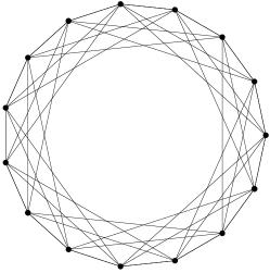
(a)

\psfrag{x}{$\gamma_{\max}$}\psfrag{b}{$\nu$}\psfrag{y}[b]{$\cfrac{(\sqrt{5}-1)\sqrt{\gamma_{\max}}+2(2\nu+1)}{2(\sqrt{5}-1)\sqrt{\gamma_{\max}}+2(2\nu+1)}$}\includegraphics[width=216.81pt]{figures/nu_gamma.eps}

(b)

Figure 3: On the left an example of Cayley graph $\mathcal{G}=(G,S)$ defined on the group $G=\mathds{Z}_{15}$ and $S=\{0,\pm 1,\pm 3,\pm 4\}$. On the right a plot that shows the first coefficient of (5.4) as function of $\gamma_{\max}$ and $\nu$ when the network topology is described by a Cayley graph. Furthermore, $\gamma_{\max}\in[0.5,1)$ and $\nu\in[0,10]$. As it can be seen, the coefficient is always less then one, and, compared to Figure 1, it depends only on $\nu$, namely the degree of a node and not on the network size $N$.

We have that each node communicates with $|S|-1=\nu$ nodes. In other words, two distinct nodes have in common at most $\nu$ nodes. This implies that $|\Theta_{\boldsymbol{\varphi}_{i}}|\leq 2\nu+1$. Thus

$$\sqrt{|\Theta_{\boldsymbol{\varphi}_{i}}|^{2}+4}-|\Theta_{\boldsymbol{\varphi}_{i}}|\geq(\sqrt{5}-1)/(2\nu+1)\,.$$

The first coefficient of (5.4) as function of $\gamma_{\max}$ and $\nu$ is shown in Figure 3b. Notice that the function is similar in shape to that in Figure 1, however in this case the dependence is on $\nu$, and not on the total number of nodes in the network $N$. Albeit the network might have a total number of nodes many orders of magnitude larger than $\nu$, the coefficient stays well below the one in (5.4), which has been obtained when no information about the network is known.

Since the coefficient of (5.4) is always much less than one, the designed estimator outperforms significantly the estimator that takes the average of the measurements.

6 Simulations and Numerical Results

Numerical simulations have been carried out to compare the estimator proposed in this paper with some related estimators available from the literature.

We consider the following five estimators:

${E_{1}}$:

${\bf K}(t)={\bf H}(t)=({\bf I}-\mathbf{L}(t))/2$ where $\mathbf{L}(t)$ is instantaneous Laplacian matrix associated to the graph $\mathcal{G}$. Clearly the graph changes when packets are dropped, so that arcs disappear from the graph.

${E_{2}}$:

${\bf K}(t)=\mathbf{0}$ and ${\bf H}(t)=[h_{ij}(t)]$ with $h_{ij}=1/|\mathcal{N}_{\boldsymbol{\varphi}_{i}}|$ if node $i$ and $j$ communicate, and $h_{ij}=0$ otherwise. Thus, the updated estimate is the average of the measurements (this is the estimator of Corollary 5.5).

${E_{3}}$:

${\bf K}(t)=[k_{ij}(t)]$, where $k_{ii}(t)=1/2|\mathcal{N}_{\boldsymbol{\varphi}_{i}}|$, $k_{ij}=1/|\mathcal{N}_{\boldsymbol{\varphi}_{i}}|$ if node $i$ and $j$ communicate, $k_{ij}(t)=0$ otherwise, whereas ${\bf H}(t)=[h_{ij}(t)]$ with $h_{ii}=1/2|\mathcal{N}_{\boldsymbol{\varphi}_{i}}|$, and $h_{ij}=0$ elsewhere. This is the average of the old estimates and node’s single measurement.

${E_{4}}$:

${\bf K}(t)={\bf H}(t)$ with $k_{ij}(t)=1/2|\mathcal{N}_{\boldsymbol{\varphi}_{i}}|$ if node $i$ and $j$ communicate, and $k_{ij}(t)=0$ otherwise. The updated estimate is the average of the old estimates and all local new measurements.

${E_{p}}$:

The estimator proposed in this paper.

The estimators $E_{1},\dots,E_{4}$ are based on various heuristics. They are related to proposals in the literature, e.g., ${E_{1}}$ uses filter coefficients given by the Laplacian matrix, cf., [10]–[12] and $E_{2}$ and $E_{3}$ are considered here as benchmark. Observe that the weights based on Laplacian do not ensure the minimization of the variance of the estimation error.

Figure 4 shows a set of test signals $d_{1}(t),\dots,d_{5}(t)$ that has been used to assess the various estimators. Note that the signals differ only in their frequency content. The test signals are highly nonlinear and generated so that the signal presents intervals in which is very slowly varying (low absolute value of the derivative) and intervals in which the derivative is higher.

\psfrag{d1}{$d_{1}(t)$}\psfrag{d2}{$d_{2}(t)$}\psfrag{d3}{$d_{3}(t)$}\psfrag{d4}{$d_{4}(t)$}\psfrag{d5}{$d_{5}(t)$}\includegraphics[width=346.89731pt]{figures/d_sig.eps}

Figure 4: Test signals used in the simulations. Signal $d_{2}(t),\dots,d_{5}(t)$ are obtained from $d_{1}(t)$ by changing the frequency. The test signals are highly nonlinear and are generated so that the signal shows intervals in which the derivative (in absolute value) is small and intervals in which the derivative is higher.

The choice of the parameter $\gamma_{\max}$ is based on the maximum cumulative bias, defined in Equation (3.5): Let $P_{b}$ denote the desired power of the cumulative biases of the estimates. Since there are $N$ nodes, we consider the average power of the bias of each node as $\Upsilon=P_{b}/N$. Assume that we want the estimator to guarantee that the power of the right-hand side of Equation (3.5) is equal to $\Upsilon$. This is equivalent to

$$\gamma_{\max}=\frac{\sqrt{\Upsilon}}{\sqrt{\Upsilon}+\Delta}\,.$$

In the simulations we have chosen $\Upsilon=0\>$dB, which is a rather low value, and the noise variance is $\sigma^{2}=1.5$, which is quite a large value if compared to the amplitude of the signal to track. We also assume that he value of $\Delta$ is not known precisely but with an upper bound of about $5$% from its real value. Therefore, these choices allow us to test the proposed estimator in the worst conditions.

We have considered 30 geometric random graphs with $N=20$ nodes uniformly distributed in a square of side length equal to $N/2$. Two nodes are connected if their Euclidean distance is less than $1.7\sqrt{N}$. The average neighborhood size of all the considered networks is $6.6$ nodes with a maximum and minimum neighborhood size of $11$ and $3$, respectively. The estimation of the test signals $d_{1}(t),\dots,d_{5}(t)$ has been performed under four different packet loss probabilities. More precisely we have consider the case in which $q_{ij}=0\%$, $q_{ij}=10\%\pm 5\%$, $q_{ij}=20\%\pm 5\%$ and $q_{ij}=30\%\pm 5\%$. We also considered different measurement noise realizations. We take the mean square error of the estimates of each node as performance measure. Each estimator has an initial transition phase, during which the mean square error may not be significant. Hence, it has been computed after $70$ steps. Afterwards, the mean square error has been averaged over all nodes of the network. The average is denoted by MSE. We define the improvement factor of our estimator compared to the estimators $E_{1},\ldots,E_{4}$ as

$$\chi_{i}=\frac{\text{MSE}({E_{i}})-\text{MSE}({E_{p}})}{\text{MSE}({E_{i}})}\,,\qquad i=1,\ldots,4\,.$$

Figure 5 shows the $\text{MSE}({E_{i}})$ for all the five different estimators as function of the packet loss probability. In the simulation we assume the nodes know the threshold value before the estimation process starts. This is typically achieved after 10 time steps and thus the network experiences a short initialization phase. Recall also that in all the simulations related to the proposed estimator $E_{p}$, the error covariance matrix is estimated at each node and reset as described in the end of Section 3.

\psfrag{X}[t]{Packet loss probability $q$}\psfrag{Y}[b]{MSE}\psfrag{T}{MSE for estimation of $d_{1}(t)$}\includegraphics[width=195.12767pt]{figures/signal05.eps}

(a)

\psfrag{X}[t]{Packet loss probability $q$}\psfrag{Y}[b]{MSE}\psfrag{T}{MSE for estimation of $d_{2}(t)$}\includegraphics[width=195.12767pt]{figures/signal10.eps}

(b)

\psfrag{X}[t]{Packet loss probability $q$}\psfrag{Y}[b]{MSE}\psfrag{T}{MSE for estimation of $d_{3}(t)$}\includegraphics[width=195.12767pt]{figures/signal15.eps}

(c)

\psfrag{X}[t]{Packet loss probability $q$}\psfrag{Y}[b]{MSE}\psfrag{T}{MSE for estimation of $d_{4}(t)$}\includegraphics[width=195.12767pt]{figures/signal35.eps}

(d)

\psfrag{X}[t]{Packet loss probability $q$}\psfrag{Y}[b]{MSE}\psfrag{T}{MSE for estimation of $d_{5}(t)$}\includegraphics[width=195.12767pt]{figures/signalconst.eps}

(e)

Figure 5: Mean Square Error (MSE) performance comparison among estimators for various packet loss probabilities $q$. Each plot is associated to one of the five test signals $d_{1}(t),\dots,d_{5}(t)$, see Figure 4. The marker $(\star)$ refers to $E_{1}$, $(\lozenge)$ refers to $E_{2}$, $(\square)$ refers to $E_{3}$, $(\bullet)$ refers to $E_{4}$ and $({\Large\triangleright})$ refers to the proposed estimator $E_{p}$. The vertical bars represent the variance of the MSE computed for the 30 simulations. Notice that the proposed estimator $E_{p}$ has a very low variance, thus showing its high robustness to packet loss and measurement noise.

Notice that $E_{p}$ outperforms all other estimators for any considered packet loss probability. The two estimators $E_{3}$ and $E_{4}$ have performance closer to $E_{p}$. In particular $E_{3}$ performs better when the signal is slow, whereas $E_{4}$ has better performance when the signal is faster. This is motivated by the fact that the estimator $E_{3}$ uses only one measurement and it is affected by a bias that depends on the derivative of signal $d(t)$ (see Figure 6). The $E_{3}$ performance improves as the packet loss probability increases. Indeed, the single local measurement is weighted more when packet losses occurs, i.e., previous estimates as lost, and thus the overall estimate becomes less biased. The other two heuristic estimators, $E_{2}$ and $E_{3}$, offer poor performance clearly in all the situations we have considered.

\psfrag{M}{Measurements}\psfrag{E1}{$E_{1}$}\psfrag{E2}{$E_{2}$}\psfrag{E3}{$E_{3}$}\psfrag{E4}{$E_{4}$}\psfrag{Ep}{$E_{p}$}\includegraphics[width=346.89731pt]{figures/curves.eps}

Figure 6: Realizations of the signal to be tracked, $d_{2}$, as it is measured by all the $N=20$ nodes, with a packet loss probability $q=10\%\pm 5\%$. Notice that the proposed estimator $E_{p}$, visibly outperforms all the other estimators in term of variance. Notice also that the proposed estimator presents a small bias when the signal changes more rapidly.

Figure 7 shows that the local computation of the weights ${\bf k}_{i}(t)$ with (3.9) yields a stable ${\bf K}(t)$. In particular, higher values of $\gamma({\bf K}(t))$ are experienced when the signal is slower, because $\Delta$ is small. Viceversa, lower values of $\gamma({\bf K}(t))$ are obtained when $\Delta$ is large. This is explained by considering that when the signal is slow, then it is better to weight more previous estimates (which means larger ${\bf K}(t)$ and hence larger $\gamma({\bf K}(t))$) to achieve small variances of the estimation error. By the same argument, when the signal is fast, then it is better to weight less previous estimates.

\psfrag{Y}{$\gamma(K(t))$}\psfrag{svdk1}{$\gamma(K(t))$ for $q=0.0$}\psfrag{svdk2}{$\gamma(K(t))$ for $q=0.1$}\psfrag{svdk3}{$\gamma(K(t))$ for $q=0.2$}\psfrag{svdk4}{$\gamma(K(t))$ for $q=0.3$}\psfrag{time step}{Time}\psfrag{a}[r]{\small{From $d_{5}$ to $d_{1}$}}\includegraphics[width=411.93767pt]{figures/svdk.eps}

Figure 7: Largest value of the singular value of the matrix ${\bf K}(t)$ in the 30 Monte Carlo simulation generated. The rows of ${\bf K}(t)$ are computed individually by each node using (3.9). The curves correspond to the five test signals $d_{1}(t),\dots,d_{5}(t)$, and they are ordered from the slowest signal ($d_{1}(t)$) to the fastest one ($d_{5}(t)$).

7 Conclusions and Future Work

In this paper, we presented a decentralized cooperative estimation algorithm for tracking a time-varying signal using a wireless sensor network with lossy communication. A mathematical framework was proposed to design a filter, which run locally in each node of the network. Performance analysis was carried out for the distributed estimation algorithm in time varying communication networks with packet loss probabilities both non-identical and identical among the links. losses. We investigated how the estimation quality depends on packet loss probability, network size and average number of neighboring nodes. The theoretical analysis showed that the filter is stable, and the variance of the estimation error is bounded even in the presence of large packet loss probabilities. Numerical results illustrated the validity of our approach, which outperforms other estimators available from the literature.

Future studies will be devoted to the extension of our design methodology to the case when models of the signal to track are available. Lossy communication links with memory will also be included. Furthermore, we plan to implement our distributed filter on real wireless sensor networks, thus experimentally checking the validity of our theoretical predictions.

8 Acknowledgments

We would like to thanks the anonymous reviewers for the very useful comments that allowed us to improve and strengthen the paper.

References

- [1] D. Estrin, R. Govindan, J. Eidemann, and S. Kumar, “Next century challenges: Scalable coordination in sensor networks,” in Proceedings of the ACM/IEEE International Conference on Mobile Computing and Networking, 1999.
- [2] H. Gharavi and P. R. Kumar, Eds., Proceedings of IEEE: Special Issue on Sensor Networks and Applications, vol. 91, 2003.
- [3] Z.-Q. Luo, M. Gatspar, J. Liu, and A. Swami, Eds., IEEE Signal Processing Magazine:Special Issue on Distributed Signal Processing in Sensor Networks. IEEE, 2006.
- [4] B. Aazhang, R. S. Blum, J. N. Laneman, K. J. R. Liu, W. Su, and W. A., Eds., Journal on Selected Areas in Communications: Cooperative Communication and Networking, vol. 25, no. 2, 2007.
- [5] A. Speranzon, C. Fischione, and K. H. Johansson, “Distributed and collaborative estimation over wireless sensor networks,” in IEEE Conference on Decision and Control, 2006.
- [6] ——, “A distributed estimation algorithm for tracking over wireless sensor networks,” in IEEE International Conference on Communication, 2007.
- [7] A. Jadbabaie, J. Lin, and A. S. Morse, “Coordination of groups of mobile autonomous agents using nearest neighbor rules,” IEEE Transactions on Automatic Control, vol. 48, no. 6, pp. 988–1001, 2003.
- [8] R. Olfati-Saber and R. M. Murray, “Consensus problems in networks of agents with switching topology and time-delays,” IEEE Transactions on Automatic Control, 2004.
- [9] R. Carli, F. Fagnani, A. Speranzon, and S. Zampieri, “Communication constraints in the average consensus problem,” Automatica, vol. 44, no. 3, 2008, to Appear.
- [10] L. Xiao, S. Boyd, and S. Lall, “A scheme for robust distributed sensor fusion based on average consensus,” In Proceedings of IEEE IPSN, 2005.
- [11] D. P. Spanos, R. Olfati-Saber, and R. M. Murray, “Approximate distributed Kalman filtering in sensor networks with quantifiable performance,” in IEEE Conference on Decision and Control, 2005.
- [12] R. Olfati-Saber and J. S. Shamma, “Consensus filters for sensor networks and distributed sensor fusion,” In Proceedings of IEEE Conference on Decision and Control, 2005.
- [13] L. Xiao, S. Boyd, and S. J. Kim, “Distributed average consensus with least-mean-square deviation,” Submitted to Journal of Parallel and Distributed Computing, 2006.
- [14] L. Xiao and S. Boyd, “Fast linear iterations for distributed averaging,” System Control Letter, 2004.
- [15] Y. Shang, W. Ruml, Y. Zhang, and M. Fromherz, “Localization from connectivity in sensor networks,” IEEE Transaction on Parallel and Distributed System, Vol. 15, No. 11, 2004.
- [16] A. Giridhar and P. R. Kumar, “Distributed clock synchronization over wireless networks: Algorithm and analysis,” in 45th IEEE Conference on Decision and Control, 2006.
- [17] R. Olfati-Saber, “Distributed kalman filtering for sensor networks,” in IEEE Conference on Decision and Control, 2007.
- [18] P. Alrikson and A. Rantzer, “Experimental evaluation of a distributed kalman filter algorithm,” in IEEE Conference on Decision and Control, 2007.
- [19] R. Carli, A. Chiuso, L. Schenato, and A. Zampieri, “Distributed kalman filtering using consensus strategies,” in IEEE Conference on Decision and Control, 2007.
- [20] A. Speranzon, C. Fischione, K. H. Johansson, and A. Sangiovanni-Vincentelli, “A distributed minimum variance estimator for sensor networks,” IEEE Journal on Selected Areas in Communications, Special Issue on Control and Communication, May 2008.
- [21] G. L. Stüber, Priciples of Mobile Communication. Kluwer Academic Publishers, 1996.
- [22] IEEE Std 802.15.4-2996, September, Part 15.4: Wireless Medium Access Control (MAC) and Physical Layer (PHY) Specifications for Low-Rate Wireless Personal Area Networks (WPANs), IEEE, 2006. [Online]. Available: http://www.ieee802.org/15
- [23] S. Boyd and L. Vandenberghe, Convex Optimization. Cambridge University Press, 2004.
- [24] M. Johansson and L. Xiao, “Cross-layer optimization of wireless networks using nonlinear column generation,” IEEE Transactions on Wireless Communications, vol. 5, February 2006.
- [25] R. Horst, P. M. Pardalos, and N. V. Thoai, Introduction to Global Optimization, Nonconvex Optimization and its Applications. Kluwer Academic Publisher, 1995.
- [26] D. P. Bertsekas and J. N. Tsitsiklis, Parallel and Distributed Computation: Numerical Methods. Athena Scientific, 1997.
- [27] M. T. Chao and W. E. Strawderman, “Negative moments of positive random variables,” Journal of the American Statistical Association, vol. 67, no. 388, 1972.
- [28] R. A. Horn and C. R. Johnson, Matrix Analysis. Cambridge University Press, 1985.