Quenches in quantum many-body systems: One-dimensional Bose-Hubbard model reexamined

Abstract

When a quantum many-body system undergoes a quench, the time-averaged density-matrix $\overline{\rho}$ governs the time-averaged expectation value of any observable. It is therefore the key object to look at when comparing results with equilibrium predictions. We show that the weights of $\overline{\rho}$ can be efficiently computed with Lanczos diagonalization for relatively large Hilbert spaces. As an application, we investigate the crossover from perturbative to non-perturbative quenches in the nonintegrable Bose-Hubbard model: on finite systems, an approximate Boltzmann distribution is observed for small quenches, while for larger ones the distributions do not follow standard equilibrium predictions. Studying thermodynamical features, such as the energy fluctuations and the entropy, show that $\overline{\rho}$ bears a memory of the initial state.

Recent experiments Experiments in ultra-cold atoms have renewed the interest for the time-evolution of an isolated quantum many-body system after a sudden change of the Hamiltonian parameters, the so-called “quantum quench”. Many questions arise from such a setup, among which are the relaxation to equilibrium statistics, the memory kept from the initial state, and the role of the integrability of the Hamiltonian. Analytical and numerical results support different answers to these questions Quenches ; Kollath2007 ; Manmana2007 ; Kollar2008 , though most of them have shown that observables do not follow usual equilibrium predictions. As it has been pointed out Kollar2008 ; Relaxation , looking at simple observables, yet experimentally accessible, might not be considered as sufficient to fully address these questions. Since time-evolution is unitary, there is no relaxation in the sense of a stationary density-matrix, contrary to what can happen in a subsystem Relaxation . However, observables will fluctuate with time around some average. Standard definitions show that the time-averaged density-matrix $\overline{\rho}$ of the system governs any observable and its fluctuations. It is therefore desirable to have a systematic way of getting some information about $\overline{\rho}$, and its associated thermodynamical-like quantities, in order to compare it with the density-matrices of equilibrium ensembles, such as the microcanonical or the canonical ensemble.

In this paper, we show how Lanczos diagonalization (LD) enables one to calculate the weights of the time-averaged density-matrix. This method, which gives access to relatively large Hilbert spaces, is helpful when an analytical calculation of the many-body wave-functions is lacking: this is, for instance, the case of nonintegrable models. As an application, the example of a quench in the one-dimensional Bose-Hubbard model (BHM) is revisited for the following reasons: (i) the model corresponds to realistic experiments Experiments , (ii) it is nonintegrable and it is usually believed that the redistribution of momenta through scattering causes thermalization, (iii) complementary numerical results already exist Kollath2007 , (iv) there is an equilibrium critical point demarcating two phases, and the latter can play a role in out-of-equilibrium physics. On finite systems, we show that there are two distinct regimes depending on the quench amplitude: in the perturbative regime, an approximate Boltzmann law is observed, while distributions which do not belong to equilibrium ensembles emerge for large quenches. Moreover, we show that the mixed state $\overline{\rho}$ bears some memory of the initial state through its energy fluctuations and its entropy.

We start by recalling Peres1984 and introducing some definitions. From now on, the discussion will be restricted to finite-size systems of length $L$ with no accidental degeneracy. We address the issue of the thermodynamical limit by looking at the scaling of observables with $L$, and by giving scaling arguments for the energy fluctuations. At time $t<0$, the Hamiltonian is denoted by $\mathcal{H}_{0}$ and its eigenvectors and eigenvalues by $\left|{\psi_{n}}\right\rangle$ and $E_{n}$. The system is prepared in some state $\left|{\psi_{0}}\right\rangle$, that usually is the ground-state of $\mathcal{H}_{0}$. At $t=0$, the Hamiltonian is changed to $\mathcal{H}$ which eigenvalues and eigenvectors are $\omega_{n}$ and $\left|{\phi_{n}}\right\rangle$. The time-evolving density-matrix of the whole system reads $\rho(t)=\sum_{n}p_{n}\left|{\phi_{n}}\right\rangle\left\langle{\phi_{n}}\right|+\sum_{n<m}\sqrt{p_{n}p_{m}}[e^{-i\Omega_{nm}t+i\Theta_{nm}}\left|{\phi_{n}}\right\rangle\left\langle{\phi_{m}}\right|+h.c.]$, with the relative phases $\Theta_{nm}=\theta_{n}-\theta_{m}$, using $\theta_{n}=\text{Arg}\left\langle{\phi_{n}}|{\psi_{0}}\right\rangle$, and the frequencies $\Omega_{nm}=\omega_{n}-\omega_{m}$. The $p_{n}=|{\left\langle{\psi_{0}}|{\phi_{n}}\right\rangle}|^{2}$ are the diagonal weights of the density-matrix, and they satisfy $\sum_{n}p_{n}=1$. As we are generally interested in the time-averaged expectation value of an observable $O$, we define $\overline{O}=\lim_{t\to\infty}\frac{1}{t}\int_{0}^{t}\text{Tr}[\rho(s)O]ds=\sum_{n}p_{n}O_{nn}$, with the matrix elements $O_{nm}=\left\langle{\phi_{n}}|{O}|{\phi_{m}}\right\rangle$. Interestingly, averaging $\langle{O}\rangle_{0}$ [with the notation $\langle{\cdot}\rangle_{0}=\left\langle{\psi_{0}}\right|\cdot\left|{\psi_{0}}\right\rangle$] over random initial phase differences $\Theta_{nm}$ gives back $\overline{O}$, relating the time-averaging to the loss of information on the initial phases. Similarly, by averaging $\rho(t)$ over time, one gets

$$\overline{\rho}=\sum_{n}p_{n}\left|{\phi_{n}}\right\rangle\left\langle{\phi_{n}}\right|\;,$$

which governs any time-averaged observable since $\overline{O}=\text{Tr}[\overline{\rho}O]$. Furthermore, it has been very recently shown Work that $\overline{\rho}$ is the experimentally relevant object to look at, and that the $p_{n}$ weights enter in the microscopic expression of the work and heat done on the system in the quench. Notice that the evolving state is a pure state so its von Neumann entropy $S[\rho]=-\text{Tr}[\rho\ln\rho]$ is zero, while $S[\overline{\rho}]$ is non-zero due to the loss of information induced by time-averaging. In addition, one must also look at the time-averaged fluctuations $\Delta O=[\text{Tr}[\overline{\rho}(O-\overline{O})^{2}]]^{1/2}$ of the observables. We finally mention that, if $O$ is diagonal in the $\left|{\phi_{n}}\right\rangle$ basis, like the energy $\mathcal{H}$, the time-averaged expectations and fluctuations are fixed by the initial state: $\overline{O}=\langle{O}\rangle_{0}$ and $\Delta O=[\langle{(O-\overline{O})^{2}}\rangle_{0}]^{1/2}$.

The difficulty for a given system is to compute the weights $p_{n}$ or any expectation value. When there is no analytical approach, as for the BHM, a possible solution is to resort to numerical techniques. In order to compute the $p_{n}$, we notice that they enter in the expression of the (squared) fidelity Peres1984 $F(t)=|{A(t)}|^{2}=1-4\sum_{n<m}p_{n}p_{m}\sin^{2}[\Omega_{nm}t/2]$. This is the revival probability after a time $t$ because we have $A(t)=\left\langle{\psi(t)}|{\psi_{0}}\right\rangle$, with $\left|{\psi(t)}\right\rangle$ the time-evolving wave-function. A direct time-evolution calculation usually fails after some time Kollath2007 . Our idea is to use spectral methods Dagotto1994 ; Mila1996 to get the Fourier transform $A(\omega)$ of the $A(t)$ function. Contrary to the approach of Ref. Mila1996, , we notice that LD also gives a direct access to the Lehmann representation $A(\omega)=\sum_{n}p_{n}\delta(\omega-\omega_{n}+E_{0})$ without a finite broadening, which induces an artificial decay of $A(t)$. Hence, all the information we need to discuss the statistical features of $\overline{\rho}$ is included in $A(\omega)$, since both the energies and the weights are obtained. LD is not an exact method but is well adapted to low-energies, i.e. long times, and we give below a perturbative argument corroborating that the $p_{n}$ have an overall decrease with $\omega_{n}$ [see also EPAPS for cross-checking]. Hilbert spaces of sizes up to $10^{7}$ states will be studied in the following while our full diagonalizations are restricted to $5000$ states. Lastly, spectral methods being much faster than time-evolution ones, one can scan a wide range of parameters.

The short and long time behaviors of $F(t)$ also contain information about the $p_{n}$ distribution Peres1984 : at short times $F(t)\simeq 1-t^{2}/\tau^{2}$ with $\tau^{-1}=\Delta E$, the energy fluctuations. Physically, the typical time $\tau$ is the time after which the system has “escaped” from the initial state, and is the inverse of the centered width of $A(\omega)$. More generally, higher moments of the $A(\omega)$ function are defined by $M_{q}=\langle{[\mathcal{H}-\langle{\mathcal{H}}\rangle_{0}]^{q}}\rangle_{0}$, and are clearly fixed by the initial state. In practice, the moments can also be independently computed with LD for $q$ up to hundred by iteratively applying $\mathcal{H}$ on $\left|{\psi_{0}}\right\rangle$. The associated sum rules are useful to cross-check the calculation of the spectrum. If one understands $A(\omega)$ as a probability distribution, knowing all moments amounts to knowing the distribution itself and would give back the exact $\overline{\rho}$. This comment was put forward without proof in Ref. Manmana2007, , together with a relevant discussion on the relation between these moments and generalized Gibbs ensembles. At long times, $F(t)$ usually fluctuates around its mean value $\bar{F}=\sum_{n}p_{n}^{2}$ Peres1984 . A qualitative interpretation of $\bar{F}$ is the “participation ratio” Peres1984 that counts the number of eigenstates which contributes to time evolution. The typical fluctuations of the fidelity are $(\Delta F)^{2}=\overline{F(t)^{2}-\bar{F}^{2}}=4\sum_{n<m}p_{n}^{2}p_{m}^{2}$. This quantity measures the strength of the wavering of the evolving state between getting back to $\left|{\psi_{0}}\right\rangle$ or getting away from $\left|{\psi_{0}}\right\rangle$.

Qualitatively, a quench consists in projecting the initial state onto the spectrum of the Hamiltonian $\mathcal{H}$ governing the dynamics. Straightforward results from perturbation theory in the quench amplitude illustrate the difference between small and large quenches: one expects a crossover between the two regimes. Writing $\mathcal{H}=\mathcal{H}_{0}+\lambda\mathcal{H}_{1}$ with $\lambda$ the quench amplitude and $\mathcal{H}_{1}$ the perturbing operator, the perturbed weights read, for $\lambda\ll 1$, $p_{0}\simeq 1-\lambda^{2}\sum_{n\neq 0}h_{n0}$, and $p_{n\neq 0}\simeq\lambda^{2}h_{n0}$, in which the notation $h_{n0}=|{\left\langle{\psi_{n}}|{\mathcal{H}_{1}}|{\psi_{0}}\right\rangle}|^{2}/(E_{n}-E_{0})^{2}$ has been used. Meanwhile, the $\omega_{n}$ are slightly shifted to order $\lambda$ and the eigenfunctions too. Thus, the $p_{n}$ have an overall decrease with the excited energy and, increasing $\lambda$ induces a transfer of spectral weight from the “targeted” ground-state $\left|{\phi_{0}}\right\rangle$ to other excited states. We get the scaling of several quantities to lowest order in $\lambda$: $M_{q}\propto\lambda^{2}$, $1-\bar{F}\propto\lambda^{2}$ and $\Delta F\propto\lambda^{2}$. As $\bar{F}>0$, these scalings will naturally fail for large $\lambda$, signaling the crossover to the non-perturbative regime. In addition, we mention that the mean-energy $\langle{E}\rangle$ is simply always linear in $\lambda$, since we have $\langle{E}\rangle=\langle{\mathcal{H}}\rangle_{0}=E_{0}+\lambda\langle{\mathcal{H}_{1}}\rangle_{0}$.

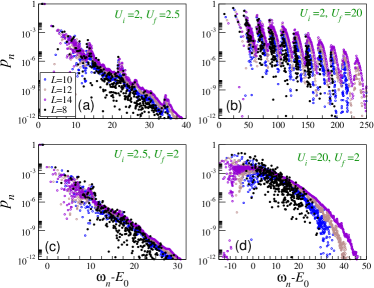
Figure 1: (Color online) Distributions of the $p_{n}$ at four different points of the $(U_{i},U_{f})$ state diagram. For the smallest size $L=8$, exact results are obtained by full diagonalization.

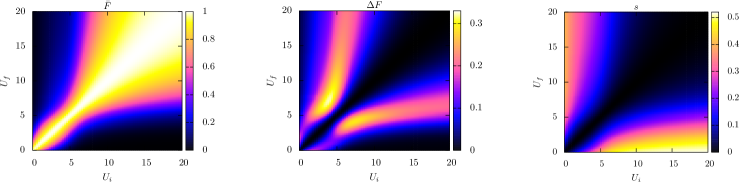
Figure 2: (Color online) Maps of the observables $\bar{F}$, $\Delta F$ and entropy per particle $s$ characterizing the time-averaged density-matrix $\overline{\rho}$. Results are obtained by LD on a finite system ($L=12$) with periodic boundary conditions.

Application to a quench in the one-dimensional Bose-Hubbard model – We now study the BHM in a one-dimensional optical lattice which is a nonintegrable model:

$$\mathcal{H}=-J\sum_{j}[b^{{\dagger}}_{j+1}b_{j}+b^{{\dagger}}_{j}b_{j+1}]+U/2\sum_{j}n_{j}(n_{j}-1)\,,$$

with $b^{{\dagger}}_{j}$ the operator creating a boson at site $j$ and $n_{j}=b^{{\dagger}}_{j}b_{j}$ the local density. $J$ is the kinetic energy scale while $U$ is the magnitude of the onsite repulsion. In an optical lattice, the ratio $U/J$ can be tuned by changing the depth of the lattice and using Feshbach resonance Experiments . When the density of bosons is fixed at $n=1$ and $U$ is increased, the equilibrium phase diagram of the model displays a quantum phase transition from a superfluid phase to a Mott insulating phase in which particles are localized on each site. The critical point has been located at $U_{c}\simeq 3.3J$ using numerics Kuhner2000 . The quenches are performed by changing the interaction parameter $U_{i}\rightarrow U_{f}$ (we set $J=1$ in the following), so we have $\lambda=(U_{f}-U_{i})/2$, and the perturbing operator $\mathcal{H}_{1}=\sum_{j}n_{j}(n_{j}-1)$ is diagonal. Numerically, one must fix a maximum onsite occupancy. We take four as in Ref. Kollath2007, (for further details, see EPAPS ).

Since $\overline{\rho}$ features a mixed state, we call the $(U_{i},U_{f})$ plane a state diagram. The $U_{i}=U_{f}$ ($\lambda=0$) line splits this state diagram in two regions and the previous perturbative arguments should hold close to this line. The typical distributions of the weights versus energy for four points of the state diagram are given in Fig. 1: two (a,c) with small quenches with parameters of the same (superfluid) equilibrium phase, and two (b,d) with large quenches, in which $U_{f}$ “crosses” $U_{c}$ in both directions. We observe that in the first two situations, for small $\lambda$, the distributions are close to an exponential decay typical of a canonical ensemble. This result supports the evidence of a “thermalized” regime as found in Ref. Kollath2007, , but on more general grounds since we directly have the distribution. Secondary peaks in Fig. 1(a) yield correction to this Boltzmann law. By looking at the cases of large quenches, we see that the distributions are strongly different from either the microcanonical or the canonical ensemble. When $U_{f}=20$ [Fig. 1(b)], Mott excitations, corresponding to doubly occupied sites and roughly separated by $U_{f}$, are clearly visible in the spectrum. Although the overall decay of the $p_{n}$ is exponential, the distribution is very different from a Boltzmann law. This explains that many observables differ from the ones of an equilibrium system, and independently corroborates results of Ref. Kollath2007, . When $U_{f}=2$ [Fig. 1(d)], the targeted spectrum is nearly continuous and the distribution displays large weights around zero energy and a subexponential-like behavior [approximately $\exp(-(\omega_{n}-E_{0})^{\gamma})$ with $\gamma>1$]. This is again different from equilibrium predictions. The bump-like shape of the $U_{f}=2$ distribution can be qualitatively understood from the fact that the ground-state energy increases with $U$ in the BHM. As $E_{0}>\omega_{0}$ when $U_{f}<U_{i}$, the initial state is close in energy to some excited states of $\mathcal{H}$ and, according to the perturbative form of the $p_{n}$, this favors their excitations by the quenching process. Another consequence is that the state diagram is expected to be non-symmetrical with respect to the $U_{i}=U_{f}$ line.

Crossover and finite size effects – To sketch the state diagram, maps of integrated quantities such as $\bar{F}$, $\Delta F$, and the entropy per particle $s=S[\overline{\rho}]/N$ are computed on a finite system with $L=12$ and given in Fig. 2. The normalization of the entropy $S[\overline{\rho}]$ is motivated by the fact that we observe that it scales as $N$, plus some finite-size corrections. As suggested previously, observables display a crossover from the perturbative regime to a non-perturbative regime characterized by a significant enhancement of the weights of excited states. In order to evaluate the finite size effects on the crossover, we look at the scalings of $\bar{F}$ and $\Delta F$ for a cut along the $U_{i}=2$ line and increasing $\lambda$. A first question is how the size of the perturbating regime evolves when increasing the length $L$. To address this question, we look at the evolution of two demarcating points. One is associated with $\bar{F}$ and is inconclusive (for further details, see EPAPS ). More interestingly, $\Delta F$ scales as $\lambda^{2}$ in the perturbative regime and the slope increases with $L$ (see Fig. 3). At large $\lambda$, $\Delta F$ is nearly flat and rapidly decreases with $L$. In between, it passes through a maximum that defines a demarcating point $\lambda_{c}(L)$, and the corresponding $\Delta{F}_{c}=\Delta{F}(\lambda_{c}(L))$. The scaling of $\lambda_{c}(L)$ suggests a finite value in the thermodynamical limit [see Fig. 3(c)]. $\Delta{F}_{c}$ can scale to a finite value but also to zero as a power-law [see Fig. 3(b)]. We notice that the latter situation would be in contradiction with a finite $\lambda_{c}$ and the fact that $\Delta F$ increases with $L$ at low $\lambda$. These results suggest that the perturbative regime survives in the thermodynamical limit, but they remain questionable. From the extrapolations, we find that the crossover survives for larger sizes, and could be experimentally relevant since experiments deal with finite systems. Notice that some of the numerics in Ref. Kollath2007, were done on larger systems. Another question one can ask is the role of the critical point on the observed maximum of the fluctuations of the fidelity: one may define the “equilibrium expectation” $\lambda_{c}^{eq}=(U_{c}-U_{i})/2$ [resp. $(U_{f}-U_{c})/2$] if one scans over $U_{f}$ [resp. $U_{i}$] and compare it with the scalings of actual $\lambda_{c}$. In Fig. 3(c), the two are too close to be conclusive but for large $U_{i,f}$ EPAPS , the difference is much substantial and $\lambda_{c}(L)$ even scales away from $\lambda_{c}^{eq}$. Thus, we infer that $U_{c}$ certainly plays a role (see below and Fig. 4), but not on the crossover nor on the location of $\Delta{F}_{c}$.

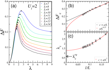
Figure 3: (Color online) (a) Cut along the $U_{i}=2$ line showing a maximum of $\Delta{F}$ between the perturbative and non-perturbative regimes of the quench. (b-c) Finite size scalings of $\Delta{F}_{c}$ and $\lambda_{c}$. See text for discussion.

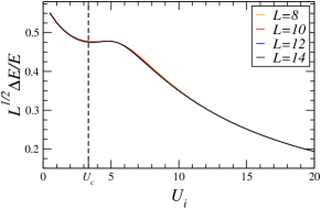
Figure 4: (Color online) Rescaled relative energy fluctuations in the mixed state. They only depend on the features of the initial state. The slope of the curves vanishes close to the equilibrium critical point $U_{c}$.

We now discuss some of the thermodynamical features of the mixed states described by the density-matrix $\overline{\rho}$. Firstly, we ask whether the averaged energy is well-defined by looking at the relative energy fluctuations defined as $\Delta E/E\equiv\Delta E/(\langle{E}\rangle-E_{0}+\lambda N)=\sqrt{\sum_{ij}\langle{n_{i}^{2}n_{j}^{2}}\rangle_{0}-\langle{n_{i}^{2}}\rangle_{0}\langle{n_{j}^{2}}\rangle_{0}}/\sum_{i}\langle{n_{i}^{2}}\rangle_{0}$ to get rid of the obvious dependencies of $\langle{E}\rangle$ on $E_{0}$, $N$ and $\lambda$: what remains are the relative “squared density” fluctuations in the initial state. In the superfluid phase, we expect Giamarchi2004 the squared density-density correlations to have an asymptotic algebraic behavior $\langle{n^{2}_{i}n^{2}_{j}}\rangle_{0}-\langle{n^{2}_{i}}\rangle_{0}\langle{n^{2}_{j}}\rangle_{0}\sim|i-j|^{-\alpha}$, while they should be exponential in the Mott phase $e^{-|i-j|/\xi}$, with $\xi$ the correlation length. On a chain of length $L$, we thus have $\Delta E=\lambda\sqrt{L}g(L)$ with: (i) if $\alpha<1$, then $g(L)\sim L^{(1-\alpha)/2}$, (ii) if $\alpha=1$, $g(L)\sim\sqrt{\ln L}$ and if $\alpha>1$ or $\xi>0$, $g(L)=\text{const}$. As we have $\alpha>1$ in the superfluid phase of the 1D BHM Giamarchi2004 and $\sum_{i}\langle{n_{i}^{2}}\rangle_{0}\sim L$, we find that $\Delta E/E=f(U_{i},L)/\sqrt{L}$ for any $U_{i}$. The $f(U_{i},L)$ function is computed with LD and plotted in Fig. 4. It shows a very good agreement with this scaling argument since $f$ hardly depends on $L$. This $1/\sqrt{L}$ scaling resembles the ones of the (micro)canonical ensembles but, one also notices that starting from a initial state with strong density fluctuations ($\alpha\leq 1$) leads to anomalous scalings of the relative energy fluctuations. In the BHM, this could be achieved by introducing nearest neighbor repulsion Kuhner2000 . We also get the scaling of the typical time $\tau\sim\lambda^{-1}L^{-1/2}$. This shows that, even if $\tau$ scales to zero in the thermodynamical limit, it can be significantly long on large but finite systems for small $\lambda$. More importantly, we find that two mixed states $\overline{\rho}$ can have the same energy $\langle{E}\rangle$ but with different $\lambda$, since $\langle{E}\rangle=E_{0}+\lambda\langle{\mathcal{H}_{1}}\rangle_{0}$. Hence, each of them originates from a different initial state and consequently, the two states have different energy fluctuations. Consequently, $\overline{\rho}$ keeps a memory on the initial state. Another important thermodynamical feature is the entropy per particle $s$ that continuously increases with $\lambda$ and reveals more significantly the underlying anisotropy of the state diagram [see Fig. 2]. We have checked that two mixed states with the same mean energy $\langle{E}\rangle$ have different entropies, so $\overline{\rho}$ also keeps a memory of the initial state through its entropy. From the very definition of the $p_{n}$, this is not surprising.

In conclusion, we have shown that the weights of the time-averaged density-matrix $\overline{\rho}$ can be obtained with LD. This provides an observable-free description of the quench process, in particular for nonintegrable models. The method is applied to the 1D BHM where it is shown that, on finite systems, there is a clear crossover from a perturbative regime, in which the distribution is Boltzmann-like in the superfluid region, to distributions that are not predicted by equilibrium statistics ensembles. The state diagram has been mapped out in the $(U_{i},U_{f})$ plane and finite size effects have been investigated. Lastly, we showed that the mixed state $\overline{\rho}$ has a well-defined energy and that it keeps a memory of the initial state through its energy fluctuations or its entropy.

I thank T. Barthel, F. Heidrich-Meisner, T. Jolicoeur, D. Poilblanc and D. Ullmo for fruitful discussions.

Electronic physics auxiliary publication service for: On quenches in quantum many-body systems: the one-dimensional Bose-Hubbard model revisited

Typical behavior of the fidelity with time

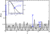
Figure 5: Typical behavior of the fidelity for a finite size system with $L=10$ starting from $U_{i}=2$ to $U_{f}=8$ ($\lambda=3$). At short times: $F(t)=1-t^{2}/\tau^{2}$ (here $\tau=0.14$). For long times, $F(t)$ fluctuates around its mean value $\bar{F}$ (here $\bar{F}=0.135$ and $\Delta F=0.136$).

Technical details on Lanczos calculations

We use 200 Lanczos iterations to get the ground state and 1200 to get the Lehmann representation of $A(\omega)$. We do not use symmetries of the Hamiltonian except particle number conservation. With periodic boundary conditions, translational symmetries induce some selection rules for the $p_{n}$ so their number is quite reduced. We have checked that Lanczos gives a good result by comparing it with exact results obtained by full diagonalization on a system with $L=8$ (see Fig. 6. The largest Hilbert space size is 13311000 for $L=14$ for Lanczos diagonalization and 5475 for $L=8$ for full diagonalization. Very similar results are obtained from systems with open boundary conditions.

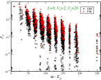
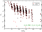
Figure 6: Test on symmetries and effect of boundary conditions on the distribution of the $p_{n}$. PBC stands for periodic boundary conditions while OBC is for open BC.

Additional results on the Bose-Hubbard model

Moments are related to the $p_{n}$ and $\omega_{n}$ through $M_{q}=\sum_{n}p_{n}[\omega_{n}-\langle{E}\rangle]^{q}$. They undergo a clear change of behavior with increasing $\lambda$ as shown in Fig. 7.

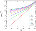
Figure 7: First moments $M_{q}$ (to the power $1/q$) of the $A(\omega)$ function for a system with $L=10$ and $U_{i}=2$. There is a crossover from the perturbative result $M_{q}\sim\lambda^{2}$ (gray lines) to a regime where $M_{q}\sim\lambda^{q}$ at large $\lambda$.

We give below the behavior of $\bar{F}$ which goes from 1 when $\lambda=0$ to small value when $\lambda$ is large. On a finite system, the second derivative $d^{2}\bar{F}/d\lambda^{2}$ crosses zero for a value $\lambda_{c}(L)$ and we define the corresponding $\bar{F}_{c}=\bar{F}(\lambda_{c}(L))$. The scalings with $1/L$ of these two quantities are given in Fig. 8: a linear scaling suggests that they are finite in the thermodynamical limit but power-law scalings going to zero also works for both, so studying this quantity is not very conclusive. Power-law scalings are however very slow, which means that even for large systems of length 100 or 1000 (experimentally relevant), the perturbative regime should survive.

Notice that in the three other cuts of $\Delta F$ [Fig. 8] support that the same increase of $\Delta F$ with $L$ in the perturbative regime as for the $U_{i}=2$ case of the paper.

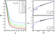
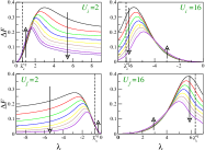
Figure 8: Left: Cut along the $U_{i}=2$ axis of $\bar{F}$. A linear scaling gives both a finite value for $\bar{F}_{c}$ and $\lambda_{c}$ but a power-law one (going to zero) is also plausible. Right: Four cuts in the state diagram showing the scaling behavior of $\Delta F(L)$ as a function of $\lambda$. The smallest size is $L=6$ and larger $L=13$ except for $U_{i}=2$ for which it is $L=14$. Results for $L=6,7,8$ are exact (full diagonalization) while larger sizes are obtained with Lanczos. The arrows indicate how $\Delta F$ increases or decreases with $L$.

References

- (1) M. Greiner, O. Mandel, T. W. Hänsch, and I. Bloch, Nature 419, 51 (2002); T. Kinoshita, T. Wenger, and D. S. Weiss, Ibid. 440, 900 (2006); S. Hofferberth, I. Lesanovsky, B. Fischer, T. Schumm, and J. Schmiedmayer, Ibid. 449, 324 (2007).
- (2) R. Schützhold, M. Uhlmann, Y. Xu, and U. R. Fischer, Phys. Rev. Lett. 97, 200601 (2006); M. A. Cazalilla, Ibid. 97, 156403 (2006); P. Calabrese and J. Cardy, Ibid. 96, 136801 (2006); M. Rigol, V. Dunjko, V. Yurovsky, and M. Olshanii, Ibid. 98, 050405 (2007); M. Eckstein and M. Kollar, Ibid. 100, 120404 (2008); M. Möckel and S. Kehrein, Ibid. 100, 175702 (2008); F. Heidrich-Meisner, M. Rigol, A. Muramatsu, A. E. Feiguin, and E. Dagotto, Phys. Rev. A 78, 013620 (2008); M. Rigol, V. Dunjko, and M. Olshanii, Nature 452, 854 (2008);
- (3) C. Kollath, A. M. Läuchli, and E. Altman, Phys. Rev. Lett. 98, 180601 (2007).
- (4) S. R. Manmana, S. Wessel, R. M. Noack, and A. Muramatsu, Phys. Rev. Lett. 98, 210405 (2007).
- (5) M. Kollar and M. Eckstein, Phys. Rev. A 78, 013626 (2008).
- (6) M. Cramer, C. M. Dawson, J. Eisert, and T. J. Osborne, Phys. Rev. Lett. 100, 030602 (2008); T. Barthel and U. Schollwöck, Ibid. 100, 100601 (2008); M. Cramer, A. Flesch, I. P. McCulloch, U. Schollwöck, and J. Eisert, Ibid. 101, 063001 (2008).
- (7) A. Peres, Phys. Rev. A 30, 1610 (1984); Ibid. 30, 504 (1984).
- (8) A. Silva, Phys. Rev. Lett. 101, 120603 (2008); A. Polkonikov, preprint, arXiv:0806.0620; P. Reimann, preprint, arXiv:0810.3092.
- (9) E. Dagotto, Rev. Mod. Phys. 66, 763 (1994).
- (10) F. Mila and D. Poilblanc, Phys. Rev. Lett. 76, 287 (1996).
- (11) See the EPAPS file online.
- (12) T. D. Kühner, S. R. White, and H. Monien, Phys. Rev. B 61, 12474 (2000).
- (13) T. Giamarchi, Quantum Physics in One Dimension (Oxford University Press, Oxford 2004).