Multiple charge spreading as a generalization of the Bertaut approach to lattice summation of Coulomb series in crystals

Abstract

The Bertaut approach associated with charge spreading so as to enhance the rate of convergence of Coulomb series in crystals is extended to the case of an arbitrary multiple spreading with a given initial spreading function. It is shown that the effect of spreading may in general be treated as a uniform transformation of space, providing that zero mean potential as a universal spatial property is sustained. As a result, electrostatic potentials driven by different orders of multiple spreading can be obtained from the same energy functional in a consistent manner. It is found that the effect of multiple spreading gives rise to more advanced forms described, for example, by simple exponential decrease, but the functional description based on a Gaussian spreading turns out to be invariant. In addition, the effects of a multiple charge spreading based on simple exponential and Gaussian spreading functions are compared as typical of molecular calculations.

1 Introduction

The problem of lattice summation of Coulomb series over crystal structures is principal for describing solid state. Apart from a large number of traditional approaches to this subject [1, 2, 3], many novel proposals for solving this problem still arise [4, 5, 6, 7, 8, 9, 10, 11, 12]. Nevertheless, the classical Ewald approach [13] remains one of the most effective and so widespread [14, 15, 16, 17]. This is the reason that understanding the nature of this efficiency is of great importance [18]. In particular, its relation to the effect of screening Coulomb potentials was revealed by Nijboer and De Wette [19]. As a result, some generalizations associated with different types of screening have been proposed [16, 20]. Another fruitful explanation of the foregoing efficiency is based on the idea of charge spreading proposed first by Ewald in his original paper [13] and developed further by Bertaut [21]. In particular, this generalized approach turns out to be expedient in applications to molecular dynamics [16, 22]. Here we will discuss this treatment in more amount of detail so as to coincide known variations inherent in its implementation.

In the original paper of Bertaut [21] the pair-wise Coulomb interaction is discussed. As a result, the double charge spreading naturally arises in that approach. In particular, this feature results in the fact that the square of the Fourier transform describing the spreading function takes place in the sum over the reciprocal lattice contributing to the Coulomb energy [21, 23]. On the other hand, it turns out that a single charge spreading is still sufficient if the electrostatic potential is first considered [24, 25, 26]. As a result, the Fourier transform of the spreading function, but not its square, arises in the sum over reciprocal lattice vectors contributing to the energy within such a treatment. This fact was the subject of discussion [25, 27, 28]. Altogether, it was shown that both the treatments are quite correct and can eventually originate the description proposed by Bertaut. Nevertheless, the original treatment proposed by Bertaut appears to be symmetric with respect to both the set of charges generating potentials and the similar set of charges interacting with those potentials. It is instructive that the latter situation may be regarded as some uniform transformation of space [3, 22].

In the present paper we extend the concept of charge spreading and introduce the regular idea of a multiple spreading, bearing in mind that this effect can always be addressed to the charge distribution generating the potential field. On the other hand, such a standpoint is not obviously unique and therefore various other points of view are discussed. In particular, the idea of spreading as a uniform transformation of space is developed in a general form. In addition, in the case of a multiple spreading the universal character of the Ewald approach is recognized. The effect of a multiple charge spreading on the Coulomb interaction between a couple of objects neutral on average is also discussed.

2 Preliminaries

Let us consider a crystal described by a charge distribution $\rho_{\rm{c}}({\bi{r}})$ subject to translational symmetry. On the other hand, we can also introduce a local charge distribution $\rho({\bi{r}})$ attributed to a unit cell and driven by the natural condition of electrical neutrality

$$\int_{V}\rho({\bi{r}})\,d{\bi{r}}=0,$$ (1)

where the integration is carried out over a volume $V$ occupied by $\rho({\bi{r}})$. Note that the unit-cell parallelepiped of volume $v$, constituted of three noncomplanar vectors of elementary translations of a Bravais lattice at hand, is assumed to be contained completely in $V$. The latter is essential if $\rho({\bi{r}})$ is spread beyond that parallelepiped volume [3]. Then the overall charge distribution in question can be written as

$$\rho_{\rm{c}}({\bi{r}})=\sum_{i}\rho({\bi{r}}-{{\bi{R}}_{i}}),$$ (2)

where the summation over $i$ is performed over sites specified by vectors ${{\bi{R}}_{i}}$ appropriate to the Bravais lattice of interest. It is evident that representation (2) for $\rho_{\rm{c}}({\bi{r}})$ is not unique due to an optional choice of $\rho({\bi{r}})$ [3]. Nevertheless, form (2) is subject to translational symmetry as well. This is the reason that $\rho_{\rm{c}}({\bi{r}})$ defined by (2) can be cast in terms of a series over reciprocal lattice vectors ${\bi{h}}$:

$$\rho_{\rm{c}}({\bi{r}})=\mathop{{\sum}^{\prime}}_{\bi{h}}F({\bi{h}})\exp(2\pi i{\bi{h}}{\bi{r}}),$$ (3)

where the prime on the summation sign implies that the contribution of ${\bi{h}}=0$ is actually omitted, as follows from formula (7) derived later on. The structure factor $F({\bi{h}})$, by definition, is determined as [22, 28]

$$F({\bi{h}})=\frac{1}{v}\int_{\rm{cell}}\rho_{\rm{c}}({\bi{r}})\exp(-2\pi i{\bi{h}}{\bi{r}})\,d{\bi{r}}.$$ (4)

Here the integration is carried out over the unit-cell parallelepiped mentioned above. Substituting (2) into (4), we obtain

$$F({\bi{h}})=\frac{1}{v}\int_{\rm{cell}}d{\bi{r}}\sum_{i}\rho({\bi{r}}-{{\bi{R}}_{i}})\exp(-2\pi i{\bi{h}}({\bi{r}}-{{\bi{R}}_{i}})).$$ (5)

Bearing in mind that the integration over the unit-cell parallelepiped along with the summation over $i$ is transformed into the integration over all space [29] reduced eventually to $V$ intrinsic to $\rho({\bi{r}})$, relation (5) is converted into

$$F({\bi{h}})=\frac{1}{v}\int_{V}\rho({\bi{r}})\exp(-2\pi i{\bi{h}}{\bi{r}})\,d{\bi{r}}.$$ (6)

It is important that

$$F({\bi{h}}=0)=0,$$ (7)

in agreement with (1).

The electrostatic potential exerted by charge distribution (2) at a reference point ${\bi{r}}$ is of the form

$$U({\bi{r}})=\mathop{{\int}^{\prime}}\frac{\rho_{\rm{c}}({\bi{r}}_{1})\,d{\bi{r}}_{1}}{|{\bi{r}}_{1}-{\bi{r}}|},$$ (8)

where the prime on the integral sign stands for missing a singular contribution of any point charge if it happens at ${\bi{r}}$. If we now make use of Poisson’s equation for the Green function

$$\nabla^{2}_{\bi{r}}\frac{1}{|{\bi{r}}_{1}-{\bi{r}}|}=-4\pi\delta({\bi{r}}_{1}-{\bi{r}}),$$ (9)

where the differentiation is performed with respect to ${\bi{r}}$ and $\delta({\bi{r}})$ is the Dirac delta function, we readily confirm from (8) that $U({\bi{r}})$ is subject to the conventional Poisson’s equation of the form

$$\nabla^{2}_{\bi{r}}U({\bi{r}})=-4\pi\rho_{\rm{c}}({\bi{r}}).$$ (10)

On the other hand, on inserting (3) into (8), the result can be written as

$$U({\bi{r}})=\Bigl{[}\mathop{{\sum}^{\prime}}_{\bi{h}}F({\bi{h}})\int\frac{\exp(2\pi i{\bi{h}}{\bi{r}}_{1})\,d{\bi{r}}_{1}}{|{\bi{r}}_{1}-{\bi{r}}|}\Bigr{]}^{\prime},$$ (11)

where the square brackets decorated by the prime imply missing the same singular term mentioned in (8). It is easy to show that

$$\int\frac{\exp(2\pi i{\bi{h}}{\bi{r}}_{1})\,d{\bi{r}}_{1}}{|{\bi{r}}_{1}|}=\frac{1}{\pi|{\bi{h}}|^{2}}.$$ (12)

Substituting (12) into (11), we obtain

$$U({\bi{r}})=\frac{1}{\pi}\Bigl{[}\mathop{{\sum}^{\prime}}_{\bi{h}}\frac{F({\bi{h}})}{|{\bi{h}}|^{2}}\exp(2\pi i{\bi{h}}{\bi{r}})\Bigr{]}^{\prime}.$$ (13)

However, if we insert relation (2) directly into (8), the result is as follows:

$$U({\bi{r}})=\mathop{{\int}^{\prime}}\frac{d{\bi{r}}_{1}}{|{\bi{r}}_{1}-{\bi{r}}|}\sum_{i}\rho({\bi{r}}_{1}-{{\bi{R}}_{i}}).$$ (14)

If we go over to a new variable of integration ${\bi{r}}^{\prime}={\bi{r}}_{1}-{{\bi{R}}_{i}}$ now, then

$$U({\bi{r}})=\mathop{{\sum}^{\prime}}_{i}^{*}\int_{V}\frac{\rho({\bi{r}}^{\prime})\,d{\bi{r}}^{\prime}}{|{\tilde{\bi{R}_{i}}}|},$$ (15)

where

$${\tilde{\bi{R}_{i}}}={{\bi{R}}_{i}}+{\bi{r}}^{\prime}-{\bi{r}},$$ (16)

the prime on the summation sign in (15) means that the singular contribution associated with a point charge at ${\bi{r}}$ must be still excluded. The asterisk over the summation sign points to the fact that the summation over large ${{\bi{R}}_{i}}$ is not yet defined properly in formula (15) so as to be consistent with the absence of the ${\bi{h}}=0$ contribution in expression (13).

This inconsistency is the essence of the conditional convergence of Coulomb series in crystals. It is especially pronounced in the particular case of point-charge lattices described by [25]

$$\rho({\bi{r}})=\sum_{j}q_{j}\delta({\bi{r}}-{\bi{b}}_{j}),$$ (17)

where the summation over $j$ is carried out over point charges $q_{j}$ belonging to a unit cell, located at positions ${\bi{b}}_{j}$ and governed by the condition

$$\sum_{j}q_{j}=0,$$ (18)

in agreement with (1). Substituting (17) into (6), we deduce

$$F({\bi{h}})=\frac{1}{v}\sum_{j}q_{j}\exp(-2\pi i{\bi{h}}{\bi{b}}_{j}).$$ (19)

If relation (19) is now inserted into (13) and relation (17) is inserted into (15), where equation (16) is taken into account, then we obtain

$$U({\bi{r}})=\frac{1}{\pi v}\Bigl{\{}\mathop{{\sum}^{\prime}}_{{\bi{h}},j}\frac{q_{j}}{|{\bi{h}}|^{2}}\exp[2\pi i{\bi{h}}({\bi{r}}-{\bi{b}}_{j})]\Bigr{\}}^{\prime}=\mathop{{\sum}^{\prime}}_{i}^{*}\sum_{j}\frac{q_{j}}{T_{ij}},$$ (20)

where

$$T_{ij}=|{{\bi{R}}_{i}}+{\bi{b}}_{j}-{\bi{r}}|.$$ (21)

Here the contribution of ${\bi{r}}={\bi{b}}_{j}$ is supposed to be excluded in the first relation on the right-hand side of (20) and the same contribution at ${{\bi{R}}_{i}}=0$ is to be excluded in the second issue. Both of the expressions in (20) describe the same potential by definition, so that the singularity associated with the contribution of large ${{\bi{R}}_{i}}$ must be resolved as it is prescribed by exclusion of the ${\bi{h}}=0$ term. However, even in this case the convergence of the sum over ${\bi{h}}$ is not fast for general ${\bi{r}}$ [30]. The event of ${\bi{r}}$ at which a point charge exists is an exclusion, where a compensating term enhancing the rate of convergence arises [31].

3 Multiple charge spreading

In order to enhance the rate of convergence of the series mentioned above, we extend the treatment of Bertaut [21] and define a modified unit-cell charge distribution as follows:

$$\tilde{\rho}^{(n)}({\bi{r}}) = \int\sigma(|{\bi{r}}-{\bi{r}}_{1}|)\sigma(|{\bi{r}}_{1}-{\bi{r}}_{2}|)\dots\sigma(|{\bi{r}}_{n-1}-{\bi{r}}_{n}|)$$ (22)

$${}\times\rho({\bi{r}}_{n})\,d{\bi{r}}_{1}\dots d{\bi{r}}_{n},$$

where $n$ identical functions $\sigma(|{\bi{r}}|)$ are introduced. These functions spread the actual charge at every point in a consecutive manner and are normalized by the condition

$$\int\sigma(|{\bi{r}}|)\,d{\bi{r}}=4\pi\int_{0}^{\infty}\sigma(r)r^{2}\,dr=1,$$ (23)

where $r=|{\bi{r}}|$. Like (2), the modified overall charge distribution in the crystal then takes the form

$$\tilde{\rho}^{(n)}_{\rm{c}}({\bi{r}})=\sum_{i}\tilde{\rho}^{(n)}({\bi{r}}-{{\bi{R}}_{i}}).$$ (24)

This value can in turn be cast in terms of the Fourier transforms associated with the reciprocal lattice vectors:

$$\tilde{\rho}^{(n)}_{\rm{c}}({\bi{r}})=\mathop{{\sum}^{\prime}}_{\bi{h}}\tilde{F}^{(n)}({\bi{h}})\exp(2\pi i{\bi{h}}{\bi{r}}),$$ (25)

$$\tilde{F}^{(n)}({\bi{h}})=\frac{1}{v}\int_{\rm{cell}}\tilde{\rho}^{(n)}_{\rm{c}}({\bi{r}}_{1})\exp(-2\pi i{\bi{h}}{\bi{r}}_{1})\,d{\bi{r}}_{1}.$$ (26)

Substituting (24) into (26), we obtain

$$\tilde{F}^{(n)}({\bi{h}}) = \frac{1}{v}\int d{\bi{r}}\exp(-2\pi i{\bi{h}}{\bi{r}})\int d{\bi{r}}_{1}\dots d{\bi{r}}_{n}\sigma(|{\bi{r}}-{\bi{r}}_{1}|)$$ (27)

$${}\times\sigma(|{\bi{r}}_{1}-{\bi{r}}_{2}|)\dots\sigma(|{\bi{r}}_{n-1}-{\bi{r}}_{n}|)\rho({\bi{r}}_{n}).$$

If we here go over to new variables of integration

$${\bi{r}}^{\prime}_{n-1}={\bi{r}}_{n-1}-{\bi{r}}_{n},\quad\dots,\quad{\bi{r}}^{\prime}_{1}={\bi{r}}_{1}-{\bi{r}}_{2},\quad{\bi{r}}^{\prime}={\bi{r}}-{\bi{r}}_{1},$$ (28)

keeping in mind that

$${\bi{r}}={\bi{r}}^{\prime}+{\bi{r}}^{\prime}_{1}+\dots+{\bi{r}}^{\prime}_{n-1}+{\bi{r}}_{n},$$ (29)

then it is easy to show that

$$\tilde{F}^{(n)}({\bi{h}})=F({\bi{h}})S^{n}({\bi{h}}).$$ (30)

Here the function $S({\bi{h}})$ is defined by the relation

$$S({\bi{h}})=\int\sigma(|{\bi{r}}|)\exp(-2\pi i{\bi{h}}{\bi{r}})\,d{\bi{r}},$$ (31)

with the evident properties

$$S({\bi{h}})=S(-{\bi{h}}),\qquad S(0)=1,$$ (32)

in agreement with formula (23).

The modified electrostatic potential appropriate to (24) is naturally equal to

$$\tilde{U}^{(n)}({\bi{r}})=\int\frac{\tilde{\rho}_{\rm{c}}^{(n)}({\bi{r}}_{1})\,d{\bi{r}}_{1}}{|{\bi{r}}_{1}-{\bi{r}}|}.$$ (33)

Indeed, the substitution of (9) into (33) yields Poisson’s equation

$$\nabla^{2}_{\bi{r}}\tilde{U}^{(n)}({\bi{r}})=-4\pi\tilde{\rho}_{\rm{c}}^{(n)}({\bi{r}}_{1})$$ (34)

associated with (22). Comparing (33) with (8) and taking relations (13) and (30) into account, we readily derive

$$\tilde{U}^{(n)}({\bi{r}})=\frac{1}{\pi}\mathop{{\sum}^{\prime}}_{\bi{h}}\frac{F({\bi{h}})S^{n}({\bi{h}})}{|{\bi{h}}|^{2}}\exp(2\pi i{\bi{h}}{\bi{r}}),$$ (35)

where any restriction associated with a point charge contribution is immaterial now due to the attenuation effect of $S({\bi{h}})$. This is a direct consequence of the fact that there are no point charges after transformation (22).

On the other hand, if we insert definition (22) into (33) and make use of relations (28) and (29), then we obtain

$$\tilde{U}^{(n)}({\bi{r}})=\sum_{i}^{*}\int_{V}\rho({\bi{r}}^{\prime}){\mathit{\Omega}}^{(n)}(|{\tilde{\bi{R}_{i}}}|)\,d{\bi{r}}^{\prime},$$ (36)

where definition (16) is utilized, the asterisk over the summation sign points out that the problem of remote ${{\bi{R}}_{i}}$ still exists in the present representation,

$${\mathit{\Omega}}^{(n)}(|{\bi{R}}|)=\int\frac{\sigma(|{\bi{r}}_{1}|)\dots\sigma(|{\bi{r}}_{n}|)\,d{\bi{r}}_{1}\dots d{\bi{r}}_{n}}{|{\bi{R}}+{\bi{r}}_{1}+\dots+{\bi{r}}_{n}|}.$$ (37)

To overcome the problem of remote ${{\bi{R}}_{i}}$, the initial electrostatic potential of interest can be rewritten in the form

$$U_{(n)}({\bi{r}})\equiv\tilde{U}^{(n)}({\bi{r}})+\Bigl{[}U({\bi{r}})-\tilde{U}^{(n)}({\bi{r}})\Bigr{]}.$$ (38)

If we now utilize result (35) for the first term on the right-hand side of formula (38) and employ (15), (16) and (36) for the remainder, we get

$$U_{(n)}({\bi{r}}) = \frac{1}{\pi}\mathop{{\sum}^{\prime}}_{\bi{h}}\frac{F({\bi{h}})S^{n}({\bi{h}})}{|{\bi{h}}|^{2}}\exp(2\pi i{\bi{h}}{\bi{r}})$$ (39)

$${}+\mathop{{\sum}^{\prime}}_{i}\int_{V}d{\bi{r}}^{\prime}\rho({\bi{r}}^{\prime})\frac{W^{(n)}(|{\tilde{\bi{R}_{i}}}|)}{|{\tilde{\bi{R}_{i}}}|}-\Bigl{\{}q_{j}{\mathit{\Omega}}^{(n)}(0)\Bigr{\}}_{{\bi{r}}={\bi{b}}_{j}}.$$

Here we introduce the following compact definition

$$\frac{W^{(n)}(R)}{R}=\frac{1}{R}-{\mathit{\Omega}}^{(n)}(R)$$ (40)

for the difference characteristic of the case. As a result, the asterisk over the summation sign can be omitted, because the summation over $i$ in (39) is now carried out in a consistent manner resolving the conditional convergence of this sum at large ${{\bi{R}}_{i}}$. On the other hand, the prime on the summation sign over $i$ in (39) stands for the omission of the singular contribution of a point charge, if it happens, provided that such a contribution would be described by the first term on the right-hand side of (40). Finally, the last term on the right-hand side of (39) describes the elimination of the same contribution from the regular part specified by ${\mathit{\Omega}}^{(n)}(R)$ in (40).

It is important that the convergence of the first term on the right-hand side of expression (39) is expected to be rather fast due to the effect of $S({\bi{h}})$ and the same is right for the direct sum in the remainder, in accord with [21], as will be discussed in more amount of detail in [32].

Note that in the case of $n=1$ result (39) is tantamount to the Nijboer-De Wette approach [19], bearing in mind that normalization (23) is not principal here due to the fact that this representation is after all incorporated by means of identity (38).

4 Charge spreading as a uniform transformation of space

It is important that the spreading at hand can be treated as a uniform transformation of space [3]. Indeed, according to (22), this transformation connecting an initial point ${\bi{r}}^{\prime}$ with a final point ${\bi{r}}$ is of the form

$$f^{(n)}({\bi{r}},{\bi{r}}^{\prime}) = \int\sigma(|{\bi{r}}-{\bi{r}}_{1}|)\sigma(|{\bi{r}}_{1}-{\bi{r}}_{2}|)\dots\sigma(|{\bi{r}}_{(n-2)}-{\bi{r}}_{(n-1)}|)$$ (41)

$${}\times\sigma(|{\bi{r}}_{n-1}-{\bi{r}}^{\prime}|)\,d{\bi{r}}_{1}\dots d{\bi{r}}_{n-1},$$

where the limiting cases of $n=0$ and $n=1$ can be defined, respectively, as

$$f^{(0)}({\bi{r}},{\bi{r}}^{\prime})=\delta({\bi{r}}-{\bi{r}}^{\prime}),$$ (42)

$$f^{(1)}({\bi{r}},{\bi{r}}^{\prime})=\sigma(|{\bi{r}}-{\bi{r}}^{\prime}|).$$ (43)

Note that in terms of (41), definition (22) takes the form

$$\tilde{\rho}^{(n)}({\bi{r}})=\int f^{(n)}({\bi{r}},{\bi{r}}^{\prime})\rho({\bi{r}}^{\prime})\,d{\bi{r}}^{\prime}.$$ (44)

According to (23), one can see that

$$\int f^{(n)}({\bi{r}},{\bi{r}}^{\prime})\,d{\bi{r}}^{\prime}=1.$$ (45)

Moreover, it is evident from definition (41) that

$$f^{(n)}({\bi{r}},{\bi{r}}^{\prime})=f^{(n)}({\bi{r}}^{\prime},{\bi{r}}).$$ (46)

This symmetry implies that transformation (41) may be regarded either as a spreading of initial points containing charges or as a spreading of final points which may be free from charges. Furthermore, relation (41) can be represented as a following convolution:

$$f^{(n)}({\bi{r}},{\bi{r}}^{\prime})=\int f^{(m)}({\bi{r}},{\bi{r}}_{1})f^{(n-m)}({\bi{r}}_{1},{\bi{r}}^{\prime})d{\bi{r}}_{1},$$ (47)

where $0\leq m\leq n$, with including the limiting cases specified by (42) and (43) in the integrand.

Another important convolution arises from (37) as connecting the initial point ${\bi{r}}^{\prime}$ and the final point ${\bi{r}}$ in (16). Indeed, we can substitute expression (16) in place of ${\bi{R}}$ in formula (37) and go over to the following new variables of integration ${\bi{r}}^{\prime}_{j}$:

$${\bi{r}}_{1}={\bi{r}}-{\bi{r}}_{1}^{\prime},\quad{\bi{r}}_{2}={\bi{r}}^{\prime}_{1}-{\bi{r}}^{\prime}_{2},\;\;\dots,\;\;{\bi{r}}_{m}={\bi{r}}^{\prime}_{m-1}-{\bi{r}}^{\prime}_{m},$$ (48)

$${\bi{r}}_{n}={\bi{r}}^{\prime}_{n}-{\bi{r}}^{\prime},\quad{\bi{r}}_{n-1}={\bi{r}}^{\prime}_{n-1}-{\bi{r}}^{\prime}_{n},\dots,\;\;{\bi{r}}_{m+1}={\bi{r}}^{\prime}_{m+1}-{\bi{r}}^{\prime}_{m+2},$$ (49)

where $0\leq m\leq n$ again. Integrating over ${\bi{r}}^{\prime}_{j}$ and keeping relation (41) in mind, we get

$${\mathit{\Omega}}^{(n)}(|{{\bi{R}}_{i}}+{\bi{r}}^{\prime}-{\bi{r}}|)=\int\frac{f^{(m)}({\bi{r}},{\bi{r}}_{1})f^{(n-m)}({\bi{r}}_{2},{\bi{r}}^{\prime})\,d{\bi{r}}_{1}\,d{\bi{r}}_{2}}{|{{\bi{R}}_{i}}+{\bi{r}}_{2}-{\bi{r}}_{1}|}.$$ (50)

Inserting (47) into (44) and (50) into (36), one can readily show that

$$\tilde{\rho}^{(n)}({\bi{r}})=\int f^{(m)}({\bi{r}},{\bi{r}}^{\prime})\tilde{\rho}^{(n-m)}({\bi{r}}^{\prime})\,d{\bi{r}}^{\prime},$$ (51)

$$\tilde{U}^{(n)}({\bi{r}})=\int f^{(m)}({\bi{r}},{\bi{r}}^{\prime})\tilde{U}^{(n-m)}({\bi{r}}^{\prime})\,d{\bi{r}}^{\prime},$$ (52)

where $0\leq m\leq n$ and definitions (44) and (36) are, respectively, used in the integrands. Note that relations (51) and (52) are of the same structure. Moreover, they turn out to be complementary to each other. The latter fact becomes evident if we consider the bulk Coulomb energy per unit cell, which can be written down in a traditional fashion [25, 28, 33] as

$${\mathcal{E}}_{(n)}=\frac{1}{2}\int_{V}\rho({\bi{r}})U_{(n)}({\bi{r}})\,d{\bi{r}}.$$ (53)

On substituting (39) into (53) and taking equation (6) into account, relation (53) is easily converted into

$${\mathcal{E}}_{(n)} = \frac{v}{2\pi}\mathop{{\sum}^{\prime}}_{\bi{h}}\frac{|F({\bi{h}})|^{2}S^{n}({\bi{h}})}{|{\bi{h}}|^{2}}+\frac{1}{2}\mathop{{\sum}^{\prime}}_{i}\int_{V}d{\bi{r}}\,d{\bi{r}}^{\prime}\rho({\bi{r}})\rho({\bi{r}}^{\prime})$$ (54)

$${}\times\frac{W^{(n)}(|{\tilde{\bi{R}_{i}}}|)}{|{\tilde{\bi{R}_{i}}}|}-\frac{{\mathit{\Omega}}^{(n)}(0)}{2}\sum_{j}q_{j}^{2},$$

where the last term describes the correcting contribution of all point charges in the unit cell. Upon investigating the first term on the right-hand side, we may notice that the numerator of the summand can be represented in the form

$$|F({\bi{h}})|^{2}S^{n}({\bi{h}})=\tilde{F}^{(m)}({\bi{h}})\tilde{F}^{(n-m)*}({\bi{h}}),$$ (55)

where $0\leq m\leq n$, in agreement with (30). In other words, the effect of spreading can be distributed between the couple of structure factors in an arbitrary manner.

Likewise, the temporary energy $\tilde{\mathcal{E}}^{(n)}$ associated with $\tilde{U}^{(n)}({\bi{r}})$ and contributing to (54) can be presented in the form

$$\tilde{\mathcal{E}}^{(n)}=\frac{1}{2}\int_{V}\rho({\bi{r}})\tilde{U}^{(n)}({\bi{r}})\,d{\bi{r}}.$$ (56)

According to (51) and (52), one can see that formula (56) can also be rewritten as

$$\tilde{\mathcal{E}}^{(n)}=\frac{1}{2}\int\tilde{\rho}^{(m)}({\bi{r}})\tilde{U}^{(n-m)}({\bi{r}})\,d{\bi{r}}$$ (57)

at $0\leq m\leq n$. This fact justifies the complementary character of results (51) and (52).

In terms of the space transformation it implies that two charged examples of transformed space interact either via (57) or via the first term on the right-hand side of (54) with account of (55). In the symmetric case of $n=2m$ both of these examples of space appear to be identical. From the standpoint of symmetry, such an event of the highest symmetry relative to the effect of spreading is the most beautiful. The corresponding symmetric case at $n=2$ is the essence of the original treatment of Bertaut [21, 27].

Nevertheless, the chief objective of spreading is to improve the calculation of electrostatic potentials in crystals. This is the reason that all the effect of spreading, notwithstanding is it single or multiple, should practically be attributed to the potential part of the Coulomb energy that is eventually in conjunction with the principal idea of Bertaut [27, 28].

5 General properties of bulk potentials at a multiple spreading

The close connection between the Coulomb energy and electrostatic potentials results in the known fact that the potential at any point can be determined as a variational derivative of the energy at hand with respect to the charge density at the same point [33]. With making use of relation (53), it implies that

$$\frac{\delta{\mathcal{E}}_{(n)}}{\delta\rho({\bi{r}})}=U_{(n)}({\bi{r}}),$$ (58)

keeping in mind that this result is quite general and so it is numerically independent of the subscript $n$, as mentioned above.

A similar result but with a distinct interpretation appears if we deal with the energy determined by formula (57). In this case the revised version of (58) takes the form

$$\frac{\delta\tilde{\mathcal{E}}^{(n)}}{\delta\tilde{\rho}^{(m)}({\bi{r}})}=\tilde{U}^{(n-m)}({\bi{r}}),$$ (59)

where the restriction $0\leq m\leq n$ means that there are $n+1$ different events associated with definition (59). In other words, we have derived that the potential fields $\tilde{U}^{(n-m)}({\bi{r}})$ with different superscripts can arise from a given $\tilde{\mathcal{E}}^{(n)}$. Note that along with the $n$th power of $S({\bi{h}})$ in (39), this ambiguity for $n=2$ was discussed earlier [22]. For completeness, it should be emphasized that the same potential field $\tilde{U}^{(n-m)}({\bi{r}})$ can be also obtained from $\tilde{\mathcal{E}}^{(n)}$ corresponding to different $n$. To this end, formula (59) has to be rewritten as follows:

$$\frac{\delta\tilde{\mathcal{E}}^{(n+k)}}{\delta\tilde{\rho}^{(m+k)}({\bi{r}})}=\tilde{U}^{(n-m)}({\bi{r}}),$$ (60)

where $k\geq-m$. Thus, issue (59) may be treated as a particular case of (60) at $k=0$. Relations (59) and (60) enable one to render some debatable places associated with charge spreading more tractable. Indeed, according to (34), each of the potentials occurring in (59) and (60) corresponds to the solution of Poisson’s equation specified by the charge distribution $\tilde{\rho}^{(n-m)}({\bi{r}})$ appropriate to the case. In this respect, these potentials are quite determinate. On the other hand, the connection between these potentials and the energies specified by (57) is also definite, despite the fact that different energies associated with the effect of charge spreading can be built up on the ground of the same potential field. This inference agrees with the conclusion known in the literature [22, 27, 28].

Interested in general spatial properties of potentials connected with the charge spreading, now we discuss the mean potential value defined as:

$$\bar{U}=\frac{1}{v}\int_{\rm{cell}}U({\bi{r}})\,d{\bi{r}}.$$ (61)

Substituting the first term on the right-hand side of (39) into (61), we encounter with the relation

$$\frac{1}{v}\int_{\rm{cell}}\exp(2\pi i{\bi{h}}{\bi{r}})\,d{\bi{r}}=\delta_{{\bi{h}}0},$$ (62)

where $\delta_{{\bi{h}}0}$ is the Kronecker delta. Formula (62) is the fundamental relation of orthogonality describing the transformation from the real space representation to the reciprocal space one. Indeed, if (3) is substituted into (4), the result becomes the identity due to relation (62). Hence, one can see that owing to the absence of the ${\bi{h}}=0$ contribution to the first term on the right-hand side of (39), this contribution does not affect the value of (61).

Considering the contribution of the second term on the right-hand side of (39) to (61), we focus on the relation

$$G^{(n)}=\frac{1}{v}\int_{\rm{cell}}d{\bi{r}}\sum_{i}\Bigl{[}\frac{1}{|{\tilde{\bi{R}_{i}}}|}-{\mathit{\Omega}}^{(n)}(|{\tilde{\bi{R}_{i}}}|)\Bigr{]}$$ (63)

appearing in this case. Similar to the transformation from (5) to (6), the integration over the unit cell along with the summation over $i$ is transformed to the integration over all space again. As a result, expression (63) takes the form

$$G^{(n)}=\frac{1}{v}\int d{\bi{r}}\Bigl{[}\frac{1}{r}-{\mathit{\Omega}}^{(n)}(|{\bi{r}}|)\Bigr{]},$$ (64)

where definition (16) is taken into account and the corresponding shift ${\bi{r}}\to{\bi{r}}-{\bi{r}}^{\prime}$ is suggested without changing the result. The integration over the angular variables of ${\bi{r}}$ in the first term in the square brackets is trivial, whereas in the second one it is readily performed if we go over to the new variabe defined by equation (112) in A. Then we get

$$G^{(n)} = \frac{4\pi}{v}\Bigl{[}\int_{0}^{\infty}rdr-\int\sigma(|{\bi{r}}_{1}|)\dots\sigma(|{\bi{r}}_{n}|)\,d{\bi{r}}_{1}\dots d{\bi{r}}_{n}$$ (65)

$${}\times\Bigl{(}\frac{1}{Q}\int_{0}^{Q}r^{2}dr+\int_{Q}^{\infty}r\,dr\Bigr{)}\Bigr{]},$$

where $Q=|{\bi{r}}_{1}+\dots+{\bi{r}}_{n}|$. If the first term in the square brackets in (65) is formally multiplied by $n$ integrals of form (23), then it can be combined with the second term therein. The result is as follows:

$$G^{(n)}=\frac{4\pi}{v}\int\sigma(|{\bi{r}}_{1}|)\dots\sigma(|{\bi{r}}_{n}|)d{\bi{r}}_{1}\dots d{\bi{r}}_{n}\int_{0}^{Q}\Bigl{(}1-\frac{r}{Q}\Bigr{)}r\,dr.$$ (66)

The integration over $r$ is straightforward here and we obtain

$$G^{(n)}=\frac{2\pi}{3v}\int Q^{2}\sigma(|{\bi{r}}_{1}|)\dots\sigma(|{\bi{r}}_{n}|)d{\bi{r}}_{1}\dots d{\bi{r}}_{n}.$$ (67)

It is significant that

$$Q^{2}=r_{1}^{2}+\dots+r_{n}^{2}+2({\bi{r}}_{1}{\bi{r}}_{2})+\dots+2({\bi{r}}_{n-1}{\bi{r}}_{n}),$$ (68)

where all scalar products vanish after integrating over angles in (67), but all terms $r_{j}^{2}$ give equal contributions to (67). Keeping relation (23) in mind, we finally obtain

$$G^{(n)}=\frac{2\pi n}{3v}\int r^{2}\sigma(r)\,d{\bi{r}}=\frac{8\pi^{2}n}{3v}\int_{0}^{\infty}r^{4}\sigma(r)\,dr.$$ (69)

It is not surprising that result (69) looks like the mean potential of Bethe [29] addressed to $n$ ’charge’ distributions $\sigma(r)$ in a unit cell. It is important that $G^{(n)}$ turns out to be a constant. Thus after substituting (63) into formula (39), result (1) arises and so this contribution is zero as well. The last term on the right-hand side of (39) is defined on a set of discrete points. Therefore its contribution to (61) is of measure zero and so it is negligible. As a consequence, we deduce

$$\bar{U}=0.$$ (70)

In other words, in uniform space zero mean charge, even with the effect of spreading, generates zero mean potential [3, 33].

6 Simple exponential spreading

For practical calculations some special representation of issue (37) is of interest. Indeed, as shown in A, formula (37) can be rewritten in the following recursion form

$${\mathit{\Omega}}^{(n)}(R)=\frac{2\pi}{R}\int_{0}^{\infty}\sigma(r)r\,dr\int_{|R-r|}^{R+r}{\mathit{\Omega}}^{(n-1)}(y)y\,dy,$$ (71)

where ${\mathit{\Omega}}^{(0)}(R)=1/R$. Based on this relation, one can also obtain the limiting result useful in what follows:

$${\mathit{\Omega}}^{(n)}(0)=4\pi\int_{0}^{\infty}\sigma(r){\mathit{\Omega}}^{(n-1)}(r)r^{2}dr.$$ (72)

In the particular case of $n=1$ the values of $W^{(1)}({\bi{R}})$ and ${\mathit{\Omega}}^{(1)}(0)$ follow from (40) and (71) and from (72), respectively:

$$W^{(1)}(R)=4\pi\int_{R}^{\infty}\sigma(r)r\bigl{(}r-R\bigr{)}dr,$$ (73)

$${\mathit{\Omega}}^{(1)}(0)=4\pi\int_{0}^{\infty}\sigma(r)r\,dr,$$ (74)

where equation (23) is employed.

The values of $W^{(2)}(R)$ and ${\mathit{\Omega}}^{(2)}(0)$ are also of special interest. Their calculation is more tedious and is represented in A. The corresponding general results are as follows:

$$W^{(2)}(R) = 4\pi^{2}\Bigl{[}\int_{0}^{\infty}dr\int_{0}^{\infty}dr^{\prime}\!A(r,r^{\prime})-\int_{0}^{R}dr\int_{0}^{R-r}dr^{\prime}\!A(r,r^{\prime})$$ (75)

$${}-2\int_{0}^{\infty}dr\int_{R+r}^{\infty}dr^{\prime}B(r,r^{\prime})\Bigr{]},$$

$${\mathit{\Omega}}^{(2)}(0) = 32\pi^{2}\int_{0}^{\infty}\sigma(r)r\,dr\int_{0}^{r}\sigma(r^{\prime})(r^{\prime})^{2}\,dr^{\prime},$$ (76)

where in formula (75) we introduce the notations:

$$A(r,r^{\prime})=\sigma(r)\sigma(r^{\prime})rr^{\prime}(R-r-r^{\prime})^{2},$$ (77)

$$B(r,r^{\prime})=\sigma(r)\sigma(r^{\prime})rr^{\prime}(R+r-r^{\prime})^{2}.$$ (78)

It is worth noting that ${\mathit{\Omega}}^{(2)}(R)$ determined by (37) and associated with $W^{(2)}(R)$ in form (75) through (40), may be regarded as the energy of Coulomb interaction between two ’charge’ distributions $\sigma(r)$ of the distance $R$ apart [25]. Likewise, ${\mathit{\Omega}}^{(2)}(0)$ is appropriate to the energy of self-interaction, in agreement with the Bertaut treatment [21, 25].

There is a large variety of spreading functions discussed in the literature [13, 16, 21, 22, 25, 26, 27, 28, 34, 35, 36, 37]. Interested in principal aspects of charge spreading, here we first consider the simplest spreading function $\sigma(r)$ which falls off exponentially with the distance $r=|{\bi{r}}|$ [37, 38]:

$$\sigma(r)=\frac{\alpha^{3}}{8\pi}\exp\bigl{(}-\alpha r\bigr{)},$$ (79)

providing that this function is normalized in compliance with (23). Substituting (79) into (31), we readily derive

$$S({\bi{h}})=\Bigl{[}1+\Bigl{(}\frac{2\pi|{\bi{h}}|}{\alpha}\Bigr{)}^{2}\Bigr{]}^{-2}.$$ (80)

As far as $W^{(n)}(R)$ is concerned, we notice that this value is dimensionless in accord with its definition (40). It is then evident that this value can be cast in the form

$$W^{(n)}(R)=\tilde{W}^{(n)}(z),$$ (81)

where $z$ is the dimensionless combination of $R$ and the spreading parameter. In the present case it implies that $z=\alpha R$. After inserting (79) into (73) and (74), we obtain

$$\tilde{W}^{(1)}(z)=\Bigl{(}1+\frac{z}{2}\Bigr{)}\exp(-z),$$ (82)

$${\mathit{\Omega}}^{(1)}(0)=\frac{\alpha}{2},$$ (83)

where result (83) follows from the combination of (40) and (82) as $R$ tends to zero. The case of $n=1$ arises upon substituting formulae (80)–(83) into (39).

If the multiple spreading associated with $n=2$ is concerned, result (80) is still suitable. Substituting (79) into expression (75), we in turn obtain

$$\tilde{W}^{(2)}(z)=\Bigl{(}1+\frac{11z}{16}+\frac{3z^{2}}{16}+\frac{z^{3}}{48}\Bigr{)}\exp(-z).$$ (84)

The value of

$${\mathit{\Omega}}^{(2)}(R)=\frac{1}{R}-\Bigl{(}\frac{1}{R}+\frac{11\alpha}{16}+\frac{3\alpha^{2}R}{16}+\frac{\alpha^{3}R^{2}}{48}\Bigr{)}\exp(-\alpha R).$$ (85)

is reconstructed from (84) with the help of (40) and (84). It is important that formula (85) describes the interaction between two identical exponential charge distributions of which centres are separated by the distance $R$, in accord with the inference mentioned above. In the limit of $R\to 0$ formula (85) yields

$${\mathit{\Omega}}^{(2)}(0)=\frac{5\alpha}{16},$$ (86)

in agreement with (76). Based on relations (80), (84) and (86), expression (39) at $n=2$ describes the potential of interest.

Substituting (85) into formulae (71) and (72), one can obtain the next generation of results appropriate to $n=3$. They are of the form

$$\tilde{W}^{(3)}(z)=\Bigl{(}1+\frac{193z}{256}+\frac{65z^{2}}{256}+\frac{37z^{3}}{768}+\frac{z^{4}}{192}+\frac{z^{5}}{3840}\Bigr{)}\exp(-z),$$ (87)

$${\mathit{\Omega}}^{(3)}(0)=\frac{63\alpha}{256},$$ (88)

where the transformation of ${\mathit{\Omega}}^{(3)}(R)$ to $\tilde{W}^{(3)}(z)$ is carried out with making use of (40) and (81) again. Starting from equations (71), (72) and (87), results for $n>3$ can be obtained in the same manner.

7 Invariance of the Ewald approach

Now we consider Gaussian functions of spreading. Interested in the spreading of the $n$th order, we introduce

$$\sigma_{n}(r)=\Bigl{(}\frac{n\mu^{2}}{\pi}\Bigr{)}^{3/2}\exp\bigl{(}-n\mu^{2}r^{2}\bigr{)}$$ (89)

that is normalized by condition (23). Substituting (89) into (31), integrating the result in Cartesian coordinates and keeping in mind the familiar Poisson integral [39]

$$\int_{0}^{\infty}\exp\bigl{(}-tu^{2}\bigr{)}\cos\bigl{(}qu\bigr{)}\,du=\frac{1}{2}\sqrt{\frac{\pi}{t}}\exp\Bigl{(}-\frac{q^{2}}{4t}\Bigr{)},$$ (90)

we get

$$S_{n}({\bi{h}})=\exp\Bigl{(}-\frac{\pi^{2}|{\bi{h}}|^{2}}{n\mu^{2}}\Bigr{)}.$$ (91)

With making use of (91), relation (35) takes the form

$$U^{(n)}({\bi{r}})=\frac{1}{\pi}\mathop{{\sum}^{\prime}}_{\bi{h}}\frac{F({\bi{h}})}{|{\bi{h}}|^{2}}\exp\Bigl{(}-\frac{\pi^{2}|{\bi{h}}|^{2}}{\mu^{2}}+2\pi i{\bi{h}}{\bi{r}}\Bigr{)}$$ (92)

that turns out to be independent of $n$.

The consideration of ${\mathit{\Omega}}^{(n)}(R)$ in the particular cases of $n=1$ and $n=2$ may be performed basing on relations (73) and (75), respectively. However, even at $n=2$ the corresponding relation is rather complicated. It is evident that the complexity will further enhance for $n>2$. This obstacle can be overcome within the approach proposed by Boys [40], where the integration over angular variables turns out to be much more efficient if those variables are incorporated directly into the exponents of Gaussian functions, as shown in B.

Let us consider, for a moment, the spreading function without normalization:

$$\sigma_{\alpha}(r)=\exp(-\alpha r^{2}).$$ (93)

According to results (121) and (126) from B, we then obtain

$${\mathit{\Omega}}_{\alpha}^{(1)}(R) = \frac{2\pi}{\alpha}\frac{1}{R}\int_{0}^{R}\exp(-\alpha r^{2})\,dr,$$ (94)

$${\mathit{\Omega}}_{\alpha}^{(2)}(R) = \frac{2\pi}{\alpha\sqrt{2}}\Bigl{(}\frac{\pi}{\alpha}\Bigr{)}^{3/2}\frac{1}{R}\int_{0}^{R}\exp\Bigl{(}-\frac{\alpha}{2}r^{2}\Bigr{)}\,dr.$$ (95)

Based on formulae (94), (95) and (126) from B, one can prove by induction that

$${\mathit{\Omega}}_{\alpha}^{(n)}(R)=\frac{2\pi}{\alpha\sqrt{n}}\Bigl{[}\Bigl{(}\frac{\pi}{\alpha}\Bigr{)}^{3/2}\Bigr{]}^{n-1}\frac{1}{R}\int_{0}^{R}\exp\Bigl{(}-\frac{\alpha}{n}r^{2}\Bigr{)}\,dr.$$ (96)

Now in (96) we replace spreading function (93) by the normalized one described by (89). As a result, formula (96) is transformed into

$${\mathit{\Omega}}^{(n)}(R)=\frac{2\mu}{\sqrt{\pi}R}\int_{0}^{R}\exp(-\mu^{2}r^{2})\,dr.$$ (97)

It is clear that the dependence upon $n$ disappears here. In the particular case of $R=0$ relation (97) yields

$${\mathit{\Omega}}^{(n)}(0)=\frac{2\mu}{\sqrt{\pi}}.$$ (98)

On the other hand, relation (97) can be identically rewritten as:

$${\mathit{\Omega}}^{(n)}(R)=\frac{1}{R}-\frac{\mathop{\rm{erfc}}\nolimits(\mu R)}{R},$$ (99)

where the complementary error function

$$\mathop{\rm{erfc}}\nolimits(z)=\frac{2}{\sqrt{\pi}}\int_{z}^{\infty}\exp(-u^{2})\,du=\tilde{W}^{(n)}(z)$$ (100)

just describes the value of $\tilde{W}^{(n)}(z)$ at $z=\mu R$ due to the last equality that follows upon comparing (99) with (40) and taking (81) into account.

If we substitute results (92), (98) and (100) into (39), then we derive

$$U({\bi{r}}) = \frac{1}{\pi}\mathop{{\sum}^{\prime}}_{\bi{h}}\frac{F({\bi{h}})}{|{\bi{h}}|^{2}}\exp\Bigl{(}-\frac{\pi^{2}|{\bi{h}}|^{2}}{\mu^{2}}+2\pi i{\bi{h}}{\bi{r}}\Bigr{)}$$ (101)

$${}+\mathop{{\sum}^{\prime}}_{i}\int_{V}\frac{\rho({\bi{r}}^{\prime})\mathop{\rm{erfc}}\nolimits(\mu|{\tilde{\bi{R}_{i}}}|)\,d{\bi{r}}^{\prime}}{|{\tilde{\bi{R}_{i}}}|}-\Bigl{\{}\frac{2\mu q_{j}}{\sqrt{\pi}}\Bigr{\}}_{{\bi{r}}={\bi{b}}_{j}},$$

where ${\tilde{\bi{R}_{i}}}$ is defined by (16). On making use of formula (101) in (53), the specific energy takes the form

$${\mathcal{E}} = \frac{v}{2\pi}\mathop{{\sum}^{\prime}}_{\bi{h}}\frac{|F({\bi{h}})|^{2}}{|{\bi{h}}|^{2}}\exp\Bigl{(}-\frac{\pi^{2}|{\bi{h}}|^{2}}{\mu^{2}}\Bigr{)}$$ (102)

$$+\frac{1}{2}\mathop{{\sum}^{\prime}}_{i}\int_{V}\frac{\rho({\bi{r}})\rho({\bi{r}}^{\prime})\mathop{\rm{erfc}}\nolimits(\mu|{\tilde{\bi{R}_{i}}}|)}{|{\tilde{\bi{R}_{i}}}|}d{\bi{r}}\,d{\bi{r}}^{\prime}-\frac{\mu}{\sqrt{\pi}}\sum_{j}q_{j}^{2}.$$

Equations (101) and (102) are the classical formulae of Ewald [13]. We draw a conclusion that Gaussian spreading functions appear to be invariant with respect to their multiple application, without changing the functional form of the result.

8 Multiple charge spreading in individual pair interactions

According to (38), the potential effect of spreading charges is separated from that of the initial ones in crystals. Therefore the final analytical results depend solely on a single value of $n$ specifying the order of a multiple spreading at hand. The rate of convergence in dependence on $n$ is a special subject that will be discussed elsewhere [32].

Here we concentrate our attention on another manifestation of charge spreading keeping in mind that in a single neutral object the charge spreading distribution may be treated as neutralizing a more compact charge of opposite sign [16]. Let us consider two complex objects of this sort, which are in general defined by the charge distributions

$$\rho_{1}({\bi{r}})=Z_{1}\Bigl{[}f^{(m_{1})}({\bi{0}},{\bi{r}})-f^{(n_{1})}({\bi{0}},{\bi{r}})\Bigr{]},$$ (103)

$$\rho_{2}({\bi{r}})=Z_{2}\Bigl{[}f^{(m_{2})}({\bi{0}},{\bi{r}})-f^{(n_{2})}({\bi{0}},{\bi{r}})\Bigr{]},$$ (104)

where $Z_{1}$ and $Z_{2}$ are the total charges describing either part of $\rho_{1}({\bi{r}})$ and $\rho_{2}({\bi{r}})$, respectively, in accord with (44) and (46). Here we restrict ourselves to a multiple application of a certain initial spreading function so that relations (41)–(43) are taken into account in definitions (103) and (104). The energy of interaction between charge densities (103) and (104) separated by the distance $R$ can be written in the conventional form as

$$E(R)=\int\frac{\rho_{1}({\bi{r}}_{1})\rho_{2}({\bi{r}}_{2})\,d{\bi{r}}_{1}d{\bi{r}}_{2}}{|{\bi{R}}+{\bi{r}}_{1}-{\bi{r}}_{2}|}.$$ (105)

On substituting (103) and (104) into (105) and taking formula (50) into account, expression (105) can be transformed into

$$E(R) = Z_{1}Z_{2}\Bigl{[}{\mathit{\Omega}}^{(m_{1}+m_{2})}(R)-{\mathit{\Omega}}^{(m_{1}+n_{2})}(R)-{\mathit{\Omega}}^{(n_{1}+m_{2})}(R)$$ (106)

$$+{\mathit{\Omega}}^{(n_{1}+n_{2})}(R)\Bigr{]}=\frac{Z_{1}Z_{2}}{R}\Bigl{[}W^{(m_{1}+n_{2})}(R)$$

$$+W^{(n_{1}+m_{2})}(R)-W^{(m_{1}+m_{2})}(R)-W^{(n_{1}+n_{2})}(R)\Bigr{]}.$$

Here each ${\mathit{\Omega}}^{(\dots)}(R)$ describes the interaction energy between the corresponding single terms in (103) and (104) and the transition to the last relation is performed by means of (40). As a result, four different orders of spreading appear in this general case. Of course, a particular event at $m_{1}=m_{2}=0$ and $n_{1}=n_{2}=1$ is of special interest. In this case $W^{0}(R)=0$ due to (40), (42) and (50). Formula (106) is then converted into

$$E(R)=\frac{Z_{1}Z_{2}}{R}\Bigl{[}2W^{(1)}(R)-W^{(2)}(R)\Bigr{]},$$ (107)

where only two consecutive orders of spreading happen.

The particular case associated with a simple exponential spreading arises after inserting relations (82) and (84) into (107). Keeping (81) in mind, we then obtain

$$E_{\rm s}(z)=\frac{\alpha Z_{1}Z_{2}}{z}\Bigl{[}1+\frac{5z}{16}-\frac{3z^{2}}{16}-\frac{z^{3}}{48}\Bigr{]}\exp(-z),$$ (108)

where $z=\alpha R$. Likewise, the case appropriate to Gaussian spreading functions arises upon substituting (100) into (107), with taking underlying definition (89) into account. Starting from $\sigma_{1}(r)$ in (89), we readily obtain the following result

$$E_{\rm G}(z)=\frac{\mu Z_{1}Z_{2}}{z}\Bigl{[}2\mathop{\rm{erfc}}\nolimits(z)-\mathop{\rm{erfc}}\nolimits\bigl{(}z/\sqrt{2}\bigr{)}\Bigr{]},$$ (109)

where $z=\mu R$ and $\mu^{2}\to 2(\mu/\sqrt{2})^{2}$ in definition (89) so as to describe the last term in the parentheses in (109).

Comparing issues (108) and (109), we recognize one more universality, which now corresponds to the energy described by the simple exponential spreading, where the same exponent turns out to be typical of both the terms addressed to $W^{(1)}(R)$ and $W^{(2)}(R)$. Actually, it is

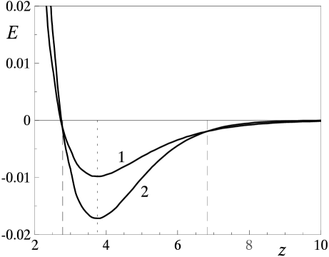
Figure 1: The ”interatomic” energy $E$, in units of $\alpha Z_{1}Z_{2}$, versus a dimensionless distance $z=\alpha R$. Curve 1 is appropriate to equation (108) and exhibits the case of a simple exponential charge clouds neutralizing central point charges of the distance $R$ apart. The case of the corresponding Gaussian charge clouds specified by formula (109) is described by curve 2, providing that its minimum coincides with the minimum point of curve 1 at $\mu=0.3586\alpha$ that is marked by the vertical dotted line. The dashed lines indicate the points of intersection of these curves.

not surprising because the next sample of this set, i.e. $W^{(3)}(R)$ described by (87), is specified by the same exponential decrease. Conversely, if the energy is determined by Gaussian spreading functions, then either of the contributions to (109) is specified by its own predominant law of decrease.

It seems to be interesting to recall that there is sometimes a tendency towards changing a simple exponential electron spreading by a Gaussian one in molecular calculations, where the contribution of the exchange interaction can then be evaluated in a much simpler manner [40, 41, 42, 43]. Although the direct Coulomb interaction is still the subject of our interest, this is the reason to compare results (108) and (109) in more amount of detail. To this end, we plot the corresponding energy curves together, as shown in figure 1. The shape of either of these curves is quite natural. Indeed, the energy is positive and its value tends to infinity as $R$ drops to zero. On the other hand, if $R$ grows, then the energy eventually becomes negative, attains at its minimum value and farther falls off

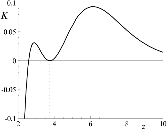
Figure 2: The parameter $K$ defined by formula (110) versus a dimensionless distance $z=\alpha R$. The position of energy minima, where $K$ has a local minimum, is pointed out by the vertical dotted line.

to zero in magnitude, being still negative. The latter is a direct consequence of the fact that just in general relation (107) the contribution of $W^{(2)}(R)$ as a function of $R$ is always more diffuse than that of $W^{(1)}(R)$. In order to compare both the curves, we have shifted a minimum point of the curve describing quantity (109) to the value of $R=3.745/\alpha$. We see that a minimum of curve 2 corresponding to $E_{\rm G}^{\rm{min}}=-0.01715\alpha Z_{1}Z_{2}$ is much deeper than that of curve 1 with the value of $E_{\rm s}^{\rm{min}}=-0.009805\alpha Z_{1}Z_{2}$ and this effect is described by the ratio 1.749. Moreover, the curvature of curve 2 at its minimum point is also greater than that of curve 1. As a result, there are two points of intersection between those curves which take place at $R=2.781/\alpha$ and at $R=6.830/\alpha$, with the energy values $E=-0.000652\alpha Z_{1}Z_{2}$ and $E=-0.00194\alpha Z_{1}Z_{2}$, respectively, as shown in figure 1 as well.

Of course, the energy $E_{\rm G}(z)$ can be further scaled by the factor $E_{\rm s}^{\rm{min}}/E_{\rm G}^{\rm{min}}$ so as to simulate the behaviour of $E_{\rm s}(z)$. The comparison of both these energies is then specified by the relative value of the form

$$K(z)=\Bigl{[}E_{\rm G}(z)\frac{E_{\rm s}^{\rm{min}}}{E_{\rm G}^{\rm{min}}}-E_{\rm s}(z)\Bigr{]}\frac{1}{|E_{\rm s}^{\rm{min}}|}=\frac{E_{\rm G}(z)}{|E_{\rm G}^{\rm{min}}|}-\frac{E_{\rm s}(z)}{|E_{\rm s}^{\rm{min}}|}.$$ (110)

The behaviour of $K(z)$ as a function of $z$ is shown in figure 2. We see that $K(z)$ turns out not to be monotonic in the vicinity of $z$ corresponding to minima of the energies at hand. This fact can be important upon minimizing a total energy modified by other energy contributions. In this case the effect driven by simple exponential spreading functions and that driven by Gaussian spreading functions are expected to be far from being proportional.

9 Conclusion

In summary, it is shown that the effect of charge spreading proposed by Bertaut [21, 27] can be utilized in a multiple manner. It means that the problem how many times a given spreading function is applied to the original charge distribution in a crystal is not of principle. Nevertheless, the tendency towards increasing the rate of convergence upon multiple charge spreading is just recognized by Bertaut [27] and will be confirmed elsewhere [32]. This result is not trivial. Presumably, it is associated with an idea that there is an optimum spreading configuration with very diffuse tails. In this connection, the fact that all the effects driven by a Gaussian spreading function are reproduced in the same functional form, regardless of its multiple application, may anyhow point to an optimum character of a Gaussian spreading.

Here we also recognize that a certain spreading, either single or multiple, may be attributed to every point of space and so may be treated as a uniform transformation of space. It is significant that the general relation between electrostatic potentials and specific Coulomb energies in crystals, as well as zero value of the mean potential there, turns out to be invariant with respect to such a transformation.

It is evident that the application of a multiple charge spreading to the problem of lattice summation is nothing but a fruitful approach to that problem. It implies that the final results of lattice summation are to be independent of the shape of spreading. However, it is not the case if the charge spreading is regarded as a real property of at least a pair of complex neutral physical objects connected by the Coulomb interaction. In this event the replacement of a natural shape of, for example, an electron cloud with a more artificial shape must be performed with caution.

Appendix A Some general relations for charge spreading

Equation (37) can be readily rewritten as

$${\mathit{\Omega}}^{(n)}(|{\bi{R}}|)=\int\sigma(|{\bi{r}}|){\mathit{\Omega}}^{(n-1)}(|{\bi{R}}+{\bi{r}}|)\,d{\bi{r}}.$$ (111)

With making use of spherical coordinates of ${\bi{r}}$, we assume that

$$|{\bi{R}}+{\bi{r}}|=\bigl{(}R^{2}+r^{2}+2Rr\cos\theta\bigr{)}^{1/2}\equiv y$$ (112)

and go over from the variable $\theta$ to a new variable $y$. The result of integration over $y$ is then of form (71). On the other hand, if ${\bi{R}}=0$, then the integration over angular variables of ${\bi{r}}$ in (111) is trivial and we obtain issue (72).

The case of ${\mathit{\Omega}}^{(1)}(R)$ is straightforward and is described by

$${\mathit{\Omega}}^{(1)}(R)=\frac{1}{R}-4\pi\int_{R}^{\infty}\sigma(r)\Bigl{(}\frac{r}{R}-1\Bigr{)}r\,dr.$$ (113)

Equations (73) and (74) follow therefrom. If we are interested in ${\mathit{\Omega}}^{(2)}(R)$, then the employment of (113) in the general relation (71) gives rise to

$${\mathit{\Omega}}^{(2)}(R)={\mathit{\Omega}}^{(1)}(R)-\frac{8\pi^{2}}{R}\int_{0}^{\infty}\sigma(r)J(R,r)r\,dr,$$ (114)

where we utilized definition (113) again and

$$J(R,r)=\int_{|R-r|}^{R+r}dy\int_{y}^{\infty}\sigma(r^{\prime})(r^{\prime}-y)r^{\prime}\,dr^{\prime}.$$ (115)

If we interchange the order of integration over $r^{\prime}$ and $y$ here, then the integration over $y$ is straightforward and we obtain

$$J(R,r)=\frac{1}{2}\int_{|R-r|}^{\infty}\sigma(r^{\prime})\bigl{(}|R-r|-r^{\prime}\bigr{)}^{2}r^{\prime}\,dr^{\prime}-\frac{1}{2}\int_{R+r}^{\infty}\sigma(r^{\prime})\bigl{(}R+r-r^{\prime}\bigr{)}^{2}r^{\prime}\,dr^{\prime}.$$ (116)

In turn, based on (23), it is expedient to rewrite expression (113) in an identical form

$${\mathit{\Omega}}^{(1)}(R)=\frac{1}{R}-\frac{16\pi^{2}}{R}\int_{0}^{\infty}\sigma(r)r\,dr\int_{R}^{\infty}\sigma(r^{\prime})r^{\prime}\bigl{[}r(r^{\prime}-R)\bigr{]}dr^{\prime}.$$ (117)

Substituting (116) and (117) into (114) and combining the integral terms, we arrive at the result in the most symmetric form given by formulae (75), (77) and (78), in agreement with (40). On the other hand, relation (76) for ${\mathit{\Omega}}^{(2)}(0)$ appears directly upon substituting (113) into (72).

Appendix B Coulomb interaction between Gaussian functions

Here we follow the treatment of Boys [40]. Let us consider two charge distributions

$$\sigma_{\alpha}(r)=\exp(-\alpha r^{2}),\quad\sigma_{\beta}(r)=\exp(-\beta r^{2}).$$ (118)

According to (37), they determine the values

$${\mathit{\Omega}}^{(1)}_{\beta}(R)=\int\frac{\sigma_{\beta}(r)\,d{\bi{r}}}{|{\bi{R}}+{\bi{r}}|},$$ (119)

$${\mathit{\Omega}}^{(2)}_{\alpha\beta}(R)=\int\sigma_{\alpha}(r){\mathit{\Omega}}^{(1)}_{\beta}(|{\bi{R}}+{\bi{r}}|)\,d{\bi{r}},$$ (120)

where $R=|{\bi{R}}|$ and $r=|{\bi{r}}|$.

The particular form of the distributions in (118) enables one to go over to the variable ${\bi{r}}^{\prime}={\bi{r}}+{\bi{R}}$ in equation (119). The integration over the angular coordinates of ${\bi{r}}^{\prime}$ is then trivial there and we obtain

$${\mathit{\Omega}}^{(1)}_{\beta}(R)=\frac{2\pi}{\beta R}\int_{0}^{R}\exp(-\beta x^{2})\,dx,$$ (121)

where $x=|{\bi{r}}^{\prime}|$. Inserting (121) into (120) and operating further in the same manner, we derive

$${\mathit{\Omega}}^{(2)}_{\alpha\beta}(R)=\frac{2\pi^{2}}{\alpha\beta R}I(R),$$ (122)

where

$$I(R)=\int_{-\infty}^{\infty}\exp[-\alpha(R-y)^{2}]\,dy\int_{0}^{y}\exp(\beta x^{2})\,dx.$$ (123)

If we differentiate equation (123) with respect to $R$, then we obtain

$$\frac{dI(R)}{dR}=-\int_{-\infty}^{\infty}\frac{d}{dy}\Bigl{\{}\exp[-\alpha(R-y)^{2}]\Bigr{\}}\,dy\int_{0}^{y}\exp(\beta x^{2})\,dx.$$ (124)

Integrating the right-hand side of (124) by parts, we easily reach

$$\frac{dI(R)}{dR}=\sqrt{\frac{\pi}{\alpha+\beta}}\exp\Bigl{(}-\frac{\alpha\beta}{\alpha+\beta}R^{2}\Bigr{)}.$$ (125)

Note that $I(0)=0$ follows from (123) and specifies the further integration of (125) with respect to $R$. On inserting the result of integration into equation (122), the final issue takes the form

$${\mathit{\Omega}}^{(2)}_{\alpha\beta}(R)=\frac{2\pi^{5/2}}{\alpha\beta\sqrt{\alpha+\beta}R}\int_{0}^{R}\exp\Bigl{(}-\frac{\alpha\beta z^{2}}{\alpha+\beta}\Bigr{)}\,dz$$ (126)

that is naturally symmetric with respect to $\alpha$ and $\beta$.

References

References

• [1] Tosi M P 1964 Solid State Physics ed F Seitz and D Turnbull volΒ 16 (New York: Academic Press) ppΒ 1–120;
• [2] Glasser M L and Zucker I J 1980 Theoretical Chemistry: Advances and Perspectives ed H Eyring and D Henderson volΒ 5 (New York: Academic Press) ppΒ 67–139
• [3] Kholopov E V 2004 Usp. Fiz. Nauk 174 1033 [Phys.–Usp. 47 965]
• [4] Wolf D, Keblinski P, Phillpot S R and Eggebrecht J 1999 J. Chem. Phys. 110 8254
• [5] Marshall S L 2000 J. Phys.: Condens. Matter 12 4575
• [6] Demontis P, Spanu S and Suffritti G B 2001 J. Chem. Phys. 114 7980
• [7] Marshall S L 2002 J. Phys.: Condens. Matter 14 3175
• [8] Venkatesh P K 2002 Physica B 318 121
• [9] Tyagi S 2004 Phys. Rev. E 70 066703
• [10] Pask J E and Sterne P A 2005 Phys. Rev. B 71 113101
• [11] Tyagi S 2005 J. Chem. Phys. 122 014101
• [12] Harrison W A 2006 Phys. Rev. B 73 212103
• [13] Ewald P P 1921 Ann. Phys. 64 253
• [14] Grzybowski A, GwΓ³ΕΊdΕΊ E and BrΓ³dka A 2000 Phys. Rev. B 61 6706
• [15] Porto M 2000 J. Phys. A: Math. Gen. 33 6211
• [16] Wheeler D R and Newman J 2002 Chem. Phys. Lett. 366 537
• [17] Zhang S and Chen N 2002 Phys. Rev. B 66 064106
• [18] Kholopov E V 2007 J. Phys. A: Math. Theor. 40 6101
• [19] Nijboer B R A and De Wette F W 1957 Physica 23 309
• [20] Sugiyama A 1984 J. Phys. Soc. Japan 53 1624
• [21] Bertaut F 1952 J. Phys. Radium 13 499
• [22] Luty B A, Tironi I G and van Gunsteren W F 1995 J. Chem. Phys. 103 3014
• [23] Templeton D H 1955 J. Chem. Phys. 23 1629
• [24] Jenkins H D B 1971 Chem. Phys. Lett. 9 473
• [25] Weenk J W and Harwig H A 1975 J. Phys. Chem. Solids 36 783
• [26] Herzig P 1981 Chem. Phys. Lett. 84 127
• [27] Bertaut E F 1978 J. Phys. Chem. Solids 39 97
• [28] Argyriou D N and Howard C J 1992 Aust. J. Phys. 45 239
• [29] Bethe H 1928 Ann. Phys. 87 55
• [30] Reining L and Del Sole R 1990 Phys. Stat. Sol. b 162 K37
• [31] Harris F E and Monkhorst H J 1970 Phys. Rev. B 2 4400
• [32] Kholopov E V 2008 to be published
• [33] Kholopov E V 2006 Phys. Stat. Sol. b 243 1165
• [34] Kanamori J, Moriya T, Motizuki K and Nagamiya T 1955 J. Phys. Soc. Japan 10 93
• [35] Jones R E and Templeton D H 1956 J. Chem. Phys. 25 1062
• [36] Herzig P 1979 Chem. Phys. Lett. 68 207
• [37] Heyes D M 1981 J. Chem. Phys. 74 1924
• [38] Birman J L 1958 J. Phys. Chem. Solids 6 65
• [39] Whittaker E T and Watson G N 1927 A Course of Modern Analysis (Cambridge: Cambridge Univ. Press) p 114
• [40] Boys S F 1950 Proc. R. Soc. London A 200 542
• [41] McWeeny R 1953 Acta Crystallogr. 6 631
• [42] Lombardi E and Jansen L 1966 Phys. Rev. 151 694
• [43] de Castro E V R and Jorge F E 1998 J. Chem. Phys. 108 5225