Using dynamically scattered electrons for 3-dimensional potential reconstruction

Abstract

Three-dimensional charge density maps computed by first-principles methods provide information about atom positions and the bonds between them, data which is particularly valuable when trying to understand the properties of point defects, dislocations, and interfaces. This letter presents a method by which 3-dimensional maps of the electrostatic potential, related to the charge density map by the Poisson equation, can be obtained experimentally at 1 Å  resolution or better. This method requires data acquired by holographic transmission electron microscopy (TEM) methods such as off-axis electron holography or focal series reconstruction for different directions of the incident electron beam. The reconstruction of the 3-dimensional electrostatic (and absorptive) potential is achieved by making use of changes in the dynamical scattering within the sample as the direction of the incident beam varies.

Extended defects such as dislocations, interfaces, in particular solid liquid interfaces, pose a particular challenge to atomic scale computational methods. While their complexity normally requires super-cells too large for ab-initio methods, the long-range nature of forces determining their properties (e.g. strain fields, Coulomb and van der Waals [dispersion] forces) makes the construction of reliable yet efficient interatomic potentials required for molecular dynamics (MD) and related computational methods an extremely complicated task. Being able to perform experiments which directly map the 3-dimensional local electrostatic potential would provide a wealth of information without the need to do any simulations at all and, if computations are needed to extract information not provided by the potential map or, in the case of MD, it would allow verification of interatomic potentials by direct comparison between experiment and simulation for the very (defect) structure under investigation. For single crystals of small unit cell it has recently been demonstrated that it is possible to map the bond charge distribution by fitting Fourier coefficients of the crystal potential to convergent beam electron diffraction (CBED) data Zuo99 .

TEM images, in the context of focal series reconstruction (inline holography) over a large defocus range Koch08FRWR , are very sensitive to relative atomic positions and variations in the electrostatic potential. Although claiming to be able to provide data on the 3-dimensional distribution of atoms this is not true for destructive methods such as 3D atom probe Blavette93 because the atoms being ”imaged” are not extracted from their original environment, but from the sample surface.

The enormous advantages of TEM imaging come at the price of the lack of a general direct interpretability at atomic resolution. Although modern electron optics has been able to remove many of the artefacts caused by aberrations of the imaging system, it cannot remove artefacts produced by the multiple (or dynamical) scattering process itself. This is the main reason why electron tomography has never been applied at atomic resolution, with the exception of extremely small nanostructures consisting of light atoms, for which the authors felt that they could neglect dynamical electron scattering events BarSadan08 . Attempts to correct for artefacts (i.e. features which cannot be interpreted directly in terms of atomic structure) in the exit face wave function produced by dynamical scattering effects have, in the case of thin or non-crystalline samples, at most been able to reconstruct an average projected potential Gribulek91 ; Beeching93 ; Scheerschmidt98 ; Lentzen00 ; Allen01_dyn .

The method presented in this letter directly reconstructs the local complex scattering potential on a 3-dimensional grid, the real part of which is the electrostatic potential, by separating the multiple scattering paths between potential voxels.

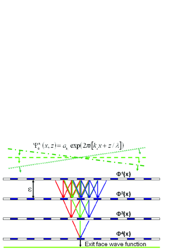
Figure 1: (color online) Diagram of real-space multislice algorithm. The scattering of the incident electron beam described by a plane wave is approximated by a finite number of scattering events at equidistant layers partitioning the sample in $z$-direction. As a consequence, the signal in the exit face wave function is non-local, including contributions from a number of scattering paths, the relative phase of which can be varied by changing the illumination tilt angle $\theta_{x}=\sin^{-1}k_{x}\lambda$.

The following discussion will, in order to keep the equations readable, only consider the reconstruction of a 2-dimensional structure from a series of 1-dimensional images. The extension to 3 dimensions is straight forward, requiring only small changes in the presented formalism.

The proposed reconstruction method is based on the real-space variant vanDyck80 of the multislice algorithm Cowley57 for solving the relativistically corrected Schrödinger equation describing the propagation of a fast electron through the specimen potential (see figure 1 for an illustration). In a first step the 2-dimensional scattering potential (remember that this discussion can easily be extended to 3 dimensions) is divided into a set of $N$ discrete horizontal slices of thickness $\epsilon$ (the optical axis of the microscope is assumed to be vertical, the fast beam electrons travelling down the microscope column) and the potential within a slice of index $m$ is projected into a 1-dimensional layer of potential

$$V^{(m)}(x)=\int_{\epsilon(m-1/2)}^{\epsilon(m+1/2)}V(x,z)dz.$$

The electron propagation is then approximated by multiplication of the incident wave function by a phase grating $\Phi^{(m)}(x)=\exp[i\sigma V^{(m)}(x)])$ ($\sigma=2\pi\left(m_{e}c^{2}+E_{0}\right)/\left[\lambda E_{0}\left(2m_{e}c^{2}+E_{0}\right)\right]$ being the electron-potential interaction constant) at the position of each slice and Fresnel propagation between the slices. We will assume an incident plane wave $A\exp(2\pi i\vec{k}\cdot\vec{r})=A\exp[2\pi i(k_{x}x+k_{z}z)]$ arriving at the sample at an angle $\theta=\sin^{-1}(k_{x}/k_{z})$. Since holographic experiments can measure relative phases but not the absolute phase of an electron wave functions we will define $z=0$ in the plane of the exit face wave function, fixing the z-dependence of the wave function at the entrance surface. Combining this z-dependent phase factor with the scaling factor $A$ we obtain $\Psi^{(k_{x})}(x)=A^{(k_{x})}\exp[2\pi ik_{x}x]$ at the entrance surface of the specimen. The electron wave function at the exit surface can then be obtained by the real-space multislice formalism vanDyck80 as

$$\Psi^{(k_{x})}(x) = \Phi^{(N)}(x)\cdot e^{\epsilon\lambda\left(\frac{i\Delta_{x}}{4\pi}-k_{x}\nabla_{x}\right)}\cdots$$ (1)

$$\cdot\Phi^{(2)}(x)\cdot e^{\epsilon\lambda\left(\frac{i\Delta_{x}}{4\pi}-k_{x}\nabla_{x}\right)}\Phi^{(1)}(x)$$

$$\cdot A^{(k_{x})}\exp[2\pi ik_{x}x]$$

Here $\lambda=1/k_{z}=hc/\sqrt{E_{0}\left(2m_{e}+E_{0}\right)}$ is the electron wavelength, $E_{0}$ the accelerating voltage, $h$ Planck’s constant, $c$ the speed of light, $m_{e}$ the mass of an electron, $\Delta_{x}$ the Laplace operator and $\nabla_{x}$ the gradient in the $x$-direction.

Implementing the multislice algorithm on a computer requires a discrete grid in the lateral dimension in addition to the discrete slices in the $z$-direction. Keeping the lateral sampling distance $\delta_{x}$ constant we may simplify the notation by defining a dimensionless imaginary parameter $\gamma_{k_{x}}=2\pi i\delta_{x}k_{x}$ and replacing $x$ by $j_{x}\delta_{x}$, $\Psi(x)$ by $\Psi_{j_{x}}$, $V^{(m)}(x)$ by $V^{(m)}_{j_{x}}$, $\Phi^{(m)}(x)$ by $\Phi^{(m)}_{j_{x}}$, and $\exp[2\pi ik_{x}x]$ by $\exp[\gamma_{k_{x}}j_{x}]$. This makes also the translation of the following equations into a computer program a bit more apparent.

Expanding the Fresnel propagation operator by using the relations

$$\Delta_{x}\Psi(x) = \frac{\Psi(x+\delta_{x})-2\Psi(x)+\Psi(x-\delta_{x})}{\delta_{x}^{2}}\quad\textrm{ and}$$

$$\nabla_{x}\Psi(x) = \frac{\Psi(x+\delta_{x})-\Psi(x-\delta_{x})}{2\delta_{x}}$$

we obtain

$$\exp\left[\frac{i\epsilon\lambda}{4\pi}\left(\Delta_{x}+\gamma_{k_{x}}\nabla_{x}\right)\right]\Psi(x)$$

$$= \left\{1+\frac{i\epsilon\lambda}{4\pi}\left(\Delta_{x}+\gamma_{k_{x}}\nabla_{x}\right)\right.$$

$$+\left.\frac{1}{2}\left[\frac{i\epsilon\lambda}{4\pi}\left(\Delta_{x}+\gamma_{k_{x}}\nabla_{x}\right)\right]^{2}+\ldots\right\}\Psi(x)$$

$$= \Psi(x)+\beta\left[(1+\gamma_{k_{x}})\Psi_{j_{x}+1}-2\Psi_{j_{x}}+(1-\gamma_{k_{x}})\Psi_{j_{x}-1}\right]$$

$$+\frac{\beta^{2}}{2}\left[(1+\gamma_{k_{x}})^{2}\Psi_{j_{x}+2}-4(1+\gamma_{k_{x}})\Psi_{j_{x}+1}\right.$$

$$\left.+(6-2\gamma_{k_{x}}^{2})\Psi_{j_{x}}-4(1-\gamma_{k_{x}})\Psi_{j_{x}-1}\right.$$

$$\left.+(1-\gamma_{k_{x}})^{2}\Psi_{j_{x}-2}\right]+O\left(\beta^{3}\right)$$ (2)

in orders of approximation of the Ewald sphere curvature given by the parameter $\beta=i\epsilon\lambda/\left(4\pi\delta_{x}^{2}\right)$. The sampling distance $\delta_{x}$ is typically quite a bit smaller than the image resolution defined by aberrations of the electron optics, the stability of the microscope, and the size of the objective aperture (e.g. $0.1\ldots 0.5$Å  for HRTEM at 1 Å  resolution).

By chosing the appropriate real-space sampling, slice thickness and electron accelerating voltage one can force $\beta$ to have a fairly small value. Plugging the expansion of the Fresnel propagator (2) into (1) we can expand the expression for the exit face wave function in orders of $\beta$. The first order expansion neglecting, for the moment, terms of order $\beta^{2}$ and higher looks as follows:

$$\Psi^{(k_{x})}_{j_{x}} = A^{(k_{x})}e^{\gamma_{k_{x}}j_{x}}\Phi^{(N)}_{j_{x}}\left\{\prod_{m=1}^{N-1}\Phi^{(m)}_{j_{x}}\right.$$ (3)

$$\left.+\beta\left[e^{\gamma_{k_{x}}}(1+\gamma_{k_{x}})\sum_{k=1}^{N-1}\prod_{m=1}^{k}\Phi^{(m)}_{j_{x}+1}\prod_{m=k+1}^{N-1}\Phi^{(m)}_{j_{x}}\right.\right.$$

$$\left.\left.+e^{-\gamma_{k_{x}}}(1-\gamma_{k_{x}})\sum_{k=1}^{N-1}\prod_{m=1}^{k}\Phi^{(m)}_{j_{x}-1}\prod_{m=k+1}^{N-1}\Phi^{(m)}_{j_{x}}\right.\right.$$

$$\left.\left.-2(N-1)\prod_{m=1}^{N-1}\Phi^{(m)}_{j_{x}}\right]+O(\beta^{2})\right\}$$

Note here, that the first term, the zeroth order expansion is independent of $\beta$ and is just the well-known phase object approximation which includes multiple scattering to $N^{th}$ order but neglects effects due to curvature and tilt of the Ewald sphere.

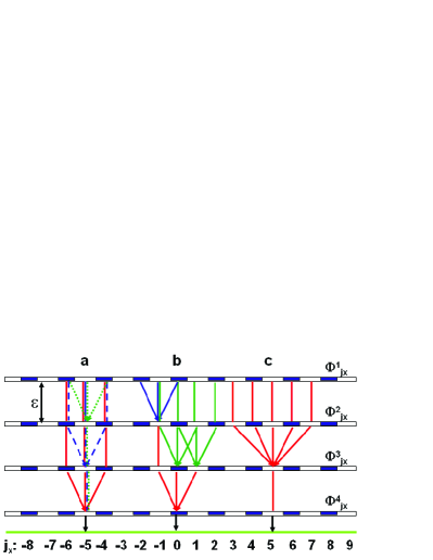
Figure 2: (color online) Diagram of first (A) and second order (B,C) approximation of the Ewald sphere curvature effects in the real-space multislice algorithm for $k_{x}=0$. The $\Delta_{x}$ operator is depicted by a node merging 3 paths, and the $\Delta_{x}^{2}$ operator by a node merging 5 paths. Multiplying the scattering potential along the the read solid, blue dashed and green dotted paths in A will produce all the possible monomials that are linear in $\beta$, i.e. which involve only a single $\Delta_{x}$ operator. Monomials resulting from paths shown in B and C (only one possible path is shown in each) are proportional to $\beta^{2}$ and involve either 2 successive $\Delta_{x}$ operations, or a single $\Delta_{x}^{2}$ operation.

Figure 2a illustrates expression (3) graphically for an object partitioned into 4 layers. Examples of the 2 possible scattering paths that scale as $\beta^{2}$ are shown in figure 2b and 2c. While the conventional multislice algorithm Ishizuka77 iterating between real and reciprocal space naturally includes all orders $\beta^{n}$, in real-space algorithms they need to be included explicitly. Since increasing $n$ slows down the computation enormously, terms $O(\beta^{n\geq 3})$ in the computation of a single Fresnel propagation are usually neglected. An algorithm approximating the Fresnel propagation up to $O(\beta^{n=1})$ will only have contributions of $O(\beta^{n\geq 2})$ to the final wave function of the type shown in figure 2b, i.e. multiple $\Delta_{x}$ operations, but neglect the equally important contributions shown in figure 2c.

The aim of this letter being the determination of the 3-dimensional scattering potential from the observed images we must consider the contributions to the exit face wave function in the order of significance, i.e. all terms up to a given order $O(\beta^{n})$. Taking a closer look at figure 2 makes clear that in order to reconstruct $N$ slices one needs to expand the Fresnel propagation up to at least $n=(N-1)/2$ (rounding up for even $N$). The resulting system of polynomial equations of degree $N$ is sparse and may be solved using globally convergent algorithms for solving multivariate polynomial sets of equations (see e.g. Sherali92 with an example application given in Koch08_LACBED ).

Holographic methods such as off-axis electron holography Moellenstedt56 , but also focal series reconstruction (see, for a very recent example, Koch08FRWR and references to 9 alternative algorithms therein) are able to reconstruct the complex exit face wave function for each incident beam tilt. If, as is common practice, in the off-axis holographic reconstruction the side band is properly centered, and in the focal series reconstruction the images are aligned by cross-correlation or similar methods, neither of these methods will reconstruct the global phase shift $\exp[\gamma_{k_{x}}j_{x}]$ that is associated with the tilted illumination (the relative phase factors in the second and third term of (3) remain, though). We can therefore drop this term alltogether. However, a reference point common to wave functions of different incident beam tilt must still be chosen in order to fix the complex coeffcients $A^{(k_{x})}$. A vacuum region or another area of well-known scattering properties within the field of view would be ideal, but if no such reference point can be defined the $A^{(k_{x})}$ parameters can also be included in the non-linear reconstruction algorithm. We will assume $A^{(k_{x})}=1$ in the example presented below.

For demonstration purposes, and in order to reveal the principles of the proposed methodology independent of the performance of a given polynomial equation solver we approximate the system of polynomial equations (3) by expanding the phase grating $\Phi^{(m)}_{j_{x}}$ in terms of the potential assuming the validity of the weak phase object approximation. For a structure that has been split into $N=3$ layers we approximate

$$\Phi^{(3)}_{j_{x3}}\Phi^{(2)}_{j_{x2}}\Phi^{(1)}_{j_{x1}} = e^{i\sigma V^{(3)}_{j_{x3}}}e^{i\sigma V^{(2)}_{j_{x2}}}e^{i\sigma V^{(1)}_{j_{x1}}}$$

$$\approx 1+i\sigma V^{(3)}_{j_{x3}}+i\sigma V^{(2)}_{j_{x2}}+i\sigma V^{(1)}_{j_{x1}}$$

converting (3) into a linear system of equations, the solution of which should be straight forward. It turns out the the matrix defining the resulting system of equations is slightly rank-deficient, because dropping all the non-linear terms in $V^{(m)}_{j_{x}}$ introduces 2 additional degrees of freedom, the overall phase relationship between the 3 layers. Defining the relative potential of 1 column of pixels (e.g. in the example shown in figure 3 I defined 3 additonal linear equation that force the potential to be zero (vacuum) for the right most pixel in each of the 3 layers) will remove this degree of freedom and produce, in the absence of noise, a unique reconstruction. The system of linear equations has been solved using singular value decomposition.

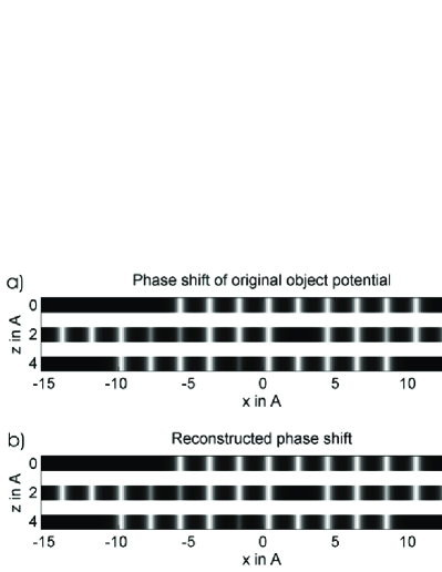
Figure 3: Phase shift $\phi^{(m)}(x)=\sigma V^{(m)}(x)$ for a 3-layered ”phantom” structure (a) and the phase shift reconstructed from it using the linear approximation to (3) (b) demonstrating a 3-dimensional reconstruction at atomic resolution. The scattering factor and lattice constant correspond to that of gold. The ”defect” sites have been created by simply scaling the scattering factor of gold by a number less than 1 (individual defects from left to right: second row: 0.5, 0.5, 0, 0.7, third row: 0.3). Apsorption has been included by multiplying the potential $V^{(m)}(x)$ by $(1+0.1i)$. Simulation parameters: object potential grid: $240\times 3$ pixels, $\delta_{x}=0.128$Å, $\epsilon=2.04$Å, $E_{0}=60$kV, $\sigma=0.0011$ (VÅ)^-1, $\beta=0.49i$, 5 different tilt angles of the incident beam: $\theta=-1^{\circ}$ ($\gamma_{k_{x}}=-0.29i$), $\theta=-0.3^{\circ}$ ($\gamma_{k_{x}}=-0.086i$), $\theta=0^{\circ}$ ($\gamma_{k_{x}}=0i$), $\theta=0.7^{\circ}$ ($\gamma_{k_{x}}=0.20i$), $\theta=1^{\circ}$ ($\gamma_{k_{x}}=0.29i$).

Figure 3 a shows the phase shift of a trial structure that has been sliced into 3 equidistant slices. Scattering factors and length scales have been scaled to those of the gold (110) lattice, in order to mimic actual experimental conditions. Since no noise has been included in this test, it is not surprising that reconstruction and original look identical. The fairly low accelerating voltage of only 60kV causes $\sigma$ (multiple scattering strength), $\beta$ (Ewald sphere curvature) and $\beta\gamma_{k_{x}}$ (illumination tilt sensitivity) to be of large enough values to make a 3-dimensional atomic resolution reconstruction of nano structures feasible, even in the presence of noise and for small beam tilt angles.

Some iterative tomographic reconstruction algorithms allow the specimen geometry to be used as a constraint, in principle being able to reconstruct an object consisting of only $N$ distinct layers to be reconstructed from $N$ projections only. The angle between these $N$ projections must, however, be quite large. Although requiring the same minimum number of tilt angles, in contrast to (linear) tomography, where the 3-dimensional information is introduced by projecting along different directions, making use of dynamical scattering as proposed here, implies a tilt-angle dependent (complex) weighting factor for a set of monomials in the polynomial system of equations (3). These weighting factors depend strongly on the accelerating voltage and can therefore be tuned to the scattering strength of the material, available beam tilt range and desired resolution in the direction parallel to the electron beam. Modern TEMs being able to achieve atomic resolution imaging at $E_{0}\leq 60kV$ (e.g. Kisielowski08 ) will therefore be able to image the 3-dimensional potential distribution within nanostructures at atomic resolution without having to tilt the specimen.

It should be noted that exit wave reconstruction for several illumination tilt angles is only one of several methods for acquiring the experimental data required for the 3D reconstruction described above. Alternative methods include Rönchigram focal series recorded for different illumination or specimen shifts and, of course, holographic experiments at different specimen tilts.

Summarizing, a method for reconstructing the 3-dimensional electrostatic potential of a TEM sample has been proposed. The method is based on a reformulation of the real-space multislice formalism for computing the multiple scattering of a fast electron within a TEM sample in terms of a polynomial set of equations, identifying and keeping the most significant terms. The solution of the resulting sparse multivariate polynomial system of equations can be found by applying polynomial equation global optimization algorithms available in the literature.

In the special case that the weak phase object approximation is valid the polynomial system of equation transforms into a linear system of equations which can be solved by standard methods. Applying this simplification a 2-dimensional complex test object consisting of 3 layers has been reconstructed successfuly from 5 1-dimensional electron wave functions simulated for illumination tilt angles ranging from $-1^{\circ}$ to $+1^{\circ}$. The construction of an efficient global optimization algorithm specialized for the particular type of systems of polynomial equations described in this letter is planned for the near future.

- (1) J.M. Zuo, M. Kim, M. O’ Keeffe, J.C.H. Spence, Nature 401, 49 (1999)
- (2) D. Blavette, B. Deconihout, A. Bostel, J.M. Sarrau, M. Bouet, A. Menand, Rev. Sc. Instr. 64, 2911 (1993)
- (3) M. Bar Sadan, Nano Letters 8, 891 (2008)
- (4) M.A. Gribelyuk, Acta Cryst. A47, 715 (1991)
- (5) M.J. Beeching and A.E.C. Spargo, Ultramicroscopy 52, 243 (1993) 243.
- (6) K. Scheerschmidt, J. Microscopy 190, 238 (1998) 243.
- (7) M. Lentzen and K. Urban, Acta Cryst. A56, 235 (2000)
- (8) L.J. Allen, C.T. Koch, M.P. Oxley, and J.C.H. Spence, Acta Cryst. A57, 473 (2001)
- (9) D. van Dyck, J. Microscopy 119, 114 (1980)
- (10) J.M. Cowley and A.F. Moodie, Acta Cryst. 10, 609 (1957)
- (11) G. Möllenstedt and H. Düker, Z. Phys. 145, 377, (1956)
- (12) C.T. Koch, Ultramicroscopy 108, 141 (2008)
- (13) K. Ishizuka and N. Uyeda, Acta Cryst. A33, 740 (1977)
- (14) H. D. Sherali and C. H. Tuncbilek, Journal of Global Optimization 2, 101-112 (1992)
- (15) C. T. Koch, Phys. Pev. Lett. submitted (2008)
- (16) C. Kisielowski et al., Microscopy and Microanalysis 14, 469 (2008)