Anderson localization in a correlated fermionic mixture

Anderson localization in correlated fermionic mixtures

Abstract

A mixture of two fermionic species with different masses is studied in an optical lattice. The heavy fermions are subject only to thermal fluctuations, the light fermions also to quantum fluctuations. We derive the Ising-like distribution for the heavy atoms and study the localization properties of the light fermions numerically by a transfer-matrix method. In a two-dimensional system one-parameter scaling of the localization length is found with a transition from delocalized states at low temperatures to localized states at high temperature. The critical exponent of the localization length is $\nu\approx 0.88$.

The question of Anderson localization in an ultra cold gas has attracted considerable attention recently by a number of experimental groups ospelkaus06 ; roati08 ; billy08 . Although the phenomenon itself has been studied in great detail over the last 50 years by many theoretical groups for various physical systems anderson58 ; abraham79 ; wegner76 , its experimental observation has been difficult. One of the reasons is that Anderson localization is an interference effect of waves due to elastic scattering in a random environment (disorder). Real systems, however, experience also substantial inelastic scattering (e.g. absorption of electromagnetic waves by the scattering atoms, Coulomb interaction in electronic systems etc.) This may hamper the direct observation of Anderson localization significantly. Another reason is that random scattering is difficult to control in a real system. This is important in order to distinguish Anderson localization from simple trapping due to local potentials. It requires some kind of averaging over an ensemble of randomly distributed scatterers.

Ultra cold gases offer conditions, where most physical parameters are controllable. Since the atoms are neutral, there is no Coulomb interaction, and at sufficiently high dilution the interatomic collisions are negligible. Moreover, a periodic potential (optical lattice) can be applied by counterpropagating laser fields. This enables us to control the kinetic properties of the gas atoms by creating a specifically designed dispersion. Disorder could be created by disturbing the periodicity of the optical lattice. In practice, however, this is not easy because real disorder would require infinitely many laser frequencies. A first attempt is to study the superposition of two laser fields with “incommensurate” frequencies (i.e. the ratio of the two frequencies is an irrational number) roati08 . An alternative is to randomize the laser field by sending it through a diffusing plate billy08 .

Recent progress in atomic mixtures stan04 has offered another possibility to create disorder in an atomic system. Mixing of two different atomic species, where one is heavier than the other, creates a situation where the light atoms are scattered by the randomly distributed heavy atoms gavish05 ; ates05 ; maska08 ; ziegler08 . An optical lattice is applied in order to keep the heavy atoms in quenched positions. Due to their higher mass, the heavy atoms behave classically in contrast to the light atoms, which can tunnel in the optical lattice. A crucial question is what determines the distribution of the heavy atoms. The most direct distribution is obtained by putting atoms randomly in the optical lattice “by hand”, each of them with independent probability gavish05 . This case corresponds to uncorrelated disorder. Another possibility is to fill the optical lattice with both atomic species and consider a repulsive (local) interaction between them. Then the two species have to arrange each other such that the total atomic system presents a grand-canonical ensemble at a given temperature and a given lattice filling. In the presence of interparticle interaction within each atomic species there is a complex interplay of interaction and localization effect. This makes it difficult to isolate the effect of Anderson localization. In order to avoid interaction within each species we choose spin-polarized fermions in an optical lattice. Then only the Pauli principle controls the short-range interaction within each species, such that the remaining interaction is between the different fermionic species. It has been shown that then the light atoms are subject to a quenched average with respect to a thermal distribution of the heavy atoms, and that the distribution is related to an Ising-like model ates05 ; ziegler06 ; maska08 . The latter implies (strong) correlations between the heavy atoms. For systems in more than one dimension there is a critical temperature $T_{c}$ at which the correlation length diverges. This system provides several interesting features for studying Anderson localization. Although it is a many-body system, the light atoms behave effectively like independent (spinless fermionic) quantum particles in a random potential. The correlation of the randomness can be controlled by temperature, where the correlation length decreases with increasing temperature for temperatures $T>T_{c}$, or by the strength of the inter-species scattering.

In the following we shall study diffusion and Anderson localization in the grand-canonical ensemble of two spin-polarized fermionic species in one and two dimensions. Motivated by recent experimental study on a dilute BEC in $d=1$ billy08 , we consider a realistic scenario, in which an initial state is prepared at the center with a trapping potential and then it is released by opening (i.e. switching off) the trap. The expansion of the wave function is observed within our numerical procedure.

model: $c^{\dagger}$ ($c$) are creation (annihilation) operators of the light fermionic atoms, $f^{\dagger}$ ($f$) are the corresponding operators of the heavy fermionic atoms. This gives the formal mapping ${}^{6}{\rm Li}\rightarrow c^{\dagger}_{r},c_{r}$ and ${}^{40}{\rm K}\ (^{23}{\rm Na},\ ^{87}{\rm Rb})\rightarrow f^{\dagger}_{r},f_{r}$. The physics of the mixture of atoms is defined by the asymmetric Hubbard Hamiltonian

$$H=-{\bar{t}}_{c}\sum_{\langle r,r^{\prime}\rangle}c_{r}^{\dagger}c_{r^{\prime}}-{\bar{t}}_{f}\sum_{\langle r,r^{\prime}\rangle}f_{r}^{\dagger}f_{r^{\prime}}$$

$$-\sum_{r}\Big{[}\mu_{c}c_{r}^{\dagger}c_{r}+\mu_{f}f_{r}^{\dagger}f_{r}-Uf^{\dagger}_{r}f_{r}c^{\dagger}_{r}c_{r}\Big{]}.$$ (1)

The effective interaction within each species is controlled by the (repulsive) Pauli principle, whereas the interaction strength of different atoms is $U$. If the $f$ atoms are heavy, the related tunneling rate is very small. The limit ${\bar{t}}_{f}=0$ is known as the Falicov-Kimball model falicov69 ; farkasovsky97 ; freericks03 ; maska08 .

A grand-canonical ensemble of fermions at the inverse temperature $\beta=1/k_{B}T$ is defined by the partition function

$$Z={\rm Tr}e^{-\beta H}.$$

In the FK limit ${\bar{t}}_{f}=0$ the Hamiltonian of the light atoms $H_{c}(\{n_{r}\})$ depends only on the real numbers $\{n_{r}\}$ ($n_{r}=0,1$), and it is a quadratic form with respect to the $c$ operators of the light atoms:

$$\sum_{r,r^{\prime}}h_{c;rr^{\prime}}c^{\dagger}_{r}c_{r^{\prime}}=-{\bar{t}}_{c}\sum_{\langle r,r^{\prime}\rangle}c_{r}^{\dagger}c_{r^{\prime}}+\sum_{r}(Un_{r}-\mu_{c})c^{\dagger}_{r}c_{r}\ .$$ (2)

This means that the density fluctuations $n_{r}=f_{r}^{\dagger}f_{r}$ have been replaced by classical variables $n_{r}=0,1$. Thus $H_{c}(\{n_{r}\})$ describes non-interacting fermions which are scattered by heavy atoms, represented by $n_{r}$. The trace ${\rm Tr}_{c}$ in the partition function can be evaluated and gives a fermion determinant:

$$Z=\sum_{\{n_{r}\}}e^{\beta\mu_{f}\sum_{r}n_{r}}{\rm Tr}_{c}\left(e^{-\beta H_{c}(\{n_{r}\})}\right)$$

$$=\sum_{\{n_{r}\}}e^{\beta\mu_{f}\sum_{r}n_{r}}{\rm det}[{\bf 1}+e^{-\beta h_{c}}]\ .$$ (3)

The right-hand side is a sum over (non-negative) statistical weights. After normalization we can define

$$P(\{n_{r}\})={1\over Z}e^{\beta\mu_{f}\sum_{r}n_{r}}{\rm det}[{\bf 1}+e^{-\beta h_{c}}]$$ (4)

which gives $\sum_{\{n_{r}\}}P(\{n_{r}\})=1$. Thus $P(\{n_{r}\})$ is a probability distribution for correlated disorder and describes the distribution of the heavy atoms. In the strong-coupling regime ${\bar{t}}_{c}^{2}/2U\gg 1$ the distribution becomes an Ising model with nearest-neighbor coupling. At half-filling (i.e. $\mu_{f}=\mu_{c}=U/2$) this reads ates05

$$P(\{S_{r}\})\propto\exp\left(-\beta({\bar{t}}_{c}^{2}/2U)\sum_{<r,r^{\prime}>}S_{r}S_{r^{\prime}}\right)$$ (5)

where $S_{r}=2n_{r}-1$.

$\begin{array}[]{cc}\includegraphics[width=113.81102pt]{Chmulti.eps}&\includegraphics[width=113.81102pt]{Isingmulti.eps}\end{array}$

Figure 1: Real time evolution of a wave packet. At low temperature ($T=0$: left panel) it propagates due to the checker-board configuration of the heavy atoms. At larger temperature ($T=0.2$: right panel), the wave packet is localized due to a disordered configuration of heavy atoms.

localization: A trapped atomic cloud may be in the state $|i\rangle$, concentrated at the center of the optical lattice. After switching off the trapping potential the dynamics of the atomic cloud is described by the evolution equation $|\Psi_{t}\rangle=e^{-iHt}|i\rangle$. The optical lattice remains present during the evolution of the cloud. The expansion of the cloud of light atoms is studied numerically. Depending on the temperature of the grand-canonical system, we find a spreading of the wave function at low temperatures but a localized behavior at high temperatures (cf. Fig. 1). Apparently, there is a critical regime with some critical temperature $T_{c}^{\prime}$, which separates the spreading behavior from the localized behavior.

The local density of particles at site $r$ of the optical lattice with respect to the state $|\Psi_{t}\rangle$ reads

$$N_{r}=\langle\Psi_{t}|c^{\dagger}_{r}c_{r}|\Psi_{t}\rangle=\langle i|e^{iHt}c^{\dagger}_{r}c_{r}e^{-iHt}|i\rangle$$

with the initial state $|i\rangle=c^{\dagger}_{0}|0\rangle$. The state $|0\rangle$ is an equilibrium state of the entire system and can be expanded in terms of energy eigenfunctions and Boltzmann weights at the inverse temperature $\beta$:

$$\langle N_{r}\rangle={\sum_{k}e^{-\beta E_{k}}\langle E_{k}|c_{0}e^{iHt}c^{\dagger}_{r}c_{r}e^{-iHt}c^{\dagger}_{0}|E_{k}\rangle\over\sum_{k}e^{-\beta E_{k}}}$$

$$={1\over Z}{\rm Tr}\left[e^{-\beta H}c_{0}e^{iHt}c^{\dagger}_{r}c_{r}e^{-iHt}c^{\dagger}_{0}\right].$$ (6)

For the FK model this expression can also be written as a quenched average with respect to the distribution of heavy particles ziegler06 :

$$\langle N_{r}\rangle=\langle{\cal G}_{0r}^{\dagger}(t){\cal G}_{r0}(t)\rangle_{f}$$ (7)

with the single-particle Green’s function

$${\cal G}_{rr^{\prime}}(t)=[e^{-ith_{c}}({\bf 1}+e^{-\beta h_{c}})^{-1}]_{rr^{\prime}}\ .$$

$\langle...\rangle_{f}$ is the average with respect to the statistical weight of Eq. (4) or Eq. (5). For a given configuration $\{n_{r}\}$ of heavy atoms the Green’s function can also be expressed by eigenfunctions of the single-particle Hamiltonian $h_{c}$ in Eq. (2) ($h_{c}\phi_{k}=e_{k}\phi_{k}$). The spatial properties of these eigenfunctions determine the spreading of the average density particle density $\langle N_{r}\rangle$ through the Green’s function:

$${\cal G}_{r0}(t)=\sum_{k}e^{-ie_{k}t}\frac{\phi_{k,r}^{*}\phi_{k,0}}{1+e^{-\beta e_{k}}}\ .$$ (8)

The denominator represents the Fermi function, since our atoms are fermions. According to the localization theory, it can be assumed that $|\phi_{k,r}|\sim e^{-|r|/\xi_{k}}$, where $\xi_{k}$ is the localization length.

After a Fourier transformation of the time-dependent density in Eq. (7), the $\omega=0$ Fourier component of $\langle N_{r}\rangle$ reads

$${\bar{N}}_{r}=\sum_{k}\frac{|\phi_{k,r}^{*}\phi_{k,0}|^{2}}{(1+e^{-\beta e_{k}})^{2}}\sim\frac{e^{-2|r|/\xi}}{(1+e^{-\beta e_{k_{0}}})^{2}}\ \ \ (r\sim\infty)\ ,$$

where $\xi$ is the largest localization length and $e_{k_{0}}$ the corresponding energy level. Thus the expansion of the wave packet on large scales is controlled by $\xi$.

The localization length can be studied under the change of length scales by considering a finite optical lattice of length $L$ and width $M$ abraham79 . In particular, we analyze the change of the localization length with respect to the width $M$. For this purpose, we define the reduced (or normalized) localization length as $\Lambda_{M}=\xi/M$ and calculate this quantity by means of a numerical transfer-matrix approach mackinnon83 . $\Lambda_{M}$ either increases (delocalized states) or decreases (localized states) with the width $M$, depending on the system parameters (e.g. the inverse temperature $\beta$). There can also be a marginal behavior (e.g. for a special value $\beta_{c}^{\prime}$), where $\Lambda_{M}$ does not change with $M$. The latter indicates the existence of a phase transition from localized to delocalized states. A quantitative description of the behavior near $\beta_{c}^{\prime}$ can be based on the one parameter scaling hypothesis abraham79 ; mackinnon83 . This states that $\ln\Lambda_{M}$ can be expanded in a vicinity of the critical point $\beta_{c}^{\prime}$ as slevin99

$$\ln\Lambda_{M}=\ln\Lambda_{c}\pm A|\beta-\beta_{c}^{\prime}|M^{1/\nu}\ .$$ (9)

For $A>0$ the positive (negative) sign corresponds to delocalized (localized) behavior. Exponentiation of this equation and using $\zeta=|\beta-\beta_{c}^{\prime}|^{-\nu}$ gives

$$\Lambda_{M}=\Lambda_{c}\exp\left[\pm A\left(\frac{\zeta}{M}\right)^{-1/\nu}\right]\equiv g\left(\frac{\zeta}{M}\right)\ ,$$ (10)

where $g$ is the scaling function. Our numerical transfer-matrix approach allows us to determine the critical point $\beta_{c}^{\prime}$ and the exponent $\nu$, depending on the interspecies coupling parameter $U$.

results: First we analyze a one-dimensional system. In this case heavy atoms are always disordered due to thermal fluctuations. The reduced localization length $\Lambda_{M}$ decreases with increasing length of the system (cf. Fig. 2) at any temperature. This indicates that all states are localized. On the other hand, the localization length decreases monotoneously with temperature, as a consequence of the increasing disorder. Therefore, at sufficiently low temperature the localization length can be larger than the size of a finite system. This could be relevant in experiments, where we have a finite optical lattice.

Figure 2: The reduced localization length $\Lambda_{M}$ of light atoms in $d=1$ for interaction strength $U=9$. $\Lambda_{M}$ decreases for increasing system size $M$, which indicates localized states.

In two dimensions the behavior is more complex. First of all, the heavy atoms can form an ordered state at low temperatures and a disordered state at high temperatures ates05 ; maska08 . As long as $T>0$, thermal excitations in the ordered state lead to correlated fluctuations of heavy atoms. There is a second-order phase (Ising) transition with a divergent correlation length at the critical temperature $T_{c}$. The corresponding distribution of heavy atoms provides a complex random environment for the light atoms. Our numerical transfer-matrix approach finds a transition from localized states at high temperatures to delocalized states at low temperatures. There is a critical temperature $T_{c}^{\prime}$, where this transition takes place. For instance, at low temperatures and half filling (i.e. for $\mu_{f}=\mu_{c}=U/2$), the heavy atoms are arranged in a staggered configuration with weak thermal fluctuations. Using the approximated distribution of Eq. (5), the effective spin-spin coupling ${\bar{t}}_{c}^{2}/2U$ leads to the critical temperature $T_{c}\propto{\bar{t}}_{c}^{2}/2U$. The result for the reduced localization length at $U=9$ (measured in units of ${\bar{t}}_{c}$) is shown in Fig. 3. All curves cross at $\beta_{c}^{\prime}\approx 16.5$, indicating a localization transition. With these parameters the Ising transition is at $\beta_{c}\approx 15.9$. Therefore, the localization transition occurs in the ordered phase of the heavy atoms. The one-parameter scaling function of Eq. (10) with

$$\Lambda_{c}\approx 10.9,\ \ A\approx 0.09,\ \ \nu\approx 0.88$$ (11)

fits the data of the transfer-matrix calculation (cf. Fig. 4).

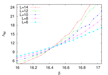
Figure 3: Reduced localization length of light atoms for $d=2$ and $U=9$. There is a critical inverse temperature $\beta_{c}^{\prime}\approx 16.5$, where an Anderson transition occurs.

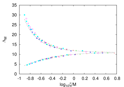
Figure 4: One parameter scaling for $d=2$ and $U=9$. The lower (upper) branch represents (de-) localized states. The data from the transfer-matrix calculation approach the scaling function of Eq. (10) with $\Lambda_{c}\approx 10.9$, $A\approx 0.09$ and $\nu\approx 0.88$ (dashed curves).

In conclusion, we have discussed a mixture of two fermionic species with different masses in an optical lattice, using the Falicov-Kimball model. The heavy atoms are represented as Ising spins and the light atoms as quantum particles. The latter tunnel in a random environment which is provided by a correlated distribution of heavy atoms. The distribution of the heavy atoms is given by an Ising-type model, which undergoes a second-order phase transition in $d=2$ from staggered order to disorder. Depending on the dimensionality ($d=1,2$) of the atomic system and the physical parameters (e.g. temperature or interaction strength), the quantum states of the light atoms are either localized or delocalized. All states of light atoms in a one-dimensional fermionic mixture are localized. In a two-dimensional mixture these states are localized at high temperatures and delocalized at low temperatures. Such a system can be realized experimentally as a mixture with two spin-polarized fermionic species.

References

- (1) S. Ospelkaus et al., Phys. Rev. Lett. 96, 180403 (2006)
- (2) G. Roati et al., Nature 453, 895 (2008)
- (3) J. Billy et al., Nature 453, 891 (2008)
- (4) P.W. Anderson, Phys. Rev. 109 1492 (1958)
- (5) F. Wegner, Z. Phys. B 25, 327 (1976)
- (6) E. Abrahams, P.W. Anderson, D.C. Licciardello, and T.V. Ramakrishnan, Phys. Rev. Lett. 42, 673 (1979)
- (7) C.A. Stan et al., Phys. Rev. Lett. 93, 143001 (2004); A. Mosk et al., Appl. Phys. B 73, 791 (2001); M. Zaccanti et al., Phys. Rev. A 74, 041605 (2006); E. Wille et al., Phys. Rev. Lett. 100, 053201 (2008)
- (8) U. Gavish and Y. Castin, Phys. Rev. Lett. 95, 020401 (2005)
- (9) C. Ates and K. Ziegler, Phys. Rev. A 71, 063610 (2005)
- (10) M.M. Máska et al., Phys. Rev. Lett. 101, 060404 (2008)
- (11) K. Ziegler, Phys. Rev. A 77, 013623 (2008)
- (12) K. Ziegler, Laser Physics 16, 699 (2006)
- (13) L.M. Falicov and J.C. Kimball, Phys. Rev. Lett. 22, 997 (1969)
- (14) P. Farkasovsky, Z. Phys. B 102, 91 (1997)
- (15) J.K. Freericks and V. Zlatić, Rev. Mod. Phys. 75, 1333 (2003)
- (16) A. MacKinnon and B. Kramer, Z.Phys. B 53, 1 (1983)
- (17) J.L. Pichard and G. Sarma, J. Phys. C 14, L127 (1981); K. Slevin and T. Ohtsuki, Phys. Rev. Lett. 82, 382 (1999)