Evidence of $WW+WZ$ production with lepton $+$ jets
final states in $p\bar{p}$ collisions at $\sqrt{s}=1.96$ TeV

Abstract

We present first evidence for $WW+WZ$ production in lepton+jets final states at a hadron collider. The data correspond to 1.07 fb^-1 of integrated luminosity collected with the D0 detector at the Fermilab Tevatron in $p\bar{p}$ collisions at $\sqrt{s}=1.96$ TeV. The observed cross section for $WW+WZ$ production is $20.2\pm 4.5$ pb, consistent with the standard model and more precise than previous measurements in fully leptonic final states. The probability that background fluctuations alone produce this excess is $<5.4\times 10^{-6}$, which corresponds to a significance of 4.4 standard deviations.

The production of vector-boson pairs in $p\bar{p}$ collisions ($WW$, $WZ$, or $ZZ$) provides important tests of the electroweak sector of the standard model (SM). The next-to-leading-order (NLO) cross sections for $WW$ and $WZ$ production in $p\bar{p}$ collisions at $\sqrt{s}=1.96$ GeV predicted by the SM are $\sigma(WW)=12.4\pm 0.8$ pb and $\sigma(WZ)=3.7\pm 0.3$ pb bib:Campbell . A discrepancy with this expectation or deviations in the predicted kinematic distributions could signal the presence of new physics, e.g., originating from anomalous trilinear gauge boson couplings bib:anocoups . The production of two weak bosons is also relevant to searches for the Higgs boson or for new particles in extensions of the SM. Production of $WW$ and $WZ$ in $p\bar{p}$ collisions at the Fermilab Tevatron Collider has thus far been observed only in fully leptonic decay modes bib:dz ; bib:cdf . Previous searches for $WW$ and $WZ$ in lepton+jets final states bib:D0RunI ; bib:CDFRunII , which benefit from a higher branching ratio relative to fully leptonic channels, were hindered by large backgrounds from jets produced in association with a $W$ boson ($W+$jets).

In this Letter we report first evidence from a hadron collider for the production of a $W$ boson that decays leptonically, associated with a second vector boson $V$ ($V$=$W$ or $Z$) that decays into $q\bar{q}$ ($WV$$\rightarrow\ell\nu q\bar{q};\ \,\ell$$=$$e,\mu$). The limited dijet mass resolution ($\approx$ 18% for dijets from $W/Z$ decays) results in a significant overlap of the $W$$\rightarrow q\bar{q}$ and $Z$$\rightarrow q\bar{q}$ dijet mass peaks. We therefore consider $WW$ and $WZ$ simultaneously, assuming the ratio of their cross sections as predicted by the SM. The use of improved multivariate event classification and new statistical techniques bib:poisson , as well as an increased integrated luminosity, make the $WV$ signal in lepton+jets final states more distinguishable from $W+$jets background and more accessible to measurement than in the past bib:D0RunI ; bib:CDFRunII . This analysis also provides a valuable proving ground for such advanced techniques, now ubiquitous in Higgs searches at the Tevatron.

We analyze 1.07 fb^-1 of data collected with the D0 detector bib:detector at a center-of-mass energy of 1.96 TeV at the Tevatron. Candidate $e\nu q\bar{q}$ events must pass a trigger based on a single electron or electron+jet(s) requirement that has an efficiency of $98^{+2}_{-3}$%. A suite of triggers for $\mu\nu q\bar{q}$ candidate events achieves an efficiency of $>95\%$ at 95% confidence level.

To select $WV$$\rightarrow\ell\nu q\bar{q}$ candidates, we require: a single reconstructed lepton (electron or muon) bib:leptons with transverse momentum $p_{T}>20$ GeV and pseudorapidity $|\eta|<1.1\ (2.0)$ for electrons (muons); the imbalance in transverse energy to be $E\kern-5.70007pt/_{T}>20$ GeV; and at least two jets bib:JetCone with $p_{T}>20$ GeV and $|\eta|<2.5$. The jet of highest $p_{T}$ must have $p_{T}>30$ GeV. To reduce background from processes that do not contain $W$$\rightarrow\ell\nu$, we require a “transverse” mass bib:smithUA1 of $M_{T}^{\ell\nu}>35$ GeV. The lepton must be spatially matched to a track reconstructed in the central tracker that originates from the primary vertex. Electrons (muons) must be isolated from other particles in the calorimeter (and central tracker) bib:iso .

Signal and background processes containing charged leptons are modeled via Monte Carlo (MC) simulation. The signal includes all possible $W$ and $Z$ decays, including their decays to leptons. The diboson signal (WW and WZ) is generated with pythia bib:PYTHIA using CTEQ6L parton distribution functions (PDFs). The fixed-order matrix element (FOME) generator alpgen bib:ALPGEN with CTEQ6L1 PDFs is used to generate $W+$jets, $Z+$jets, and $t\bar{t}$ events to leading order at the parton level. The FOME generator comphep bib:CompHEP is used to produce single top-quark MC samples. alpgen and comphep are interfaced to pythia for subsequent parton showering and hadronization. All simulated events undergo a geant-based bib:GEANT detector simulation and are reconstructed using the same programs as used for D0 data. The MC samples are normalized using next-to-leading-order (NLO) or next-to-next-to-leading-order predictions for SM cross sections, except $W+$jets  which is scaled to the data.

The probability for multijet events with misidentified leptons to pass all selection requirements is small; however, because of the copious production of multijet events, the background from this source cannot be ignored. For $\mu\nu q\bar{q}$, the multijet background is modeled with data that fail the muon isolation requirements, but pass all other selections. The normalization is determined from a fit to the $M_{T}^{\ell\nu}$ distribution. For $e\nu q\bar{q}$, the multijet background is estimated using a “loose-but-not-tight” data sample obtained by selecting events that pass loosened electron quality requirements, but fail the tight electron quality criteria bib:leptons . This sample is normalized by the probability for a jet that passes the “loose” electron requirements to also pass the tight requirement. Both $\mu\nu q\bar{q}$ and $e\nu q\bar{q}$ multijet samples are corrected for contributions from all processes modeled through MC.

Accurate modeling of the selected events is vital. The dominant background is $W+$jets, and the modeling of alpgen $W+$jets and sources of uncertainty are therefore studied in great detail. Comparison of alpgen with other generators and with data shows discrepancies bib:ALPGENcomp in jet $\eta$ and dijet angular separation. Data are used to correct these quantities in the alpgen $W+$jets and $Z+$jets samples. The possible bias in this procedure from the presence of the diboson signal in data is small, but is nevertheless taken into account via a systematic uncertainty. Systematic effects on the differential distributions of the alpgen $W$+jets and $Z$+jets MC events from changes of the renormalization and factorization scales and of the parameters used in the MLM parton-jet matching algorithm bib:MLM are also considered. Uncertainties on PDFs, as well as uncertainties from object reconstruction and identification, are evaluated for all MC samples. We consider the effect of systematic uncertainty both on the normalization and on the shape of differential distributions for signal and backgrounds bib:EPAPS .

The signal and the backgrounds are further separated using a multivariate classifier to combine information from several kinematic variables. This analysis uses a Random Forest (RF) classifier bib:SPR1 ; bib:SPR2 . Thirteen well-modeled kinematic variables bib:EPAPS that demonstrate a difference in probability density between signal and at least one of the backgrounds, such as dijet mass and $E\kern-5.70007pt/_{T}$, are used as inputs to the RF. The RF is trained using half of each MC sample. The other halves, along with the multijet background samples, are then evaluated by the RF and used in the measurement.

(a)
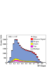
(b)

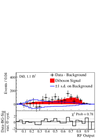
Figure 1: (a) The RF output distribution from the combined $e\nu q\bar{q}$ and $\mu\nu q\bar{q}$ channels for data and MC predictions following the fit of MC to data. (b) A comparison of the extracted signal (filled histogram) to background-subtracted data (points), along with the $\pm 1$ standard deviation (s.d.) systematic uncertainty on the background. The residual distance between the data points and the extracted signal, divided by the total uncertainty, is given at the bottom.

(a)
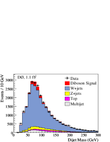
(b)

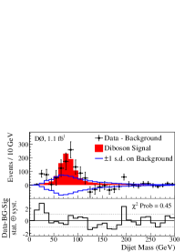
Figure 2: (a) The dijet mass distribution from the combined $e\nu q\bar{q}$ and $\mu\nu q\bar{q}$ channels for data and MC predictions following the fit to the RF output. (b) A comparison of the extracted signal (filled histogram) to background-subtracted data (points), along with the $\pm 1$ standard deviation (s.d.) systematic uncertainty on the background.The residual distance between the data points and the extracted signal, divided by the total uncertainty, is given at the bottom.

Table 1: Measured number of events for signal and each background after the combined fit (with total uncertainties determined from the fit) and the number observed in data.

	$e\nu q\bar{q}$ channel		$\mu\nu q\bar{q}$ channel
Diboson signal	436$\ \pm\$	36	527$\ \pm\$	43
$W$+jets	10100$\ \pm\$	500	11910$\ \pm\$	590
$Z$+jets	387$\ \pm\$	61	1180$\ \pm\$	180
$t\bar{t}$ + single top	436$\ \pm\$	57	426$\ \pm\$	54
Multijet	1100$\ \pm\$	200	328$\ \pm\$	83
Total predicted	12460$\ \pm\$	550	14370$\ \pm\$	620
Data	12473		14392

Table 2: The signal cross section extracted from a simultaneous fit of the $WV$ cross section and the normalization factor for $W+$jets. Also given are expected and observed p-values obtained by comparing the measurement with pseudo-experiments assuming no signal and the corresponding significance in number of standard deviations (s.d.) for a one-sided Gaussian integral.

Channel	Fitted signal $\sigma$ (pb)	Expected p-value (significance)	Observed p-value (significance)
$e\nu q\bar{q}$ RF Output	18.0$\pm$3.7(stat)$\pm$5.2(sys)$\pm$1.1(lum)	$6.8\times 10^{-3}$ (2.5 s.d.)	$3.2\times 10^{-3}$ (2.7 s.d.)
$\mu\nu q\bar{q}$ RF Output	22.8$\pm$3.3(stat)$\pm$4.9(sys)$\pm$1.4(lum)	$1.8\times 10^{-3}$ (2.9 s.d.)	$5.2\times 10^{-5}$ (3.9 s.d.)
Combined RF Output	20.2$\pm$2.5(stat)$\pm$3.6(sys)$\pm$1.2(lum)	$1.5\times 10^{-4}$ (3.6 s.d.)	$5.4\times 10^{-6}$ (4.4 s.d.)
Combined Dijet Mass	18.5$\pm$2.8(stat)$\pm$4.9(sys)$\pm$1.1(lum)	$1.7\times 10^{-3}$ (2.9 s.d.)	$4.4\times 10^{-4}$ (3.3 s.d.)

The signal cross section is determined from a fit of signal and background RF templates to the data by minimizing a Poisson $\chi^{2}$ function with respect to variations in the systematic uncertainties bib:poisson . The magnitude of systematic uncertainties is effectively constrained by the regions of the RF distribution with low signal over background. A Gaussian prior is used for each systematic uncertainty. Different uncertainties are assumed to be mutually independent, but those common to multiple samples or lepton channels are assumed to be 100% correlated.

The fit simultaneously varies the $WV$ and $W+$jets contributions, thereby also determining the normalization factor for the $W+$jets MC sample. This obviates the need for using the predicted alpgen cross section, and provides a more rigorous approach that incorporates an unbiased uncertainty from $W+$jets when extracting the $WV$ cross section. The normalization factor from the fit for the $W$+jets component is $1.53\pm 0.13$, similar to the expected ratio of NLO to LO cross sections bib:Campbell2 . The measured yields for signal and each background are given in Table 1. Table 2 contains the measured $WV$ cross section for each channel, separately and combined, showing consistent results between channels and the SM prediction of $\sigma(WV)=16.1\pm 0.9$ pb bib:Campbell . The combined fit yields a cross section of 20.2 $\pm$ 2.5(stat) $\pm$ 3.6(sys) $\pm$ 1.2(lum) pb. The RF output distributions following the combined fit are shown in Fig. 1, along with comparisons of consistency between the background-subtracted data and the extracted signal. Figure 2 shows analogous plots for the dijet mass after the combined fit to the RF output. The dominant systematic uncertainties arise from the modeling of the $W$+jets background and the jet energy scale, contributing 2.4 pb and 1.9 pb to the total systematic uncertainty bib:EPAPS , respectively. The position of the dijet mass peaks in data and MC are consistent within one half standard deviation, which includes the relative data/MC uncertainty in energy scale. As a cross check, we also perform the measurement using only the dijet mass distribution. The result, also given in Table 2, although less precise, is consistent with that obtained using the RF output.

The significance of the measurement is obtained via fits of the signal+background hypothesis to pseudo-data samples drawn from the background-only hypothesis bib:singleTop . The observed (or expected) significance corresponds to the fraction of outcomes that yield a $WV$ cross section at least as large as that measured in data (as predicted by the SM). The probabilities that background fluctuations could produce the expected and observed signal in each channel (p-values), separately and combined, are shown in Table 2, along with their corresponding significance (equivalent one-sided Gaussian probabilities). The $\chi^{2}$ fit with respect to variations in the systematic uncertainties bib:poisson results in an improvement of the expected significance of the result from 2.4 (1.6) to 3.6 (2.9) standard deviations when using the RF output (dijet mass) discriminant.

In summary, we measure $\sigma(WV)=20.2\pm 4.5$ pb (with $V$=$W$ or $Z$) in $p\bar{p}$ collisions at $\sqrt{s}=1.96$ TeV. The probability that the backgrounds fluctuate to give an excess as large as observed in data is $<5.4\times 10^{-6}$, corresponding to a significance of 4.4 standard deviations. This represents the first evidence for $WV$ production in lepton+jets events at a hadron collider. The result is more precise than previous independent measurements of $WW$ and $WZ$ yields in fully leptonic final states bib:dz ; bib:cdf and consistent with the SM prediction of $\sigma(WV)=16.1\pm 0.9$ pb bib:Campbell . This work clearly demonstrates the ability of the D0 experiment to isolate a small signal in a large background in a final state of direct relevance to searches for a low mass Higgs, and thereby validates the analytical methods used in searches for Higgs bosons at the Tevatron bib:tevcombo .

We thank the staffs at Fermilab and collaborating institutions, and acknowledge support from the DOE and NSF (USA); CEA and CNRS/IN2P3 (France); FASI, Rosatom and RFBR (Russia); CNPq, FAPERJ, FAPESP and FUNDUNESP (Brazil); DAE and DST (India); Colciencias (Colombia); CONACyT (Mexico); KRF and KOSEF (Korea); CONICET and UBACyT (Argentina); FOM (The Netherlands); STFC (United Kingdom); MSMT and GACR (Czech Republic); CRC Program, CFI, NSERC and WestGrid Project (Canada); BMBF and DFG (Germany); SFI (Ireland); The Swedish Research Council (Sweden); CAS and CNSF (China); and the Alexander von Humboldt Foundation (Germany).

Supplemental Material:

I Systematic Uncertainties

Table 3 gives the % systematic uncertainties for Monte Carlo simulations and multijet estimates. We consider the effect of systematic uncertainty both on the normalization and on the shape of differential distributions for signal and backgrounds. Although Table 3 lists an uncertainty for the $W$+jets simulation, this uncertainty is not used when measuring the diboson signal cross section, for which the $W$+jets normalization is a free parameter. However, the size of the uncertainty must be specified for generating the pseudo-data used in the estimation of significance. Also in the table is the contribution of each systematic uncertainty to the total systematic uncertainty of 3.6 pb on the measured cross section, $\sigma^{\mathrm{meas}}(WV)$. This total systematic uncertainty is obtained from the systematic uncertainties on the parameter in the fit to the Random Forest (RF) output, $\sigma^{\mathrm{meas}}(WV)$/$\sigma^{\mathrm{th}}(WV)$, by multiplying each contribution by the theoretical cross section $\sigma^{\mathrm{th}}(WV)$. The additional uncertainty on the integrated luminosity for data (6.1%) is therefore considered separately.

Table 3: The % systematic uncertainties for Monte Carlo simulations and multijet estimates. Uncertainties are identical for both lepton channels except where otherwise indicated. The nature of the uncertainty, i.e., whether it refers to a differential dependence (D) or just normalization (N), is also provided. The values for uncertainties with a differential dependence correspond to the maximum amplitude of fluctuations in the RF output. Also provided is the contribution of each source to the total systematic uncertainty of 3.6 pb on the measured cross section, which does not include the additional uncertainty of 6.1% for the luminosity.

Source of systematic	Diboson signal		$W$+jets		$Z$+jets		Top		Multijet		Nature	$\Delta\sigma\;(pb)$
uncertainty
Trigger efficiency, $e\nu q\bar{q}$ channel		$+2/-3$		$+2/-3$		$+2/-3$		$+2/-3$			N	$<0.1$
Trigger efficiency, $\mu\nu q\bar{q}$ channel		$+0/-5$		$+0/-5$		$+0/-5$		$+0/-5$			D	$<0.1$
Lepton identification		$\pm$4		$\pm$4		$\pm$4		$\pm$4			N	$<0.1$
Jet identification		$\pm$1		$\pm$1		$\pm$1		$\pm<$1			D	0.3
Jet energy scale		$\pm$4		$\pm$9		$\pm$9		$\pm$4			D	1.9
Jet energy resolution		$\pm$3		$\pm$4		$\pm$4		$\pm$4			N	$<0.1$
Cross section				$\pm$20		$\pm$6		$\pm$10			N	1.1
Multijet normalization, $e\nu q\bar{q}$ channel										$\pm$20	N	0.9
Multijet normalization, $\mu\nu q\bar{q}$ channel										$\pm$30	N	0.5
Multijet shape, $e\nu q\bar{q}$ channel										$\pm$6	D	$<0.1$
Multijet shape, $\mu\nu q\bar{q}$ channel										$\pm$10	D	$<0.1$
Diboson signal NLO/LO shape		$\pm$10									D	$<0.1$
Parton distribution function		$\pm$1		$\pm$1		$\pm$1		$\pm$1			D	0.2
alpgen $\eta$ and $\Delta R$ corrections				$\pm$1		$\pm$1					D	$<0.1$
Renormalization and factorization scale				$\pm$3		$\pm$3					D	0.9
alpgen parton-jet matching parameters				$\pm$4		$\pm$4					D	2.4

II Input Variables to the Random Forest Classifier

The 13 kinematic variables used in the RF classifier are listed below, and their distributions are shown in Fig. 3. The variables are derived from characteristics of objects reconstructed from observables in each event and can be loosely classified into three categories: (i) variables based on the kinematics of individual objects, (ii) variables based on the kinematics of multiple objects, and (iii) variables based on the angular relationships among objects. Several variables are calculated using the four-momentum of the dijet system or the leptonic $W$ candidate ($W^{\ell\nu}$). The dijet system is defined as the four-momentum sum of the jets with highest $p_{T}$ (jet₁) and second highest $p_{T}$ (jet₂). $W^{\ell\nu}$ is reconstructed from the charged lepton and the $E\kern-5.70007pt/_{T}$. The neutrino from the $W$$\to\ell\nu$ decay is assigned the transverse momentum defined by $E\kern-5.70007pt/_{T}$  and a longitudinal momentum that is calculated assuming the mass of the W for $\ell\nu$ ($M_{W}=80.4$ GeV). Of the two possible solutions, we choose the one that provides the smaller total invariant mass of all objects in the event.

• Kinematics of Individual Objects:

  1. The imbalance in transverse energy ($E\kern-5.70007pt/_{T}$), which is defined by the imbalance in transverse momentum as determined from the summing of products of energies and cosines of polar angles of calorimeter cells relative to the center of the detector (corrected for transverse momenta of muons and energy scales for jets and electrons in the event).

  2. The jet with second highest $p_{T}$: $p_{T}(\mathrm{Jet}_{2})$.

• Kinematics of Multiple Objects:

  1. The “transverse $W$ mass” reconstructed from the charged lepton and the $E\kern-5.70007pt/_{T}$: $M_{T}^{\ell\nu}=\sqrt{2\;p_{T}^{\ell}\;E\kern-5.70007pt/_{T}\;(1-\cos(\Delta\phi(\ell,E\kern-5.70007pt/_{T})))}$.

  2. The $p_{T}$ of the $W^{\ell\nu}$ candidate.

  3. The invariant mass of the dijet system.

  4. The magnitude of the leading jet momentum perpendicular to the plane of the dijet system: $\frac{|\vec{p}_{T}(\mathrm{Jet}_{1}+\mathrm{Jet}_{2})\times\vec{p}_{T}(\mathrm{Jet}_{1})|}{|\vec{p}_{T}(\mathrm{Jet}_{1}+\mathrm{Jet}_{2})|}$, where “$\times$” represents the usual vector cross product. This variable is calculated in the rest frame of the $W^{\ell\nu}$ candidate and is denoted $p_{T}^{Rel}(\mathrm{Dijet},\mathrm{Jet}_{1}))^{\mathrm{WFrame}}$.

  5. The magnitude of the second-leading jet momentum perpendicular to the plane of the dijet system: $\frac{|\vec{p}_{T}(\mathrm{Jet}_{1}+\mathrm{Jet}_{2})\times\vec{p}_{T}(\mathrm{Jet}_{2})|}{|\vec{p}_{T}(\mathrm{Jet}_{1}+\mathrm{Jet}_{2})|}$. This variable is calculated in the laboratory frame and is denoted $p_{T}^{Rel}(\mathrm{Dijet},\mathrm{Jet}_{2}))^{\mathrm{LabFrame}}$.

  6. The angular separation between the two jets of highest $p_{T}$, weighted by the ratio of the transverse momentum of the second-leading jet and the $W^{\ell\nu}$ candidate: $\Delta R(\mathrm{Jet}_{1},\mathrm{Jet}_{2})\frac{p_{T}(\mathrm{Jet}_{2})}{p_{T}(\ell)+E\kern-3.99005pt/_{T}}$. This variable is calculated in the rest frame of the $W^{\ell\nu}$ candidate and is denoted $k_{T}^{\mathrm{Min,WFrame}}$.

  7. The “centrality” of the charged lepton and jets system, defined as the scalar sum of transverse momenta divided by the sum of energies of the charged lepton and all jets in the event.

• Angular Relationships of Objects:

  1. The azimuthal separation between the charged lepton and the $E\kern-5.70007pt/_{T}$  vector: $\Delta\phi(E\kern-5.70007pt/_{T},lepton)$.

  2. The cosine of the angle between the dijet system and the leading jet in the laboratory frame: $\cos(\angle(\mathrm{Dijet},\mathrm{Jet}_{1}))$.

  3. The cosine of the angle between the dijet system and the second-leading jet in the laboratory frame: $\cos(\angle(\mathrm{Dijet},\mathrm{Jet}_{2}))$.

  4. Cosine of the angle between leading jet and the $W^{\ell\nu}$ candidate: $\cos(\angle(W^{\ell\nu},\mathrm{Jet}_{1}))^{\mathrm{DijetFrame}}$, evaluated in the rest frame of the dijet system.

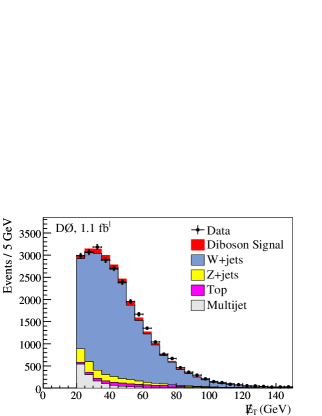
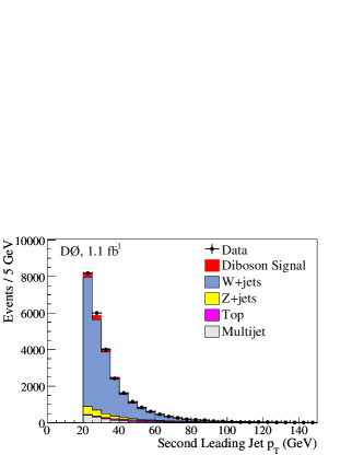
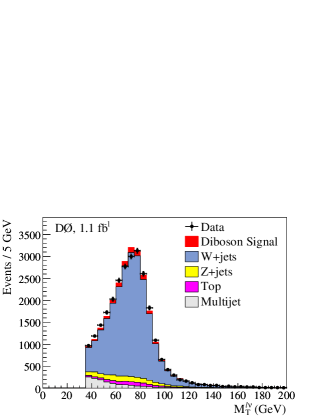
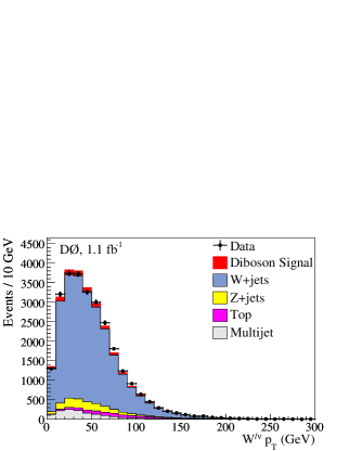
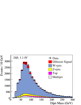
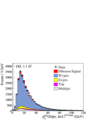
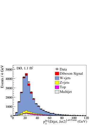
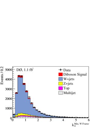
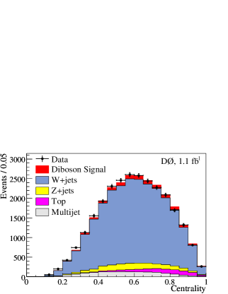
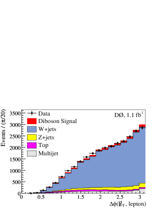
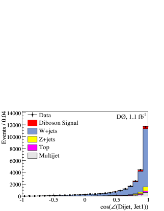
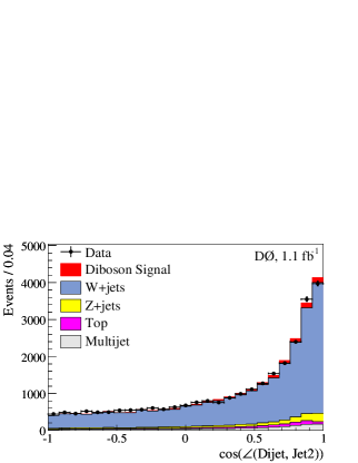
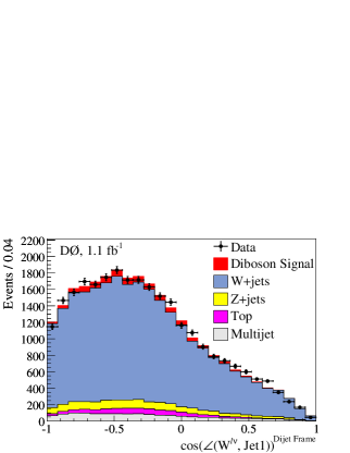
Figure 3: Distributions of the RF input variables for the combined $e\nu q\bar{q}$ and $\mu\nu q\bar{q}$ channels comparing the data with the MC predictions, following the fit of MC to data.

III Correlation between Dijet Invariant Mass and RF Output

There is a high degree of correlation between the dijet invariant mass and the RF output. This can be observed in the dijet invariant mass distributions for events with low, intermediate and high values for the RF output shown in Fig. 4. As expected, events in the low region of the RF output correspond to the background dominated sidebands of the dijet invariant mass distribution and events in the high region of the RF output correspond to the signal resonance region of the dijet invariant mass. The purity of the signal in the dijet invariant mass distribution is enhanced for high values of the RF output because a substantial fraction of the background events in the dijet invariant mass signal region has been moved to the intermediate region of the RF output.

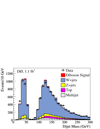
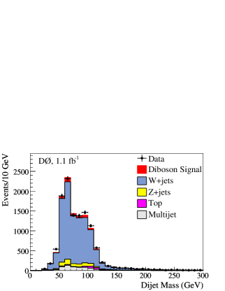
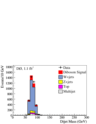
(a)	(b)	(c)

Figure 4: Distributions of the dijet invariant mass for the combined $e\nu q\bar{q}$ and $\mu\nu q\bar{q}$ channels comparing the data with the MC predictions for events in three regions of the RF output: (a) $0\leq$ RF output $\leq 0.33$, (b) $0.33<$ RF output $\leq 0.66$ and (c) $0.66<$ RF output $\leq 1$.

References

- (1)
- (2) Visitor from Augustana College, Sioux Falls, SD, USA.
- (3) Visitor from Rutgers University, Piscataway, NJ, USA.
- (4) Visitor from The University of Liverpool, Liverpool, UK.
- (5) Visitor from II. Physikalisches Institut, Georg-August-University, Göttingen, Germany.
- (6) Visitor from Centro de Investigacion en Computacion - IPN, Mexico City, Mexico.
- (7) Visitor from ECFM, Universidad Autonoma de Sinaloa, Culiacán, Mexico.
- (8) Visitor from Helsinki Institute of Physics, Helsinki, Finland.
- (9) Visitor from Universität Bern, Bern, Switzerland.
- (10) Visitor from Universität Zürich, Zürich, Switzerland.
- (11) Deceased.
- (12) J. M. Campbell and R. K. Ellis, Phys. Rev. D 60, 113006 (1999). Cross sections were calculated with the same parameter values given in the paper, except with TeV.
- (13) K. Hagiwara, S. Ishihara, R. Szalapski and D. Zeppenfeld, Phys. Rev. D 48 (1993).
- (14) D0 Collaboration: V. M. Abazov et al., Phys. Rev. Lett. 94, 151801 (2005); Phys. Rev. D 76, 111104(R) (2007); Phys. Rev. Lett. 101, 171803 (2008).
- (15) CDF Collaboration: D. Acosta et al., Phys. Rev. Lett. 94, 211801 (2005); A. Abulencia et al., Phys. Rev. Lett. 98, 161801 (2007); T. Aaltonen et al., Phys. Rev. Lett. 100, 201801 (2008).
- (16) B. Abbott et al. (D0 Collaboration), Phys. Rev. D 62, 052005 (2000).
- (17) T. Aaltonen et al. (CDF Collaboration), Phys. Rev. D 76, 111103(R) (2007).
- (18) W. Fisher, FERMILAB-TM-2386-E (2006).
- (19) B. Abbott et al. (D0 Collaboration), Nucl. Instrum. Methods Phys. Res. A 565, 463 (2006).
- (20) V. M. Abazov et al. (D0 Collaboration), Phys. Lett. B 626, 45 (2005).
- (21) G. C. Blazey et al., arXiv:hep-ex/0005012 (2000). The seeded cone algorithm with radius 0.5 was used.
- (22) J. Smith, W. L. van Neerven, and J. A. M. Vermaseren, Phys. Rev. Lett. 50, 1738 (1983).
- (23) V. M. Abazov et al. (D0 Collaboration), Phys. Rev. Lett. 100, (2008).
- (24) T. Sjöstrand et al., Comput. Phys. Commun. 135, 238 (2001). Verison 6.3 was used.
- (25) M. L. Mangano et al., JHEP 0307, 001 (2003). Version 2.05 was used.
- (26) A. Pukhov et al., arXiv:hep-ph/9908288 (2000).
- (27) R. Brun, F. Carminati, CERN Program Library Long Writeup W5013 (1993).
- (28) J. Alwall et al., Eur. Phys. C 53, 473 (2008).
- (29) S. Höche et al., arXiv:hep-ph/0602031 (2006).
- (30) See attached supplemental material.
- (31) L. Breiman, Machine Learning 45, 5 (2001).
- (32) I. Narsky, arXiv:physics/0507143 [physics.data-an] (2005).
- (33) J. M. Campbell and R. K. Ellis, Phys. Rev. D 65, 113007 (2002).
- (34) V. M. Abazov et al. (D0 Collaboration), Phys. Rev. D 78, 012005 (2008).
- (35) TEVNPH Working Group, for the CDF Collaboration and D0 Collaboration, arXiv:0804.3423 [hep-ex] (2008).