Multistage Hypothesis Tests for the Mean of a Normal Distribution

Abstract

In this paper, we have developed new multistage tests which guarantee prescribed level of power and are more efficient than previous tests in terms of average sampling number and the number of sampling operations. Without truncation, the maximum sampling numbers of our testing plans are absolutely bounded. Based on geometrical arguments, we have derived extremely tight bounds for the operating characteristic function. To reduce the computational complexity for the relevant integrals, we propose adaptive scanning algorithms which are not only useful for present hypothesis testing problem but also for other problem areas.

1 Introduction

Consider a Gaussian random variable $X$ with mean $\mu$ and variance $\sigma^{2}$. In many applications, it is an important problem to determine whether the mean $\mu$ is less or greater than a prescribed value $\gamma$ based on i.i.d. random samples $X_{1},X_{2},\cdots$ of $X$. Such problem can be put into the setting of testing hypothesis $\mathscr{H}_{0}:\mu\leq\mu_{0}$ versus $\mathscr{H}_{1}:\mu>\mu_{1}$ with $\mu_{0}=\gamma-\varepsilon\sigma$ and $\mu_{1}=\gamma+\varepsilon\sigma$, where $\varepsilon$ is a positive number specifying the width of the indifference zone $(\mu_{0},\mu_{1})$. It is usually required that the size of the Type I error is no greater than $\alpha\in(0,1)$ and the size of the Type II error is no greater than $\beta\in(0,1)$. That is,

$$\Pr\left\{\text{Reject}\;\mathscr{H}_{0}\mid\mu\right\}\leq\alpha,\quad\forall\mu\in(-\infty,\mu_{0}]$$ (1)

$$\Pr\left\{\text{Accept}\;\mathscr{H}_{0}\mid\mu\right\}\leq\beta,\quad\forall\mu\in[\mu_{1},\infty).\;$$ (2)

The hypothesis testing problem described above has been extensively studied in the framework of sequential probability ratio test (SPRT), which was established by Wald [5] during the period of second world war of last century. The SPRT suffers from several drawbacks. First, the sampling number of SPRT is a random number which is not bounded. However, to be useful, the maximum sampling number of any testing plan should be bounded by a deterministic number. Although this can be fixed by forced termination (see, e.g., [4] and the references therein), the prescribed level of power may not be ensured as a result of truncation. Second, the number of sampling operations of SPRT is as large as the number of samples. In practice, it is usually much more economical to take a batch of samples at a time instead of one by one. Third, the efficiency of SPRT is optimal only for the endpoints of the indifference zone. For other parametric values, the SPRT can be extremely inefficient. Needless to say, a truncated version of SPRT may suffer from the same problem due to the partial use of the boundary of SPRT. Third, when the variance $\sigma^{2}$ is not available, a weighting function needs to be constructed so that the testing problem can be fit into the framework of SPRT. The construction of such weighting function is a difficult task and severely limit the efficiency of the resultant test plan.

In this paper, to overcome the limitations of existing tests for the mean of a normal distribution, we have established a new class testing plans having the following features: i) The testing has a finite number of stages and thus the cost of sampling operations is reduced as compared to SPRT. ii) The sampling number is absolutely bounded without truncation. iii) The prescribed level of power is rigorously guaranteed. iv) The testing is not only efficient for the endpoints of indifference zone, but also efficient for other parametric values. v) Even the variance $\sigma^{2}$ is unknown, our test plans do not require any weighting function.

In general, our testing plans consist of $s$ stages. For $\ell=1,\cdots,s$, the sample size of the $\ell$-th stage is $n_{\ell}$. For the $\ell$-th stage, a decision variable $\boldsymbol{D}_{\ell}$ is defined by using samples $X_{1},\cdots,X_{n_{\ell}}$ such that $\boldsymbol{D}_{\ell}$ assumes only three possible values $0,\;1$ and $2$ with the following notion:

(i) Sampling is continued until $\boldsymbol{D}_{\ell}\neq 0$ for some $\ell\in\{1,\cdots,s\}$. Since the sampling must be terminated at or before the $s$-th stage, it is required that $\boldsymbol{D}_{s}\neq 0$. For simplicity of notations, we also define $\boldsymbol{D}_{0}=0$.

(ii) The null hypothesis $\mathscr{H}_{0}$ is accepted at the $\ell$-th stage if $\boldsymbol{D}_{\ell}=1$ and $\boldsymbol{D}_{i}=0$ for $1\leq i<\ell$.

(iii) The null hypothesis $\mathscr{H}_{0}$ is rejected at the $\ell$-th stage if $\boldsymbol{D}_{\ell}=2$ and $\boldsymbol{D}_{i}=0$ for $1\leq i<\ell$.

As will be seen in the our specific testing plans, the sample sizes $n_{1}<n_{2}<\cdots,n_{s}$ and decision variables $\boldsymbol{D}_{1},\cdots,\boldsymbol{D}_{s}$ depend on the parameters $\alpha,\;\beta,\;\mu_{0},\;\mu_{1}$ and other parameters such as the risk tuning parameter $\zeta$ and the sample size incremental factor $\rho$. The requirements of power can be satisfied by determining an appropriate value of $\zeta$ via bisection search. For this purpose, we have derived, by a geometrical approach, readily computable bounds for the evaluation of the operating characteristic (OC) function.

The remainder of the paper is organized as follows. In Section 2, we present our approach for testing the mean of a normal distribution in the context of knowing the variance $\sigma^{2}$. In Section 3, we describe our method for for testing the mean of a normal distribution for situations that the variance $\sigma^{2}$ is not available. Section 4 discusses the evaluation of OC functions. In Section, we propose adaptive scanning algorithms for integration, summation, zero finding and optimization. These new methods are useful for our current problem and other problem areas. Section 6 is the conclusion. All proofs of theorems are given in Appendices.

Throughout this paper, we shall use the following notations. The ceiling function is denoted by $\lceil.\rceil$ (i.e., $\lceil x\rceil$ represents the smallest integer no less than $x$). The gamma function is denoted by $\Gamma(.)$. The inverse cosine function taking values on $[0,\pi]$ is denoted by $\arccos(.)$. The inverse tangent function taking values on $\left[-\frac{\pi}{2},\frac{\pi}{2}\right]$ is denoted by $\arctan(.)$. We use the notation $\Pr\{.\mid\theta\}$ to indicate that the associated random samples $X_{1},X_{2},\cdots$ are parameterized by $\theta$. The parameter $\theta$ in $\Pr\{.\mid\theta\}$ may be dropped whenever this can be done without introducing confusion. The other notations will be made clear as we proceed.

2 Testing the Mean of a Normal Distribution with Known Variance

For $\delta\in(0,1)$, let $\mathcal{Z}_{\delta}>0$ be the critical value of a normal distribution with zero mean and unit variance, i.e., $\Phi(\mathcal{Z}_{\delta})=\frac{1}{\sqrt{2\pi}}\int_{\mathcal{Z}_{\delta}}^{\infty}e^{-\frac{x^{2}}{2}}dx=\delta$. In situations that the variance $\sigma^{2}$ is known, our testing plan, developed in [3], is described as follows.

Theorem 1

Let $\zeta>0$ and $\rho>0$. Let $n_{1}<n_{2}<\cdots<n_{s}$ be the ascending arrangement of all distinct elements of $\left\{\left\lceil\frac{(\mathcal{Z}_{\zeta\alpha}+\mathcal{Z}_{\zeta\beta})^{2}}{4\varepsilon^{2}}(1+\rho)^{i-\tau}\right\rceil:i=1,\cdots,\tau\right\}$, where $\tau$ is a positive integer. Define $a_{\ell}=\varepsilon\sqrt{n_{\ell}}-\mathcal{Z}_{\zeta\beta},\;b_{\ell}=\mathcal{Z}_{\zeta\alpha}-\varepsilon\sqrt{n_{\ell}}$ for $\ell=1,\cdots,s-1$, and $a_{s}=b_{s}=\frac{\mathcal{Z}_{\zeta\alpha}-\mathcal{Z}_{\zeta\beta}}{2}$. Define

$$\overline{X}_{n_{\ell}}=\frac{\sum_{i=1}^{n_{\ell}}X_{i}}{n_{\ell}},\qquad T_{\ell}=\frac{\sqrt{n_{\ell}}\;(\overline{X}_{n_{\ell}}-\gamma)}{\sigma},\qquad\boldsymbol{D}_{\ell}=\begin{cases}1&\text{for}\;T_{\ell}\leq a_{\ell},\\ 2&\text{for}\;T_{\ell}>b_{\ell},\\ 0&\text{else}\end{cases}$$

for $\ell=1,\cdots,s$. Then, both (1) and (2) are guaranteed provided that $0<\zeta\leq\frac{1}{\tau}$. Moreover, the OC function $\Pr\left\{\text{Accept}\;\mathscr{H}_{0}\mid\mu\right\}$ is monotonically decreasing with respect to $\mu\in(-\infty,\mu_{0})\cup(\mu_{1},\infty)$.

To compute tight bounds for the OC function, we have the following result.

Theorem 2

Let $U$ and $V$ be independent Gaussian random variables with zero mean and variance unity. Define

$$\varphi(\theta,\zeta,\alpha,\beta) = \Phi\left(\sqrt{n_{1}}\theta-b_{1}\right)+\sum_{\ell=2}^{s}\Pr\left\{b_{\ell}-\sqrt{n_{\ell}}\theta\leq U\leq k_{\ell}V-\sqrt{n_{\ell}}\theta+\sqrt{\frac{n_{\ell}}{n_{\ell-1}}}b_{\ell-1}\right\}$$

$$-\;\sum_{\ell=2}^{s}\Pr\left\{b_{\ell}-\sqrt{n_{\ell}}\theta\leq U\leq k_{\ell}V-\sqrt{n_{\ell}}\theta+\sqrt{\frac{n_{\ell}}{n_{\ell-1}}}a_{\ell-1}\right\}$$

with $k_{\ell}=\sqrt{\frac{n_{\ell}}{n_{\ell-1}}-1},\;\ell=2,\cdots,s$. Then, $\Pr\{\text{Accept}\;\mathscr{H}_{0}\mid\mu=\theta\sigma+\gamma\}>1-\varphi(\theta,\zeta,\alpha,\beta)$ for any $\theta\in(-\infty,-\varepsilon]$ and $\Pr\{\text{Accept}\;\mathscr{H}_{0}\mid\mu=\theta\sigma+\gamma\}<\varphi(-\theta,\zeta,\beta,\alpha)$ for any $\theta\in[\varepsilon,\infty)$.

See Appendix A for a proof.

As can be seen from the proof of Theorem 2, we have $\sum_{\ell=1}^{s}\Pr\{\boldsymbol{D}_{\ell-1}=0,\;\boldsymbol{D}_{\ell}=2\mid\mu_{0}\}=\varphi(\frac{\mu_{0}-\gamma}{\sigma},\zeta,\alpha,\beta)$ and $\sum_{\ell=1}^{s}\Pr\{\boldsymbol{D}_{\ell-1}=0,\;\boldsymbol{D}_{\ell}=1\mid\mu_{1}\}=\varphi(\frac{\gamma-\mu_{1}}{\sigma},\zeta,\beta,\alpha)$. By making use of such results and a bisection search method, we can determine an appropriate value of $\zeta$ so that both (1) and (2) are guaranteed.

With regard to the distribution of sample number $\mathbf{n}$, we have, for $\ell=1,\cdots,s-1$,

$$\Pr\{\mathbf{n}>n_{\ell}\} \leq \Pr\left\{a_{\ell}<T_{\ell}\leq b_{\ell}\right\}=\Pr\left\{T_{\ell}\leq b_{\ell}\right\}-\Pr\left\{T_{\ell}\leq a_{\ell}\right\}$$

$$= \Pr\left\{U+\theta\sqrt{n_{\ell}}\leq b_{\ell}\right\}-\Pr\left\{U+\theta\sqrt{n_{\ell}}\leq a_{\ell}\right\}=\Phi\left(b_{\ell}-\sqrt{n_{\ell}}\theta\right)-\Phi\left(a_{\ell}-\sqrt{n_{\ell}}\theta\right),$$

where $U$ is a Gaussian random variable with zero mean and unit variance.

3 Testing the Mean of a Normal Distribution with Unknown Variance

For $\delta\in(0,1)$, let $t_{n,\delta}$ be the critical value of Student’s $t$-distribution with $n$ degrees of freedom. Namely, $t_{n,\delta}$ is a number satisfying

$$\int_{t_{n,\delta}}^{\infty}\frac{\Gamma(\frac{n+1}{2})}{\sqrt{n\pi}\;\Gamma(\frac{n}{2})}\left(1+\frac{x^{2}}{n}\right)^{-\frac{n+1}{2}}=\delta.$$

In situations that the variance $\sigma^{2}$ is unknown, our testing plan, developed in [3], is described as follows.

Theorem 3

Let $\zeta>0$ and $\rho>0$. Let $n^{*}$ be the minimum integer $n$ such that $t_{n-1,\zeta\alpha}+t_{n-1,\zeta\beta}\leq 2\varepsilon\sqrt{n-1}$. Let $n_{1}<n_{2}<\cdots<n_{s}$ be the ascending arrangement of all distinct elements of $\{\lceil n^{*}\;(1+\rho)^{i-\tau}\rceil:i=1,\cdots,\tau\}$, where $\tau$ is a positive integer. Define $a_{\ell}=\varepsilon\sqrt{n_{\ell}-1}-t_{n_{\ell}-1,\zeta\beta},\;b_{\ell}=t_{n_{\ell}-1,\zeta\alpha}-\varepsilon\sqrt{n_{\ell}-1}$ for $\ell=1,\cdots,s-1$, and $a_{s}=b_{s}=\frac{t_{n_{s}-1,\zeta\alpha}-t_{n_{s}-1,\zeta\beta}}{2}$. Define

$$\overline{X}_{n_{\ell}}=\frac{\sum_{i=1}^{n_{\ell}}X_{i}}{n_{\ell}},\quad\widehat{\sigma}_{n_{\ell}}=\sqrt{\frac{\sum_{i=1}^{n_{\ell}}(X_{i}-\overline{X}_{n_{\ell}})^{2}}{n_{\ell}-1}},\quad\widehat{T}_{\ell}=\frac{\sqrt{n_{\ell}}(\overline{X}_{n_{\ell}}-\gamma)}{\widehat{\sigma}_{n_{\ell}}},\quad\boldsymbol{D}_{\ell}=\begin{cases}1&\text{for}\;\widehat{T}_{\ell}\leq a_{\ell},\\ 2&\text{for}\;\widehat{T}_{\ell}>b_{\ell},\\ 0&\text{else}\end{cases}$$

for $\ell=1,\cdots,s$. Then, both (1) and (2) are guaranteed if $\zeta>0$ is sufficiently small. Moreover, the OC function $\Pr\left\{\text{Accept}\;\mathscr{H}_{0}\mid\mu\right\}$ is monotonically decreasing with respect to $\mu\in(-\infty,\mu_{0})\cup(\mu_{1},\infty)$.

To obtain tight bounds for the OC function, the following result is useful.

Theorem 4

Let $U,\;V$ and $Y_{\ell},\;Z_{\ell},\;\ell=2,\cdots,s$ be independent random variables such that $U,\;V$ possess identical normal distributions with zero mean and unit variance and that $Y_{\ell},\;Z_{\ell}$ possess chi-square distributions of $n_{\ell-1}-1$ and $n_{\ell}-n_{\ell-1}-1$ degrees of freedom respectively. Define $k_{\ell}=\sqrt{\frac{n_{\ell}}{n_{\ell-1}}-1},\;c_{\ell}=\frac{a_{\ell}}{\sqrt{n_{\ell}-1}}$ and $d_{\ell}=\frac{b_{\ell}}{\sqrt{n_{\ell}-1}}$ for $\ell=1,\cdots,s$. Define $\mathcal{P}(\theta,\zeta,\alpha,\beta)=\sum_{\ell=1}^{s}\mathcal{P}_{\ell}$ where $\mathcal{P}_{1}=\Pr\left\{\widehat{T}_{1}>b_{1}\right\}$ and

$$\mathcal{P}_{\ell}=\begin{cases}\Pr\left\{d_{\ell}\sqrt{V^{2}+Y_{\ell}+Z_{\ell}}<U+\sqrt{n_{\ell}}\theta\leq k_{\ell}V+d_{\ell-1}\sqrt{\frac{n_{\ell}Y_{\ell}}{n_{\ell-1}}}\right\}\\ -\;\Pr\left\{d_{\ell}\sqrt{V^{2}+Y_{\ell}+Z_{\ell}}<U+\sqrt{n_{\ell}}\theta\leq k_{\ell}V+c_{\ell-1}\sqrt{\frac{n_{\ell}Y_{\ell}}{n_{\ell-1}}}\right\}&\text{for}\;d_{\ell}\geq 0,\\ \Pr\left\{a_{\ell-1}<\widehat{T}_{\ell-1}\leq b_{\ell-1}\right\}+\Pr\left\{|d_{\ell}|\sqrt{V^{2}+Y_{\ell}+Z_{\ell}}\leq U-\sqrt{n_{\ell}}\theta<k_{\ell}V-d_{\ell-1}\sqrt{\frac{n_{\ell}Y_{\ell}}{n_{\ell-1}}}\right\}\\ -\;\Pr\left\{|d_{\ell}|\sqrt{V^{2}+Y_{\ell}+Z_{\ell}}\leq U-\sqrt{n_{\ell}}\theta<k_{\ell}V-c_{\ell-1}\sqrt{\frac{n_{\ell}Y_{\ell}}{n_{\ell-1}}}\right\}&\text{for}\;d_{\ell}<0\end{cases}$$

for $\ell=2,\cdots,s$. Then, $\Pr\{\text{Accept}\;\mathscr{H}_{0}\mid\mu=\theta\sigma+\gamma\}\geq 1-\mathcal{P}(\theta,\zeta,\alpha,\beta)$ for any $\theta\in(-\infty,-\varepsilon]$ and $\Pr\{\text{Accept}\;\mathscr{H}_{0}\mid\mu=\theta\sigma+\gamma\}\leq\mathcal{P}(-\theta,\zeta,\beta,\alpha)$ for any $\theta\in[\varepsilon,\infty)$.

See Appendix B for a proof. As can be seen from the proof of Theorem 4, we have $\sum_{\ell=1}^{s}\Pr\{\boldsymbol{D}_{\ell-1}=0,\;\boldsymbol{D}_{\ell}=2\mid\mu_{0}\}=\mathcal{P}(\frac{\mu_{0}-\gamma}{\sigma},\zeta,\alpha,\beta)$ and $\sum_{\ell=1}^{s}\Pr\{\boldsymbol{D}_{\ell-1}=0,\;\boldsymbol{D}_{\ell}=1\mid\mu_{1}\}=\mathcal{P}(\frac{\gamma-\mu_{1}}{\sigma},\zeta,\beta,\alpha)$. By making use of such results and a bisection search method, we can determine an appropriate value of $\zeta$ so that both (1) and (2) are guaranteed.

With regard to the distribution of the sample number $\mathbf{n}$, we have $\Pr\{\mathbf{n}>n_{\ell}\}<\Pr\{a_{\ell}<\widehat{T}_{\ell}\leq b_{\ell}\}$ for $\ell=1,\cdots,s-1$, where the probability can be expressed in terms of the well-known non-central $t$-distribution.

4 Evaluation of OC Functions

In this section, we shall demonstrate that the evaluation of OC functions of tests described in preceding discussion can be reduced to the computation of the probability of a certain domain including two independent standard Gaussian variables. In this regard, our first general result is as follows.

Theorem 5

Let $U$ and $V$ be two independent Gaussian random variables with zero mean and unit variance. Let $\mathscr{D}$ be a two-dimensional convex domain which contains the origin $(0,0)$. Suppose the set of boundary points of $\mathscr{D}$ can be expressed as $\mathscr{B}=\{(r,\phi):r=\mathcal{B}(\phi),\;\phi\in\mathscr{A}\}$ in polar coordinates, where $\mathcal{B}(\phi)$ is a Riemann integrable function on set $\mathscr{A}$. Then,

$$\Pr\{(U,V)\in\mathscr{D}\}=1-\frac{1}{2\pi}\int_{\mathscr{A}}\exp\left(-\frac{\mathcal{B}^{2}(\phi)}{2}\right)d\phi.$$

See Appendix C for a proof. For situations that the domain does not contain the origin $(0,0)$, we need to introduce the concept of visibility for boundary points of a two-dimensional domain $\mathscr{D}$. The intuitive notion of such concept is that a boundary point of $\mathscr{D}$ is visible if it can be seen by an observer at the origin. The precise definition is as follows.

Definition 1

A boundary point, $(u,v)$, of domain $\mathscr{D}$ is said to be visible if $\{(qu,qv):0<q<1\}\cap\mathscr{D}$ is empty. Otherwise, such a boundary point is said to be invisible.

Based on the concept of visibility, we have derived the following general result.

Theorem 6

Let $U$ and $V$ be two independent Gaussian random variables with zero mean and unit variance. Let $\mathscr{D}$ be a two-dimensional convex domain which does not contain the origin $(0,0)$. Suppose the set of visible boundary points of $\mathscr{D}$ can be expressed as $\mathscr{B}_{\mathrm{v}}=\{(r,\phi):r=\mathcal{B}_{\mathrm{v}}(\phi),\;\phi\in\mathscr{A}_{\mathrm{v}}\}$ in polar coordinates, where $\mathcal{B}_{\mathrm{v}}(\phi)$ is a Riemann integrable function on set $\mathscr{A}_{\mathrm{v}}$. Suppose the set of invisible boundary points of $\mathscr{D}$ can be expressed as $\mathscr{B}_{\mathrm{i}}=\{(r,\phi):r=\mathcal{B}_{\mathrm{i}}(\phi),\;\phi\in\mathscr{A}_{\mathrm{i}}\}$ in polar coordinates, where $\mathcal{B}_{\mathrm{i}}(\phi)$ is a Riemann integrable function on set $\mathscr{A}_{\mathrm{i}}$. Then,

$$\Pr\{(U,V)\in\mathscr{D}\}=\frac{1}{2\pi}\left[\int_{\mathscr{A}_{\mathrm{v}}}\exp\left(-\frac{\mathcal{B}_{\mathrm{v}}^{2}(\phi)}{2}\right)d\phi-\int_{\mathscr{A}_{\mathrm{i}}}\exp\left(-\frac{\mathcal{B}_{\mathrm{i}}^{2}(\phi)}{2}\right)d\phi\right].$$

See Appendix D for a proof. As can be seen from Theorem 2, the evaluation of OC functions of test plans designed for the case that the variance $\sigma^{2}$ is known can be reduced to the computation of probabilities of the form $\Pr\{h\leq U\leq kV+g\}$. For fast computation of such probabilities, we have derived, based on Theorems 5 and 6, the following result.

Theorem 7

Let $k>0$. Let $U$ and $V$ be independent Gaussian random variables with zero mean and unit variance. Define $\Psi_{h}(\phi)=\frac{1}{2\pi}\exp\left(-\frac{h^{2}}{2\cos^{2}\phi}\right),\;\Psi_{g,k}(\phi)=\frac{1}{2\pi}\exp\left(-\frac{g^{2}}{2(1+k^{2})\cos^{2}\phi}\right),\;\phi_{k}=\arctan\left(k\right)$ and $\phi_{R}=\arctan\left(\frac{h-g}{kh}\right)$. Then,

$$\Pr\{h\leq U\leq kV+g\}=\begin{cases}\int^{\pi+\phi_{k}+\phi_{R}}_{\pi/2}\Psi_{g,k}(\phi)\;d\phi-\int^{\pi+\phi_{R}}_{\pi/2}\Psi_{h}(\phi)\;d\phi&\text{for $\max(g,h)<0$},\\ 1-\int^{\pi+\phi_{R}}_{\pi/2}\Psi_{h}(\phi)\;d\phi-\int^{3\pi/2}_{\phi_{k}+\phi_{R}}\Psi_{g,k}(\phi)\;d\phi&\text{for $h\leq 0\leq g$},\\ \int^{\pi/2}_{\phi_{R}}\Psi_{h}(\phi)\;d\phi-\int^{\pi/2}_{\phi_{k}+\phi_{R}}\Psi_{g,k}(\phi)\;d\phi&\text{else}.\end{cases}$$

See Appendix E for a proof. As can be seen from Theorem 4, the evaluation of OC functions of test plans designed for the case that the variance $\sigma^{2}$ is unknown can be reduced to the computation of probabilities of the type $\Pr\left\{\lambda\sqrt{V^{2}+Y+Z}\leq U-\vartheta<kV+\varpi\sqrt{Y}\right\}$ with $\lambda>0$, where $Y$ and $Z$ are chi-square random variables independent with $U$ and $V$. The evaluation of such probabilities is described as follows.

Define multivariate functions $\overline{P}(\underline{y},\overline{z})$ and $\underline{P}(\underline{y},\overline{z})$ so that

$$\overline{P}(\underline{y},\overline{z})=\begin{cases}\Pr\left\{\lambda\sqrt{V^{2}+\underline{y}+\underline{z}}\leq U-\vartheta\leq kV+\varpi\sqrt{\overline{y}}\right\}&\text{if}\;\varpi\geq 0,\\ \Pr\left\{\lambda\sqrt{V^{2}+\underline{y}+\underline{z}}\leq U-\vartheta\leq kV+\varpi\sqrt{\underline{y}}\right\}&\text{if}\;\varpi<0\end{cases}$$

$$\underline{P}(\underline{y},\overline{z})=\begin{cases}\Pr\left\{\lambda\sqrt{V^{2}+\overline{y}+\overline{z}}\leq U-\vartheta\leq kV+\varpi\sqrt{\underline{y}}\right\}&\text{if}\;\varpi\geq 0,\\ \Pr\left\{\lambda\sqrt{V^{2}+\overline{y}+\overline{z}}\leq U-\vartheta\leq kV+\varpi\sqrt{\overline{y}}\right\}&\text{if}\;\varpi<0\end{cases}$$

for $0<\underline{y}\leq\overline{y},\;0<\underline{z}\leq\overline{z}$. Then, $\Pr\{\lambda\sqrt{V^{2}+Y+Z}\leq U-\vartheta\leq kV+\varpi\sqrt{Y},\;Y\in[\underline{y},\overline{y}],\;Z\in[\underline{z},\overline{z}]\}$ is smaller than $\Pr\left\{Y\in[\underline{y},\overline{y}]\right\}\times\Pr\left\{Z\in[\underline{z},\overline{z}]\right\}\times\overline{P}(\underline{y},\overline{z})$ and is greater than $\Pr\left\{Y\in[\underline{y},\overline{y}]\right\}\times\Pr\left\{Z\in[\underline{z},\overline{z}]\right\}\times\underline{P}(\underline{y},\overline{z})$. For any $\epsilon\in(0,1)$, we can determine, via bisection search, positive numbers $y_{\mathrm{min}}<y_{\mathrm{max}}$ and $z_{\mathrm{min}}<z_{\mathrm{max}}$ such that $\Pr\{Y<y_{\mathrm{min}}\}<\frac{\epsilon}{4},\;\Pr\{Y>y_{\mathrm{max}}\}<\frac{\epsilon}{4},\;\Pr\{Z<z_{\mathrm{min}}\}<\frac{\epsilon}{4}$ and $\Pr\{Z>z_{\mathrm{max}}\}<\frac{\epsilon}{4}$. By partitioning the set $\{(y,z):y\in[y_{\mathrm{min}},y_{\mathrm{max}}],\;z\in[z_{\mathrm{min}},z_{\mathrm{max}}]\}$ as sub-domains $\{(y,z):y\in[\underline{y}_{i},\overline{y}_{i}],\;z\in[\underline{z}_{i},\overline{z}_{i}]\},\;i=1,\cdots,m$ and evaluating $\overline{P}_{i}=\Pr\{Y\in[\underline{y}_{i},\overline{y}_{i}]\}\times\Pr\left\{Z\in[\underline{z}_{i},\overline{z}_{i}]\right\}\times\overline{P}(\underline{y}_{i},\overline{z}_{i})$ and $\underline{P}_{i}=\Pr\{\underline{y}_{i}\leq Y\leq\overline{y}_{i}\}\times\Pr\left\{Z\in[\underline{z}_{i},\overline{z}_{i}]\right\}\times\underline{P}(\underline{y}_{i},\overline{z}_{i})$ for $i=1,\cdots,m$, we have

$$\sum_{i}\underline{P}_{i}<\Pr\left\{\lambda\sqrt{V^{2}+Y+Z}\leq U-\vartheta\leq kV+\varpi\sqrt{Y}\right\}<\epsilon+\sum_{i}\overline{P}_{i}.$$

The bounds can be refined by further partitioning the sub-domains. For efficiency, we can split the sub-domain with the largest gap between the upper bound $\overline{P}_{i}$ and lower bound $\overline{P}_{i}$ in every additional partition. It can be seen that the probabilities like $\overline{P}(\underline{y}_{i},\overline{z}_{i})$ and $\underline{P}(\underline{y}_{i},\overline{z}_{i})$ are of the same type as $\Pr\{(U,V)\in\mathscr{D}\}$, where $\mathscr{D}=\{(u,v):\sqrt{\lambda v^{2}+h}\leq u-\vartheta\leq kv+g\}$ with $k>0,\;\lambda>0,\;h\geq 0$ and $k^{2}\neq\lambda$. For fast computation of such probabilities, we have derived, based on Theorems 5 and 6, the following results.

Theorem 8

Define $\varDelta=h(k^{2}-\lambda)+\lambda g^{2},\;u_{A}=\frac{\lambda g-k\sqrt{\varDelta}}{\lambda-k^{2}}+\vartheta,\;u_{B}=\frac{\lambda g+k\sqrt{\varDelta}}{\lambda-k^{2}}+\vartheta,\;v_{A}=\frac{gk-\sqrt{\varDelta}}{\lambda-k^{2}},\;v_{B}=\frac{gk+\sqrt{\varDelta}}{\lambda-k^{2}},\;\phi_{A}=\arccos\left(\frac{u_{A}}{\sqrt{u_{A}^{2}+v_{A}^{2}}}\right),\;\phi_{B}=\arccos\left(\frac{u_{B}}{\sqrt{u_{B}^{2}+v_{B}^{2}}}\right),\;\phi_{\mathrm{m}}=\arctan\left(\sqrt{\frac{h}{\lambda|\vartheta^{2}-h|}}\right),\;\phi_{\lambda}=\arctan\left(\frac{1}{\sqrt{\lambda}}\right)$, $\phi_{k}=\arctan(k),\;\Psi_{\vartheta,g,k}(\phi)=\frac{1}{2\pi}\exp\left(-\frac{(\vartheta+g)^{2}}{2(1+k^{2})\cos^{2}\phi}\right)$ and

$$\Upsilon_{\vartheta,\lambda,h}(\phi)=\frac{1}{2\pi}\exp\left(-\frac{(\vartheta^{2}-h)^{2}}{2\left[\vartheta\cos\phi+\sqrt{(h+\lambda h-\lambda\vartheta^{2})\cos^{2}\phi+\lambda(\vartheta^{2}-h)}\right]^{2}}\right).$$

Then,

$$\Pr\{(U,V)\in\mathscr{D}\}=\begin{cases}I_{\mathrm{np}}&\text{for}\;k^{2}<\lambda,\;g>\sqrt{h},\;\varDelta\geq 0,\\ I_{\mathrm{pp}}&\text{for}\;k^{2}<\lambda,\;0<g\leq\sqrt{h},\;\varDelta\geq 0,\\ I_{\mathrm{n}}&\text{for}\;k^{2}>\lambda,\;gk>\sqrt{\varDelta},\\ I_{\mathrm{p}}&\text{for}\;k^{2}>\lambda,\;gk\leq\sqrt{\varDelta},\\ 0&\text{else}\end{cases}$$

where

$$I_{\mathrm{np}}=\begin{cases}I_{\mathrm{np},1}&\text{for}\;\vartheta+\frac{h}{u_{B}-\vartheta}\geq 0,\\ I_{\mathrm{np},2}&\text{for}\;\vartheta+\frac{h}{u_{B}-\vartheta}<0\leq\vartheta+\frac{h}{u_{A}-\vartheta},\\ I_{\mathrm{np},3}&\text{for}\;\vartheta+\frac{h}{u_{A}-\vartheta}<0\leq\vartheta+\sqrt{h},\\ I_{\mathrm{np},4}&\text{for}\;\vartheta+\sqrt{h}<0\leq\vartheta+g,\\ I_{\mathrm{np},5}&\text{for}\;\vartheta+g<0\end{cases}\qquad\quad I_{\mathrm{n}}=\begin{cases}I_{\mathrm{n},1}&\text{for}\;\vartheta\geq 0,\\ I_{\mathrm{n},2}&\text{for}\;\vartheta<0\leq\vartheta+\frac{h}{u_{A}-\vartheta},\\ I_{\mathrm{n},3}&\text{for}\;\vartheta+\frac{h}{u_{A}-\vartheta}<0\leq\vartheta+\sqrt{h},\\ I_{\mathrm{n},4}&\text{for}\;\vartheta+\sqrt{h}<0\leq\vartheta+g,\\ I_{\mathrm{n},5}&\text{for}\;\vartheta+g<0\end{cases}$$

$$I_{\mathrm{pp}}=\begin{cases}I_{\mathrm{pp},1}&\text{for}\;\vartheta+\frac{h}{u_{B}-\vartheta}\geq 0,\\ I_{\mathrm{pp},2}&\text{for}\;\vartheta+\frac{h}{u_{B}-\vartheta}<0\leq\vartheta+\frac{h}{u_{A}-\vartheta},\\ I_{\mathrm{pp},3}&\text{for}\;\vartheta+\frac{h}{u_{A}-\vartheta}<0\end{cases}\qquad\quad I_{\mathrm{p}}=\begin{cases}I_{\mathrm{p},1}&\text{for}\;\vartheta\geq 0,\\ I_{\mathrm{p},2}&\text{for}\;\vartheta<0\leq\vartheta+\frac{h}{u_{A}-\vartheta},\\ I_{\mathrm{p},3}&\text{for}\;\vartheta+\frac{h}{u_{A}-\vartheta}<0\end{cases}\qquad\quad$$

with

$$I_{\mathrm{np},1} = \int_{\pi-\phi_{A}}^{\pi+\phi_{B}}\Upsilon(\phi)d\phi-\int_{\phi_{k}-\phi_{A}}^{\phi_{k}+\phi_{B}}\Psi(\phi)d\phi,$$

$$I_{\mathrm{np},2} = \int^{\pi+\phi_{\mathrm{m}}}_{\pi-\phi_{A}}\Upsilon(\phi)d\phi-\int^{\phi_{\mathrm{m}}}_{\phi_{B}}\Upsilon(\phi)d\phi-\int_{\phi_{k}-\phi_{A}}^{\phi_{k}+\phi_{B}}\Psi(\phi)d\phi,$$

$$I_{\mathrm{np},3} = \int_{\pi-\phi_{\mathrm{m}}}^{\pi+\phi_{\mathrm{m}}}\Upsilon(\phi)d\phi-\int^{\phi_{\mathrm{m}}}_{\phi_{B}}\Upsilon(\phi)d\phi-\int_{\phi_{A}}^{\phi_{\mathrm{m}}}\Upsilon(\phi)d\phi-\int_{\phi_{k}-\phi_{A}}^{\phi_{k}+\phi_{B}}\Psi(\phi)d\phi,$$

$$I_{\mathrm{np},4} = 1-\int_{\phi_{k}-\phi_{A}}^{\phi_{k}+\phi_{B}}\Psi(\phi)d\phi-\int_{\phi_{B}}^{2\pi-\phi_{A}}\Upsilon(\phi)d\phi,$$

$$I_{\mathrm{np},5} = \int_{\phi_{k}+\phi_{B}}^{\phi_{k}-\phi_{A}+2\pi}\Psi(\phi)d\phi-\int_{\phi_{B}}^{2\pi-\phi_{A}}\Upsilon(\phi)d\phi,$$

$$I_{\mathrm{n},1} = \int_{\pi-\phi_{A}}^{\pi+\phi_{\lambda}}\Upsilon(\phi)d\phi-\int^{\frac{\pi}{2}}_{\phi_{k}-\phi_{A}}\Psi(\phi)d\phi,$$

$$I_{\mathrm{n},2} = \int_{\pi-\phi_{A}}^{\pi+\phi_{\mathrm{m}}}\Upsilon(\phi)d\phi-\int_{\phi_{\lambda}}^{\phi_{\mathrm{m}}}\Upsilon(\phi)d\phi-\int^{\frac{\pi}{2}}_{\phi_{k}-\phi_{A}}\Psi(\phi)d\phi,$$

$$I_{\mathrm{n},3} = \int_{\pi-\phi_{\mathrm{m}}}^{\pi+\phi_{\mathrm{m}}}\Upsilon(\phi)d\phi-\int_{\phi_{\lambda}}^{\phi_{\mathrm{m}}}\Upsilon(\phi)d\phi-\int_{\phi_{A}}^{\phi_{\mathrm{m}}}\Upsilon(\phi)d\phi-\int^{\frac{\pi}{2}}_{\phi_{k}-\phi_{A}}\Psi(\phi)d\phi,$$

$$I_{\mathrm{n},4} = 1-\int^{\frac{\pi}{2}}_{\phi_{k}-\phi_{A}}\Psi(\phi)d\phi-\int_{\phi_{\lambda}}^{2\pi-\phi_{A}}\Upsilon(\phi)d\phi,$$

$$I_{\mathrm{n},5} = \int_{\frac{\pi}{2}}^{\phi_{k}-\phi_{A}+2\pi}\Psi(\phi)d\phi-\int_{\phi_{\lambda}}^{2\pi-\phi_{A}}\Upsilon(\phi)d\phi,$$

$$I_{\mathrm{pp},1} = \int_{\pi+\phi_{A}}^{\pi+\phi_{B}}\Upsilon(\phi)d\phi-\int_{\phi_{k}+\phi_{A}}^{\phi_{k}+\phi_{B}}\Psi(\phi)d\phi,$$

$$I_{\mathrm{pp},2} = \int_{\pi+\phi_{A}}^{\pi+\phi_{\mathrm{m}}}\Upsilon(\phi)d\phi-\int_{\phi_{B}}^{\phi_{\mathrm{m}}}\Upsilon(\phi)d\phi-\int_{\phi_{k}+\phi_{A}}^{\phi_{k}+\phi_{B}}\Psi(\phi)d\phi,$$

$$I_{\mathrm{pp},3} = \int_{\phi_{k}+\phi_{B}}^{\phi_{k}+\phi_{A}}\Psi(\phi)d\phi-\int_{\phi_{B}}^{\phi_{A}}\Upsilon(\phi)d\phi,$$

$$I_{\mathrm{p},1} = \int_{\frac{\pi}{2}}^{\phi_{k}+\phi_{A}}\Psi(\phi)d\phi+\int_{\pi+\phi_{A}}^{\pi+\phi_{\lambda}}\Upsilon(\phi)d\phi,$$

$$I_{\mathrm{p},2} = \int_{\frac{\pi}{2}}^{\phi_{k}+\phi_{A}}\Psi(\phi)d\phi+\int_{\pi+\phi_{A}}^{\pi+\phi_{\mathrm{m}}}\Upsilon(\phi)d\phi-\int_{\phi_{\lambda}}^{\phi_{\mathrm{m}}}\Upsilon(\phi)d\phi,$$

$$I_{\mathrm{p},3} = \int_{\frac{\pi}{2}}^{\phi_{k}+\phi_{A}}\Psi(\phi)d\phi-\int_{\phi_{\lambda}}^{\phi_{A}}\Upsilon(\phi)d\phi.$$

See Appendix F for a proof. In Theorem 8, for simplicity of notations, we have abbreviated $\Psi_{\vartheta,g,k}(\phi)$ and $\Upsilon_{\vartheta,\lambda,h}(\phi)$ as $\Psi(\phi)$ and $\Upsilon(\phi)$ respectively.

5 Adaptive Scanning Algorithms

As can be seen from last section, we need to frequently evaluate integrals involving functions like $\Upsilon(.)$ and $\Psi(.)$. Clearly, there are no closed-form solutions for this type of integrals. Although existing numerical integration method can be applied to obtain approximations for such integrals, the accuracy of integration is not clearly known. Since our concern is the risk of making wrong decisions in hypothesis testing, the quantification of integration is crucial. Motivated by this consideration, we have developed an adaptive scanning method for fast integration. Moreover, we have extended the method to summation, zero finding and optimization.

5.1 Integration of Continuous Functions

The integrals involved in hypothesis testing can be addressed in the general framework of computing $I(a,b)=\int_{a}^{b}f(x)dx$ by a numerical method. Existing methods are quadrature rules.

A quadrature rule is an approximation of the definite integral of a function, usually stated as a weighted sum of a function values at specified points within the domain of integrations. More formally, a quadrature rule proceeds as follows:

(i) Partition the interval $[a,b]$ by grid points $a=x_{0}<x_{1}<\cdots<x_{n}=b$.

(ii) Evaluate $f(x_{i}),\;i=0,1,\cdots,n$.

(iii) Construct an estimate $\widehat{I}(a,b)$ for $I(a,b)$ as a weighted sum of $f(x_{i}),i=0,1,\cdots,n$.

Well known quadrature rules are rectangle rule, trapezium rule, Simpson’s rule, Romberg’s method, Gaussian quadrature rule, Clenshaw-Curtis quadrature rule, Newton-Cote formula, Richardson extrapolation, etc.

One of the most frequently used method is the composite Simpson’s rule. Suppose that the interval $[a,b]$ is split up in $n$ subintervals, with $n$ an even number. Then, the composite Simpson’s rule is given by

$$\int_{a}^{b}f(x)dx\approx\frac{h}{3}\left[f(x_{0})+2\sum_{j=1}^{\frac{n}{2}-1}f(x_{2j})+4\sum_{j=1}^{\frac{n}{2}}f(x_{2j-1})+f(x_{n})\right],$$

where $x_{j}=a+jh,\;j=0,1,\cdots,n-1,n$ and $h=\frac{b-a}{n}$; in particular, $x_{0}=a$ and $x_{n}=b$.

It is widely recognized that an assessment of the accuracy is an essential part of any numerical method. Specifically, given $\varepsilon>0$, a crucial question is how to ensure

$$|\widehat{I}(a,b)-I(a,b)|\leq\varepsilon?$$

The error committed by the composite Simpson’s rule is bounded (in absolute value) by

$$\frac{h^{4}}{180}(b-a)\max_{\zeta\in[a,b]}\left|f^{4}(\zeta)\right|.$$

In Simpson’s rule, it is not clear how to choose the step length. If the step length is too small, the computation is too slow. On the other hand, a large step length may cause intolerable error of the computation. Although the error bound can be expressed in terms of the fourth derivative, to guarantee the accuracy, we need to bound the fourth derivative over the whole integration range $[a,b]$. The bounding is not easy and can be extremely conservative.

It is not hard to see that other quadrature rules suffer similar drawbacks as the Simpson’s rule. To overcome such drawbacks, we propose a new approach so that the accuracy requirement can be rigorously guaranteed under mild conditions. A salient feature of our approach is that, instead of partition the interval $[a,b]$, we sequentially and adaptively perform integration over subintervals of the overall interval. For each subinterval, making use of derivative information, we force the integration to meet a certain accuracy requirement. Starting from the left endpoint of interval $[a,b]$, we determine an initial $[u_{1},v_{1}]$ with $u_{1}=a$ such that the difference between $I(u_{1},v_{1})=\int_{u_{1}}^{v_{1}}f(x)dx$ and its estimate $\widehat{I}(u_{1},v_{1})$ is no greater than $\frac{\varepsilon}{b-a}(v_{1}-u_{2})$. Then, we determine next subinterval $[u_{2},v_{2}]$ as the form

$$u_{2}=v_{1},\qquad v_{2}=\min\{b,v_{1}+(v_{1}-u_{1})2^{\ell}\},$$

with $\ell$ taken as the largest integer no greater than $1$ to ensure that the difference between $I(u_{2},v_{2})=\int_{u_{2}}^{v_{2}}f(x)dx$ and its estimate $\widehat{I}(u_{2},v_{2})$ is no greater than $\frac{\varepsilon}{b-a}(v_{2}-u_{2})$. For $i>1$, given interval $[u_{i},v_{i}]$, we determine next subinterval $[u_{i+1},v_{i+1}]$ as the form

$$u_{i+1}=v_{i},\qquad v_{i+1}=\min\{b,v_{i}+(v_{i}-u_{i})2^{\ell}\},$$

with $\ell$ taken as the largest integer no greater than $1$ to ensure that the difference between $I(u_{i+1},v_{i+1})=\int_{u_{i+1}}^{v_{i+1}}f(x)dx$ and its estimate $\widehat{I}(u_{i+1},v_{i+1})$ is no greater than $\frac{\varepsilon}{b-a}(v_{i+1}-u_{i+1})$. We repeat this process until $v_{i}=b$ for some $i$. Finally, the overall estimate $\widehat{I}(a,b)$ for $I(a,b)$ is given by

$$\widehat{I}(a,b)=\sum_{i}\widehat{I}(u_{i},v_{i}),$$

which ensures that

$$|\widehat{I}(a,b)-I(a,b)|\leq\sum_{i}\left|\widehat{I}(u_{i},v_{i})-I(u_{i},v_{i})\right|\leq\sum_{i}\frac{\varepsilon}{b-a}(v_{i}-u_{i})=\varepsilon.$$

Since the above process of integration is like scanning the interval of integration, we call the method as Adaptive Scanning Algorithm (ASA). The adaptive nature of the algorithm can be seen from the dynamic choice of the length of subinterval $[u_{i},v_{i}]$. To formally describe our ASA, let $I(u,v)=\int_{u}^{v}f(x)dx$ and $\widehat{I}(u,v)$ be an estimate of $I(u,v)$ for $a\leq u\leq v\leq b$. Assume that $|\widehat{I}(u,v)-I(u,v)|\to 0$ as $|u-v|\to 0$. Let $\eta=\frac{\varepsilon}{b-a}$. Assume that we have a method for testing the truth of $|\widehat{I}(u,v)-I(u,v)|\leq\eta(v-u)$ without knowing $I(u,v)$. Our ASA proceeds as follows.

$\diamond$ Choose initial step length $\varDelta$ as a positive number less than $\frac{b-a}{2}$.

$\diamond$ Let $\widehat{I}(a,b)\leftarrow 0,\;\eta\leftarrow\frac{\varepsilon}{b-a}$ and $u\leftarrow a$.

$\diamond$ While $u+\varDelta<b$, do the following:

$\star$ Let $\text{st}\leftarrow 0$ and $\ell\leftarrow 2$;

$\star$ While $\text{st}=0$, do the following:

$*$ Let $\ell\leftarrow\ell-1$ and $\varDelta\leftarrow 2^{\ell}\varDelta$.

$*$ If $u+\varDelta<b$, let $v\leftarrow u+\varDelta$. Otherwise, let $v\leftarrow b$.

$*$ Evaluate $\widehat{I}(u,v)$.

$*$ Test the truth of $|\widehat{I}(u,v)-I(u,v)|\leq\eta(v-u)$

without knowledge of $I(u,v)$.

$*$ If $|\widehat{I}(u,v)-I(u,v)|\leq\eta(v-u)$ is true,

let $\widehat{I}(a,b)\leftarrow\widehat{I}(a,b)+\widehat{I}(u,v)$ and $\text{st}\leftarrow 1,\;u\leftarrow v$.

$\diamond$ Return $\widehat{I}(a,b)$ as an estimate for $I(a,b)$.

Under the assumption that $|\widehat{I}(u,v)-I(u,v)|\to 0$ as $|u-v|\to 0$, it can be readily shown that $|\widehat{I}(a,b)-I(a,b)|\leq\varepsilon$ is guaranteed after execution of the algorithm. This is because $|\widehat{I}(a,b)-I(a,b)|$ is no greater than the summation of $|\widehat{I}(u,v)-I(u,v)|$ over all subintervals $(u,v)$ generated to cover $[a,b]$.

As can be seen from the description of ASA, a critical issue is to construct $\widehat{I}(u,v)$ and test the truth of $|\widehat{I}(u,v)-I(u,v)|\leq\eta(v-u)$ without any knowledge of $I(u,v)$. Our general method for addressing this issue is as follows. Let $\underline{I}(u,v)$ and $\overline{I}(u,v)$ be lower and upper bounds of $I(u,v)$ respectively. Namely, $\underline{I}(u,v)\leq I(u,v)=\int_{u}^{v}f(x)dx\leq\overline{I}(u,v)$. Assume that $\overline{I}(u,v)-\underline{I}(u,v)\to 0$ as $|u-v|\to 0$. In many cases, the lower and upper bounds can be obtained from Taylor series expansion formula. To test the truth of $|\widehat{I}(u,v)-I(u,v)|\leq\eta(v-u)$, we propose to make use of the following relationship

$$\overline{I}(u,v)-\eta(v-u)\leq\widehat{I}(u,v)\leq\underline{I}(u,v)+\eta(v-u)\quad\Longrightarrow\quad|\widehat{I}(u,v)-I(u,v)|\leq\eta(v-u).$$ (3)

To construct estimate $\widehat{I}(u,v)$ for $I(u,v)$, we recommend to take $\widehat{I}(u,v)=\frac{1}{2}[\underline{I}(u,v)+\overline{I}(u,v)]$ or

$$\widehat{I}(u,v)=\frac{v-u}{6}\left[f(u)+4f(\frac{u+v}{2})+f(v)\right]$$

based on Simpson’s approximation rule.

Assuming that the first derivative $f^{\prime}(x)$ of $f(x)$ exists for all $x\in[a,b]$, making use of (3), Taylor’s series expansion formula, and Simpson’s approximation rule, we have derived the following methods in Theorem 9 for constructing $\widehat{I}(u,v)$ and testing the truth of $|\widehat{I}(u,v)-I(u,v)|\leq\eta(v-u)$ without any knowledge of $I(u,v)$.

Theorem 9

Let $u,v$ and $w$ be three real numbers such that $w-u=v-w=h>0$. Let $I(u,v)=\int_{u}^{v}f(x)dx$ and $\widehat{I}(u,v)=\frac{h}{3}[f(u)+4f(w)+f(v)]$. Then, the following statements hold true.

(I) $|\widehat{I}(u,v)-I(u,v)|\leq\eta(v-u)$ provided that

$$3\overline{\kappa}-\frac{6\eta}{h}\leq\frac{f(u)+f(v)-2f(w)}{h}\leq 3\underline{\kappa}+\frac{6\eta}{h},$$

where $\underline{\kappa}=\frac{1}{2}[\min_{x\in[u,w]}f^{\prime}(x)+\min_{x\in[w,v]}f^{\prime}(x)]$ and $\overline{\kappa}=\frac{1}{2}[\max_{x\in[u,w]}f^{\prime}(x)+\max_{x\in[w,v]}f^{\prime}(x)]$.

(II) $|\widehat{I}(u,v)-I(u,v)|\leq\eta(v-u)$ provided that $f(x)$ is a concave function of $x\in[u,v]$ and that

$$-\frac{12\eta}{h}\leq\frac{f(u)+f(v)-2f(w)}{h}\leq\frac{3}{4}\left[f^{\prime}(v)-f^{\prime}(u)\right]+\frac{12\eta}{h}.$$

(III) $|\widehat{I}(u,v)-I(u,v)|\leq\eta(v-u)$ provided that $f(x)$ is a convex function of $x\in[u,v]$ and that

$$\frac{3}{4}\left[f^{\prime}(v)-f^{\prime}(u)\right]-\frac{12\eta}{h}\leq\frac{f(u)+f(v)-2f(w)}{h}\leq\frac{12\eta}{h}.$$

In the case that the convexity or concavity of $f(x)$ are hard to determine, one may compute the bounds of the first derivative of $f(x)$ and apply statement (I) of Theorem 9 to ASA. For example, the derivatives of elliptical functions can be easily bounded, and thus one can use statement (I) for the purpose of integration.

The applications of statements (I) and (II) of Theorem 9 depend on the convexity or concavity of $f(x)$. To determine the convexity or concavity of $f(x)$, we can find the inflexion points from the equation $f^{\prime\prime}(x)=0$, which can frequently be reduced to a quadratic equation of $x$. Specially, this is true for normal distribution, Gamma distribution, Beta distribution, Student’s $t$-distribution, and $F$-distribution, etc. Once the inflexion points are obtained, the interval of integration can be decomposed as subintervals so that $f(x)$ is completely convex or concave in each subinterval.

5.2 Summation of Discrete Functions

In parallel to the problem of computing $I(a,b)=\int_{a}^{b}f(x)dx$, a similar problem is the computation of the discrete summation $S(a,b)=\sum_{k=a}^{b}f(k)$, where $a,b,k$ are integers. Let $\underline{S}(u,v)$ and $\overline{S}(u,v)$ be the lower and upper bounds of $S(u,v)=\sum_{k=u}^{v}f(k)$ respectively. We can easily modify the ASA of integration for computing $S(a,b)$ as follows.

$\diamond$ Choose initial step length $\varDelta$ as a positive integer less than $\frac{b-a}{2}$.

$\diamond$ Let $\widehat{S}(a,b)\leftarrow 0,\;\eta\leftarrow\frac{\varepsilon}{b-a+1}$ and $u\leftarrow a$.

$\diamond$ While $u+\varDelta<b$, do the following:

$\star$ Let $\text{st}\leftarrow 0$ and $\ell\leftarrow 2$;

$\star$ While $\text{st}=0$, do the following:

$*$ Let $\ell\leftarrow\ell-1$ and $\varDelta\leftarrow\lceil 2^{\ell}\varDelta\rceil$.

$*$ If $u+\varDelta<b$, let $v\leftarrow u+\varDelta$. Otherwise, let $v\leftarrow b$.

$*$ If $u+1<v$, evaluate $\underline{S}(u,v)$ and $\overline{S}(u,v)$.

$*$ If $u+1<v$ and $\overline{S}(u,v)-\underline{S}(u,v)\leq 2\eta(v-u+1)$,

let $\widehat{S}(a,b)\leftarrow\widehat{S}(a,b)+\frac{1}{2}[\overline{S}(u,v)-\underline{S}(u,v)]$ and $\text{st}\leftarrow 1$.

$*$ If $u+1=v$, let $\widehat{S}(a,b)\leftarrow\widehat{S}(a,b)+f(u)+f(v)$ and $\text{st}\leftarrow 1$.

$*$ If $\text{st}=1$, let $u\leftarrow v+1$.

$\diamond$ Return $\widehat{S}(a,b)$ as an estimate for $S(a,b)$.

Clearly, $|\widehat{S}(a,b)-S(a,b)|\leq\varepsilon$ is guaranteed after the execution of the above algorithm. A key routine is to calculate the lower and upper bounds of $S(u,v)=\sum_{k=u}^{v}f(k)$. For this purpose, we have established in [2] the following results.

Theorem 10

Let $u<v$ be two integers. Define $r_{u}=\frac{f(u+1)}{f(u)},\;r_{v}=\frac{f(v-1)}{f(v)},\;r_{u,v}=\frac{f(u)}{f(v)}$ and $j=u+\frac{v-u-(1-r_{u,v})(1-r_{v})^{-1}}{1+r_{u,v}(1-r_{u})(1-r_{v})^{-1}}$. Define $\alpha(i)=(i+1-u)\left[1+\frac{(i-u)(r_{u}-1)}{2}\right]$ and $\beta(i)=(v-i)\left[1+\frac{(v-i-1)(r_{v}-1)}{2}\right]$. The following statements hold true:

(I): If $f(k+1)-f(k)\leq f(k)-f(k-1)$ for $u<k<v$, then

$$\frac{(v-u+1)[f(u)+f(v)]}{2}\leq\sum_{k=u}^{v}f(k)\leq\alpha(i)f(u)+\beta(i)f(v)$$ (4)

for $u<i<v$. The minimum gap between the lower and upper bounds is achieved at $i$ such that $\lfloor j\rfloor\leq i\leq\lceil j\rceil$.

(II): If $f(k+1)-f(k)\geq f(k)-f(k-1)$ for $u<k<v$, then

$$\frac{(v-u+1)[f(u)+f(v)]}{2}\geq\sum_{k=u}^{v}f(k)\geq\alpha(i)f(u)+\beta(i)f(v)$$

for $u<i<v$. The minimum gap between the lower and upper bounds is achieved at $i$ such that $\lfloor j\rfloor\leq i\leq\lceil j\rceil$.

To investigate conditions like $f(k+1)-f(k)\leq f(k)-f(k-1)$ or $f(k+1)-f(k)\geq f(k)-f(k-1)$, we can find the inflexion points from equation $f(k+1)-f(k)=f(k)-f(k-1)$, which in many cases can be reduced to a quadratic equation of $k$. Specially, this is true for binomial distribution, negative binomial distribution, Poisson distribution and hyper-geometrical distribution, etc. Once the inflexion points are obtained, we can decompose the range of summation as subsets so that $f(k)$ is completely convex or concave in each subset.

5.3 Zero Finding

To determine the convexity or concavity of $f(x)$, we need to find zeros of the second derivative $f^{\prime\prime}(x)$. For a function like $\Upsilon(.)$, there exits no analytic solution. Motivated by such situation, we propose a general method for finding the zeros of $f(x)$ for $x\in[a,b]$. Sine the zeros can be obtained consecutively, this problem can be reduced to the following generic problem:

Suppose that $f(a)<0$ and $f(x)$ is continuous for $x\in[a,b]$. Determine whether $f(x)$ has at least one root in $[a,b]$. In the case that $f(x)$ has at least one root in $[a,b]$, find the smallest root $x\in[a,b]$ such that $f(x)=0$.

Assume that, for any interval $[u,v]\subseteq[a,b]$, it is possible to compute an upper bound $g(u,v)$ such that $f(x)\leq g(u,v)$ for any $x\in[u,v]$ and that the upper bound converges to $f(x)$ as the interval width $v-u$ tends to $0$. Let $\eta>0$ be an extremely small number, i.e. $\eta=10^{-15}$. Our algorithm for zero finding proceeds as follows:

$\diamond$ Choose initial step length $\varDelta$ as a number between $\eta$ and $\frac{b-a}{2}$.

$\diamond$ Let $F\leftarrow 0,\;T\leftarrow 0$ and $a\leftarrow u$.

$\diamond$ While $F=T=0$, do the following:

$\star$ Let $\text{st}\leftarrow 0$ and $\ell\leftarrow 2$;

$\star$ While $\text{st}=0$, do the following:

$*$ Let $\ell\leftarrow\ell-1$ and $\varDelta\leftarrow\varDelta 2^{\ell}$.

$*$ If $u+\varDelta<b$, let $v\leftarrow u+\varDelta$ and $T\leftarrow 0$. Otherwise, let $v\leftarrow b$ and $T\leftarrow 1$.

$*$ If $g(u,v)<0$, let $\text{st}\leftarrow 1$ and $u\leftarrow v$.

$*$ If $\varDelta<\eta$, let $\text{st}\leftarrow 1$ and $F\leftarrow 1$.

$\diamond$ If $F=1$, return $x=\frac{u+v}{2}$ as the smallest root in $[a,b]$ such that $f(x)=0$.

Otherwise if $F=0$, declare that $f(x)$ has no root on $[a,b]$.

The above algorithm declares $x=\frac{u+v}{2}$ as an estimate of the smallest root based on the observation that $f(x)<0$ for all $x\in[a,u]$ and that $g(u,v)\geq 0$. Since $v-u<\eta\approx 0$ and $g(u,v)\to f(\frac{u+v}{2})$ as $v-u\to 0$, it is reasonable to believe that the smallest root is close to $\frac{u+v}{2}$. In the case that $f(x)$ has more than one roots in $[a,b]$, the above algorithm can be repeatedly used to find all the zeros.

It should be noted that this algorithm is actually adapted from our Adaptive Maximum Checking Algorithm (AMCA) established in [2].

5.4 Finding Maximum

Clearly, finding the zeros of function $f(x)$ is closely related to the problem of finding the minimum or maximum of $f(x)$. Our AMCA can be adapted for finding the maximum of $f(x)$ for $x\in[a,b]$.

From our previous paper [2], it can be seen that our AMCA is a computational method to determine whether a function $f(x)$ is smaller than a prescribed number for every value of $x$ in interval $[a,b]$. Suppose that we have a lower bound $L$ and an upper bound $U$ for $\max_{x\in[a,b]}f(x)$. Then, we can apply our AMCA and a bisection search method to determine the exact value of $\max_{x\in[a,b]}f(x)$. One way to find a lower bound $L$ is to compute $n$ values of $f(x)$ and take the maximum as $L$. Once a lower bound $L$ is obtained, one can find an upper bound $U$ as the form $U=L2^{k}$, where the positive number $k$ can be determined as the minimum integer by our AMCA such that $L2^{k}>\max_{x\in[a,b]}f(x)$. Of course, there are some other methods for finding $L$ and $U$.

6 Conclusion

In this paper, we have developed new multistage sampling schemes for testing the mean of a normal distribution. Our sampling schemes have absolutely bounded number of samples. Our test plans are significantly more efficient than previous tests, while rigorously guaranteeing prescribed level of power. In contrast to existing tests, our test plans involve no probability ratio and weighting function. The evaluation of operating characteristic functions of our tests can be readily accomplished by using tight bounds derived from a geometrical approach. We have established adaptive scanning methods for integration, summation, zero finding and optimization, which are useful for our current problem and other fields.

Appendix A Proof of Theorem 2

To show Theorem 2, the following lemma is useful.

Lemma 1

Let $m<n$ be two positive integers. Let $X_{1},X_{2},\cdots,X_{n}$ be i.i.d. normal random variables with common mean $\mu$ and variance $\sigma^{2}$. Let $\overline{X}_{k}=\frac{\sum_{i=1}^{k}X_{i}}{k}$ for $k=1,\cdots,n$. Let $\overline{X}_{m,n}=\frac{\sum_{i=m+1}^{n}X_{i}}{n-m}$. Define

$$U=\frac{\sqrt{n}(\overline{X}_{n}-\mu)}{\sigma},\;V=\sqrt{\frac{m(n-m)}{n}}\frac{\overline{X}_{m}-\overline{X}_{m,n}}{\sigma},\;Y=\frac{1}{\sigma^{2}}\sum_{i=1}^{m}\left(X_{i}-\overline{X}_{m}\right)^{2},\;Z=\frac{1}{\sigma^{2}}\sum_{i=m+1}^{n}\left(X_{i}-\overline{X}_{m,n}\right)^{2}.$$

Then, $U,V,Y,Z$ are independent random variables such that both $U$ and $V$ are normally distributed with zero mean and variance $1$, $Y$ possesses a chi-square distribution of degree $m-1$, and $Z$ possesses a chi-square distribution of degree $n-m-1$. Moreover, $\sum_{i=1}^{n}(X_{i}-\overline{X}_{n})^{2}=\sigma^{2}(Y+Z+V^{2})$.

Proof.

Observing that $R_{1}=\frac{\sqrt{m}(\overline{X}_{m}-\mu)}{\sigma}$ and $R_{2}=\frac{\sqrt{n-m}(\overline{X}_{m,n}-\mu)}{\sigma}$ are independent Gaussian random variables with zero mean and unit variance and that $U,\;V$ can be obtained from $R_{1},\;R_{2}$ by an orthogonal transformation

$$\begin{bmatrix}U\\ V\end{bmatrix}=\begin{bmatrix}\sqrt{\frac{m}{n}}&\sqrt{\frac{n-m}{n}}\\ \sqrt{\frac{n-m}{n}}&-\sqrt{\frac{m}{n}}\end{bmatrix}\begin{bmatrix}R_{1}\\ R_{2}\end{bmatrix},$$

we have that $U$ and $V$ are also independent Gaussian random variables with zero mean and unit variance. Since $R_{1},\;R_{2},\;Y,\;Z$ are independent, we have that $U,V,Y,Z$ are independent. For simplicity of notations, let $S_{n}=\sum_{i=1}^{n}(X_{i}-\overline{X}_{n})^{2}$ and $S_{m,n}=\sum_{i=m}^{n}(X_{i}-\overline{X}_{m,n})^{2}$. Using identity $S_{n}=\sum_{i=1}^{n}X_{i}^{2}-n\overline{X}_{n}^{2}$, we have $\sum_{i=1}^{m}X_{i}^{2}=S_{m}+m\overline{X}_{m}^{2},\;\sum_{i=m+1}^{n}X_{i}^{2}=S_{m,n}+(n-m)\overline{X}_{m,n}^{2}$ and

$$S_{n} = \sum_{i=1}^{n}X_{i}^{2}-n\overline{X}_{n}^{2}=\sum_{i=1}^{m}X_{i}^{2}+\sum_{i=m+1}^{n}X_{i}^{2}-n\left[\frac{m\overline{X}_{m}+(n-m)\overline{X}_{m,n}}{n}\right]^{2}$$

$$= S_{m}+m\overline{X}_{m}^{2}+S_{m,n}+(n-m)\overline{X}_{m,n}^{2}-n\left[\frac{m\overline{X}_{m}+(n-m)\overline{X}_{m,n}}{n}\right]^{2}$$

$$= S_{m}+S_{m,n}+\frac{m(n-m)}{n}(\overline{X}_{m}-\overline{X}_{m,n})^{2}$$

$$= \sum_{i=1}^{m}(X_{i}-\overline{X}_{m})^{2}+\sum_{i=m+1}^{n}(X_{i}-\overline{X}_{m,n})^{2}+\frac{m(n-m)}{n}(\overline{X}_{m}-\overline{X}_{m,n})^{2}=\sigma^{2}\left(Y+Z+V^{2}\right).$$

$\Box$

Now we are in a position to prove the theorem. By Lemma 1 and some algebraic operations, we have

$$U+\sqrt{\frac{n-m}{m}}V=\frac{\sqrt{n}(\overline{X}_{m}-\mu)}{\sigma},\qquad\frac{(\overline{X}_{m}-\mu)}{\sigma}=\frac{1}{\sqrt{n}}\left(U+\sqrt{\frac{n-m}{m}}V\right),$$

$$\frac{\sqrt{m}(\overline{X}_{m}-\gamma)}{\sigma}=\sqrt{\frac{m}{n}}\left(U+\sqrt{n}\theta+\sqrt{\frac{n-m}{m}}V\right),\qquad\frac{\sqrt{n}(\overline{X}_{n}-\gamma)}{\sigma}=U+\sqrt{n}\theta.$$

For $\ell=1$, we have $\Pr\{\text{Reject}\;\mathscr{H}_{0},\;\mathbf{n}=n_{1}\mid\mu=\theta\sigma+\gamma\}=\Pr\{\boldsymbol{D}_{\ell}=2\mid\mu=\theta\sigma+\gamma\}\leq\Pr\left\{T_{1}>b_{1}\right\}=\Pr\left\{U+\sqrt{n_{1}}\theta>b_{1}\right\}=\Phi(\sqrt{n_{1}}\theta-b_{1})$ for any $\theta\in(-\infty,-\varepsilon]$. For $1<\ell\leq s$, since $a_{\ell-1}\leq b_{\ell-1}$, we have

$$\Pr\{\text{Reject}\;\mathscr{H}_{0},\;\mathbf{n}=n_{\ell}\mid\mu=\theta\sigma+\gamma\} < \Pr\{\boldsymbol{D}_{\ell-1}=0,\;\boldsymbol{D}_{\ell}=2\mid\mu=\theta\sigma+\gamma\}$$

$$= \Pr\left\{a_{\ell-1}<T_{\ell-1}\leq b_{\ell-1},\;\;T_{\ell}>b_{\ell}\right\}$$

$$= \Pr\left\{T_{\ell-1}\leq b_{\ell-1},\;\;T_{\ell}>b_{\ell}\right\}-\;\Pr\left\{T_{\ell-1}\leq a_{\ell-1},\;\;T_{\ell}>b_{\ell}\right\}$$

$$= \Pr\left\{\sqrt{\frac{n_{\ell-1}}{n_{\ell}}}\left(U+\sqrt{n_{\ell}}\theta+k_{\ell}V\right)\leq b_{\ell-1},\;\;U+\sqrt{n_{\ell}}\theta>b_{\ell}\right\}$$

$$-\;\Pr\left\{\sqrt{\frac{n_{\ell-1}}{n_{\ell}}}\left(U+\sqrt{n_{\ell}}\theta+k_{\ell}V\right)\leq a_{\ell-1},\;\;U+\sqrt{n_{\ell}}\theta>b_{\ell}\right\}$$

$$= \Pr\left\{b_{\ell}-\sqrt{n_{\ell}}\theta\leq U\leq k_{\ell}V-\sqrt{n_{\ell}}\theta+\sqrt{\frac{n_{\ell}}{n_{\ell-1}}}b_{\ell-1}\right\}$$

$$-\;\Pr\left\{b_{\ell}-\sqrt{n_{\ell}}\theta\leq U\leq k_{\ell}V-\sqrt{n_{\ell}}\theta+\sqrt{\frac{n_{\ell}}{n_{\ell-1}}}a_{\ell-1}\right\}$$

for any $\theta\in(-\infty,-\varepsilon]$. It follows that $\Pr\{\text{Accept}\;\mathscr{H}_{0},\;\mathbf{n}=n_{\ell}\mid\mu=\theta\sigma+\gamma\}=1-\sum_{\ell=1}^{s}\Pr\{\text{Reject}\;\mathscr{H}_{0},\;\mathbf{n}=n_{\ell}\mid\mu=\theta\sigma+\gamma\}>1-\varphi(\theta,\zeta,\alpha,\beta)$ for any $\theta\in(-\infty,-\varepsilon]$. By symmetry, we have $\Pr\{\text{Accept}\;\mathscr{H}_{0},\;\mathbf{n}=n_{\ell}\mid\mu=\theta\sigma+\gamma\}<\varphi(-\theta,\zeta,\beta,\alpha)$ for any $\theta\in[\varepsilon,\infty)$. This completes the proof of the theorem.

Appendix B Proof of Theorem 4

By Lemma 1, we have

$$\frac{\widehat{T}_{\ell-1}}{\sqrt{n_{\ell-1}-1}}=\sqrt{\frac{n_{\ell-1}}{n_{\ell}}}\frac{U+\sqrt{n_{\ell}}\theta+k_{\ell}V}{\sqrt{Y_{\ell}}},\qquad\frac{\widehat{T}_{\ell}}{\sqrt{n_{\ell}-1}}=\frac{U+\sqrt{n_{\ell}}\theta}{\sqrt{V^{2}+Y_{\ell}+Z_{\ell}}}$$

for $1<\ell\leq s$. We shall focus on the case of $\mu\leq\gamma-\varepsilon\sigma$, since the case of $\mu\leq\gamma+\varepsilon\sigma$ can be dealt with symmetrically. For $\ell=1$, we have $\Pr\{\text{Reject}\;\mathscr{H}_{0},\;\mathbf{n}=n_{1}\}\leq\mathcal{P}_{1}$ for any $\theta\in(-\infty,-\varepsilon]$. For $1<\ell\leq s$, we have

$$\Pr\{\text{Reject}\;\mathscr{H}_{0},\;\mathbf{n}=n_{\ell}\mid\mu=\theta\sigma+\gamma\} < \Pr\{\boldsymbol{D}_{\ell-1}=0,\;\boldsymbol{D}_{\ell}=2\mid\mu=\theta\sigma+\gamma\}$$

$$= \Pr\left\{a_{\ell-1}<\widehat{T}_{\ell-1}\leq b_{\ell-1},\;\frac{\widehat{T}_{\ell}}{\sqrt{n_{\ell}-1}}>d_{\ell}\right\}$$

$$= \Pr\left\{a_{\ell-1}<\widehat{T}_{\ell-1}\leq b_{\ell-1},\;\frac{U+\sqrt{n_{\ell}}\theta}{\sqrt{V^{2}+Y_{\ell}+Z_{\ell}}}>d_{\ell}\right\}$$

for any $\theta\in(-\infty,-\varepsilon]$. In the case of $d_{\ell}\geq 0$, since $c_{\ell-1}\leq d_{\ell-1}$, it is evident that

$$\Pr\left\{a_{\ell-1}<\widehat{T}_{\ell-1}\leq b_{\ell-1},\;\frac{U+\sqrt{n_{\ell}}\theta}{\sqrt{V^{2}+Y_{\ell}+Z_{\ell}}}>d_{\ell}\right\}$$

$$= \Pr\left\{c_{\ell-1}\sqrt{\frac{n_{\ell}Y_{\ell}}{n_{\ell-1}}}<U+\sqrt{n_{\ell}}\theta+k_{\ell}V\leq d_{\ell-1}\sqrt{\frac{n_{\ell}Y_{\ell}}{n_{\ell-1}}},\;\frac{U+\sqrt{n_{\ell}}\theta}{\sqrt{V^{2}+Y_{\ell}+Z_{\ell}}}>d_{\ell}\right\}=\mathcal{P}_{\ell}$$

for any $\theta\in(-\infty,-\varepsilon]$. In the case of $d_{\ell}<0$, we have

$$\Pr\left\{a_{\ell-1}<\widehat{T}_{\ell-1}\leq b_{\ell-1},\;\frac{U+\sqrt{n_{\ell}}\theta}{\sqrt{V^{2}+Y_{\ell}+Z_{\ell}}}>d_{\ell}\right\}$$

$$= \Pr\left\{a_{\ell-1}<\widehat{T}_{\ell-1}\leq b_{\ell-1}\right\}-\Pr\left\{a_{\ell-1}<\widehat{T}_{\ell-1}\leq b_{\ell-1},\;\frac{U+\sqrt{n_{\ell}}\theta}{\sqrt{V^{2}+Y_{\ell}+Z_{\ell}}}\leq d_{\ell}\right\}$$

$$= \Pr\left\{a_{\ell-1}<\widehat{T}_{\ell-1}\leq b_{\ell-1}\right\}$$

$$-\Pr\left\{-d_{\ell-1}\sqrt{\frac{n_{\ell}Y_{\ell}}{n_{\ell-1}}}<U-\sqrt{n_{\ell}}\theta+k_{\ell}V\leq-c_{\ell-1}\sqrt{\frac{n_{\ell}Y_{\ell}}{n_{\ell-1}}},\;\frac{U-\sqrt{n_{\ell}}\theta}{\sqrt{V^{2}+Y_{\ell}+Z_{\ell}}}\geq-d_{\ell}\right\}=\mathcal{P}_{\ell}$$

for any $\theta\in(-\infty,-\varepsilon]$. It follows that $\Pr\{\text{Accept}\;\mathscr{H}_{0},\;\mathbf{n}=n_{\ell}\mid\mu=\theta\sigma+\gamma\}=1-\sum_{\ell=1}^{s}\Pr\{\text{Reject}\;\mathscr{H}_{0},\;\mathbf{n}=n_{\ell}\mid\mu=\theta\sigma+\gamma\}>1-\mathcal{P}(\theta,\zeta,\alpha,\beta)$ for any $\theta\in(-\infty,-\varepsilon]$. By symmetry, we have $\Pr\{\text{Accept}\;\mathscr{H}_{0},\;\mathbf{n}=n_{\ell}\mid\mu=\theta\sigma+\gamma\}<\mathcal{P}(-\theta,\zeta,\beta,\alpha)$ for any $\theta\in[\varepsilon,\infty)$. This completes the proof of the theorem.

Appendix C Proof of Theorem 5

Without loss of any generality, we can assume that $\mathscr{A}\subseteq[0,2\pi]$ for any convex domain $\mathscr{D}$ which contains the origin $(0,0)$. Let $\mathscr{A}_{*}=[0,2\pi]\setminus\mathscr{A}$. Since $\Pr\{(U,V)\in\mathscr{D}\}=\frac{1}{2\pi}\int\int_{(u,v)\in\mathscr{D}}\exp\left(-\frac{u^{2}+v^{2}}{2}\right)dudv$, using polar coordinates, we have

$$2\pi\Pr\{(r,\phi)\in\mathscr{D}\} = \int_{\mathscr{A}}\left[\int_{r=0}^{\mathcal{B}(\phi)}\exp\left(-\frac{r^{2}}{2}\right)rdr\right]d\phi+\int_{\mathscr{A}_{*}}\left[\int_{r=0}^{\infty}\exp\left(-\frac{r^{2}}{2}\right)rdr\right]d\phi$$

$$= \int_{\mathscr{A}}\left[1-\exp\left(-\frac{\mathcal{B}^{2}(\phi)}{2}\right)\right]d\phi+\int_{\mathscr{A}_{*}}d\phi$$

$$= \int_{\mathscr{A}\cup\mathscr{A}_{*}}d\phi-\int_{\mathscr{A}}\exp\left(-\frac{\mathcal{B}^{2}(\phi)}{2}\right)d\phi$$

$$= 2\pi-\int_{\mathscr{A}}\exp\left(-\frac{\mathcal{B}^{2}(\phi)}{2}\right)d\phi,$$

from which the theorem immediately follows.

Appendix D Proof of Theorem 6

Without loss of any generality, we can assume that $\mathscr{A}_{\mathrm{i}}\subseteq\mathscr{A}_{\mathrm{v}}$ for any convex domain $\mathscr{D}$ which does not contain the origin $(0,0)$. Hence, we can write $\mathscr{D}=\mathscr{D}^{\prime}\cup\mathscr{D}^{\prime\prime}$ with $\mathscr{D}^{\prime}=\{(r,\phi):\mathcal{B}_{\mathrm{v}}(\phi)\leq r\leq\mathcal{B}_{\mathrm{i}}(\phi),\;\phi\in\mathscr{A}_{\mathrm{i}}\}$ and $\mathscr{D}^{\prime\prime}=\{(r,\phi):r\geq\mathcal{B}_{\mathrm{v}}(\phi),\;\phi\in\mathscr{A}_{\mathrm{v}}\setminus\mathscr{A}_{\mathrm{i}}\}$, where $(r,\phi)$ represents polar coordinates.

Since $\Pr\{(U,V)\in\mathscr{D}\}=\frac{1}{2\pi}\int\int_{(u,v)\in\mathscr{D}}\exp\left(-\frac{u^{2}+v^{2}}{2}\right)dudv$, using polar coordinates, we have

$$2\pi\Pr\{(r,\phi)\in\mathscr{D}\} = \int\int_{(r,\phi)\in\mathscr{D}}\exp\left(-\frac{r^{2}}{2}\right)rdrd\phi$$

$$= \int\int_{(r,\phi)\in\mathscr{D}^{\prime}}\exp\left(-\frac{r^{2}}{2}\right)rdrd\phi+\int\int_{(r,\phi)\in\mathscr{D}^{\prime\prime}}\exp\left(-\frac{r^{2}}{2}\right)rdrd\phi$$

$$= \int_{\mathscr{A}_{\mathrm{i}}}\left[\int_{r=\mathcal{B}_{\mathrm{v}}(\phi)}^{\mathcal{B}_{\mathrm{i}}(\phi)}\exp\left(-\frac{r^{2}}{2}\right)rdr\right]d\phi+\int_{\mathscr{A}_{\mathrm{v}}\setminus\mathscr{A}_{\mathrm{i}}}\left[\int_{r=\mathcal{B}_{\mathrm{v}}(\phi)}^{\infty}\exp\left(-\frac{r^{2}}{2}\right)rdr\right]d\phi$$

$$= \int_{\mathscr{A}_{\mathrm{i}}}\left[\exp\left(-\frac{\mathcal{B}_{\mathrm{v}}^{2}(\phi)}{2}\right)-\exp\left(-\frac{\mathcal{B}_{\mathrm{i}}^{2}(\phi)}{2}\right)\right]d\phi+\int_{\mathscr{A}_{\mathrm{v}}\setminus\mathscr{A}_{\mathrm{i}}}\exp\left(-\frac{\mathcal{B}_{\mathrm{v}}^{2}(\phi)}{2}\right)d\phi$$

$$= \int_{\mathscr{A}_{\mathrm{v}}}\exp\left(-\frac{\mathcal{B}_{\mathrm{v}}^{2}(\phi)}{2}\right)d\phi-\int_{\mathscr{A}_{\mathrm{i}}}\exp\left(-\frac{\mathcal{B}_{\mathrm{i}}^{2}(\phi)}{2}\right)d\phi,$$

from which the theorem immediately follows.

Appendix E Proof of Theorem 7

We use a geometrical approach for proving the theorem. Let the horizontal axis be the $u$-axis and the vertical axis be the $v$-axis. Note that line $u=kv+g$ intercepts line $u=h$ at point $R=\left(h,\frac{h-g}{k}\right)$. Line $u=h$ intercepts the $u$-axis at $P=(h,0)$. Line $u=kv+g$ intercepts the $u$-axis at $Q=(g,0)$. The theorem can be shown by considering $6$ cases : (i) $h\leq g<0$; (ii) $h\leq 0\leq g$; (iii) $0<h\leq g$; (iv) $0<g<h$; (v) $g\leq 0\leq h$; (vi) $g<h<0$.

In the case of $h\leq g<0$, $R$ is below the $u$-axis, $P$ is on the left side of $Q$, and $O$ is on the right side of $Q$. As can be seen from Figure 1, the visible and invisible parts of the boundary can be expressed, respectively, as $\mathscr{B}_{\mathrm{v}}=\left\{\left(\frac{g}{\sqrt{1+k^{2}}\cos(\phi+\phi_{k})},\phi\right):\frac{\pi}{2}-\phi_{k}<\phi\leq\pi+\phi_{R}\right\}$ and $\mathscr{B}_{\mathrm{i}}=\left\{\left(\frac{h}{\cos\phi},\phi\right):\frac{\pi}{2}<\phi<\pi+\phi_{R}\right\}$. By Theorem 6 and making use of a change of variable in the integration, we have $\Pr\{h\leq U\leq kV+g\}=\int^{\pi+\phi_{k}+\phi_{R}}_{\pi/2}\Psi_{g,k}(\phi)\;d\phi-\int^{\pi+\phi_{R}}_{\pi/2}\Psi_{h}(\phi)\;d\phi$.

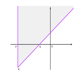
Figure 1: Configuration of $h\leq g<0$

In the case of $h\leq 0\leq g$, $R$ is below the $u$-axis, $P$ is on the left side of $Q$, and $O$ is located in between $P$ and $Q$. As can be seen from Figure 2, the boundary can be expressed as

$$\mathscr{B}=\left\{\left(\frac{h}{\cos\phi},\phi\right):\frac{\pi}{2}<\phi\leq\pi+\phi_{R}\right\}\bigcup\left\{\left(\frac{g}{\sqrt{1+k^{2}}\cos(\phi+\phi_{k})},\phi\right):\pi+\phi_{R}\leq\phi<2\pi+\frac{\pi}{2}-\phi_{k}\right\}.$$

By Theorem 5 and making use of a change of variable in the integration, we have $\Pr\{h\leq U\leq kV+g\}=1-\int^{\pi+\phi_{R}}_{\pi/2}\Psi_{h}(\phi)\;d\phi-\int^{3\pi/2}_{\phi_{k}+\phi_{R}}\Psi_{g,k}(\phi)\;d\phi$.

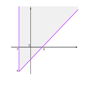
Figure 2: Configuration of $h\leq 0\leq g$

In the case of $0<h\leq g$, $O$ is on the left side of $P$, $P$ is on the left side of $Q$, and $R$ is below the $u$-axis. As can be seen from Figure 3, the visible and invisible parts of the boundary can be expressed as $\mathscr{B}_{\mathrm{v}}=\left\{\left(\frac{h}{\cos\phi},\phi\right):\phi_{R}\leq\phi<\frac{\pi}{2}\right\}$ and $\mathscr{B}_{\mathrm{i}}=\left\{\left(\frac{g}{\sqrt{1+k^{2}}\cos(\phi+\phi_{k})},\phi\right):\phi_{R}<\phi<\frac{\pi}{2}-\phi_{k}\right\}$ respectively. By Theorem 6 and making use of a change of variable in the integration, we have $\Pr\{h\leq U\leq kV+g\}=\int^{\pi/2}_{\phi_{R}}\Psi_{h}(\phi)\;d\phi-\int^{\pi/2}_{\phi_{k}+\phi_{R}}\Psi_{g,k}(\phi)\;d\phi$.

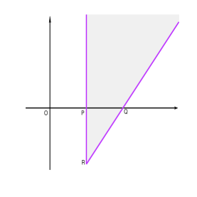
Figure 3: Configuration of $0<h\leq g$

In the case of $0<g<h$, $R$ is above the $u$-axis, $Q$ is on the left side of $P$, and $O$ is on the left side of $Q$. As can be seen from Figure 4, the visible and invisible parts of the boundary can be expressed as $\mathscr{B}_{\mathrm{v}}=\left\{\left(\frac{h}{\cos\phi},\phi\right):\phi_{R}\leq\phi<\frac{\pi}{2}\right\}$ and $\mathscr{B}_{\mathrm{i}}=\left\{\left(\frac{g}{\sqrt{1+k^{2}}\cos(\phi+\phi_{k})},\phi\right):\phi_{R}<\phi<\frac{\pi}{2}-\phi_{k}\right\}$ respectively. By Theorem 6 and making use of a change of variable in the integration, we have $\Pr\{h\leq U\leq kV+g\}=\int^{\pi/2}_{\phi_{R}}\Psi_{h}(\phi)\;d\phi-\int^{\pi/2}_{\phi_{k}+\phi_{R}}\Psi_{g,k}(\phi)\;d\phi$.

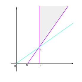
Figure 4: Configuration of $0<g<h$

In the case of $g\leq 0\leq h$, $R$ is above the $u$-axis, $Q$ is on the left side of $P$, and $O$ is located in between $Q$ and $P$. As can be seen from Figure 5, the boundary is completely visible and can be expressed as $\mathscr{B}_{\mathrm{v}}=\left\{\left(\frac{h}{\cos\phi},\phi\right):\phi_{R}\leq\phi<\frac{\pi}{2}\right\}\bigcup\left\{\left(\frac{g}{\sqrt{1+k^{2}}\cos(\phi+\phi_{k})},\phi\right):\frac{\pi}{2}-\phi_{k}<\phi<\phi_{R}\right\}$. By Theorem 6 and making use of a change of variable in the integration, we have $\Pr\{h\leq U\leq kV+g\}=\int^{\pi/2}_{\phi_{R}}\Psi_{h}(\phi)\;d\phi-\int^{\pi/2}_{\phi_{k}+\phi_{R}}\Psi_{g,k}(\phi)\;d\phi$.

Figure 5: Configuration of $g\leq 0\leq h$

In the case of $g<h<0$, $R$ is above the $u$-axis, $Q$ is on the left side of $P$, and $P$ is on the left side of $O$. As can be seen from Figure 6, the visible and invisible parts of the boundary can be expressed, respectively, as $\mathscr{B}_{\mathrm{v}}=\left\{\left(\frac{g}{\sqrt{1+k^{2}}\cos(\phi+\phi_{k})},\phi\right):\frac{\pi}{2}-\phi_{k}<\phi\leq\pi+\phi_{R}\right\}$ and $\mathscr{B}_{\mathrm{i}}=\left\{\left(\frac{h}{\cos\phi},\phi\right):\frac{\pi}{2}<\phi<\pi+\phi_{R}\right\}$. By Theorem 6 and making use of a change of variable in the integration, we have $\Pr\{h\leq U\leq kV+g\}=\int^{\pi+\phi_{k}+\phi_{R}}_{\pi/2}\Psi_{g,k}(\phi)\;d\phi-\int^{\pi+\phi_{R}}_{\pi/2}\Psi_{h}(\phi)\;d\phi$. This concludes the proof of the theorem.

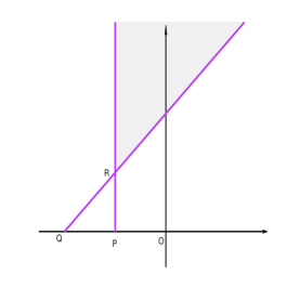
Figure 6: Configuration of $g<h<0$

Appendix F Proof of Theorem 8

We shall take a geometrical approach to prove Theorem 8. Before proceeding to the details of proof, we shall introduce some notations. For two points $P_{1},\;P_{2}$ on the $u$-axis, when $P_{1}$ is on the left side of $P_{2}$, we write $P_{1}<P_{2}$. Similarly, when $P_{1}$ is on the right side of $P_{2}$, we write $P_{1}>P_{2}$. We use $\widehat{P_{1}P_{2}}$ to denote the hyperbolic arc with end points $P_{1}$ and $P_{2}$. We define some special points $O=(0,0),\;A=(u_{A},v_{A}),\;B=(u_{B},v_{B}),\;C=(\vartheta+\sqrt{h},0),\;D=(\vartheta-\sqrt{h},0)$ and $M=(\vartheta,0)$ that will be frequently referred in the proof. The domain $\mathscr{D}$ is shaded for all configurations. The proof of Theorem 8 can be accomplished by showing Lemmas 2 to 9 in the sequel.

Lemma 2

For $\Pr\{(U,V)\in\mathscr{D}\}$ to be non-zero, $\vartheta,\lambda,g,h,k$ must satisfy one of the following four conditions: (i) $k^{2}<\lambda,\;g>\sqrt{h},\;\varDelta\geq 0$; (ii) $k^{2}<\lambda,\;0<g\leq\sqrt{h},\;\varDelta\geq 0$; (iii) $k^{2}>\lambda,\;gk>\sqrt{\varDelta}$; (iv) $k^{2}>\lambda,\;gk\leq\sqrt{\varDelta}$.

Proof.

Clearly, for $\Pr\{(U,V)\in\mathscr{D}\}$ to be non-zero, a necessary condition is that there exists at least one tuple $(u,v)$ satisfying equations $\sqrt{\lambda v^{2}+h}=u-\vartheta=kv+g$. By letting $z=u-\vartheta$, we can write the equations as $z-kv=g$ and $(k^{2}-\lambda)z^{2}+2\lambda g\;z-\lambda g^{2}-k^{2}h=0$ with $z\geq 0$, where the discriminant for the quadratic equation of $z$ is $4k^{2}\varDelta$. Therefore, the necessary condition for $\Pr\{(U,V)\in\mathscr{D}\}$ to be non-zero can be divided as two conditions: (I) $\varDelta\geq 0,\;g\geq 0,\;k^{2}<\lambda$; (II) $k^{2}>\lambda$.

If condition (I) holds, then the quadratic equation of $z$ have two non-negative roots: $z_{A}=\frac{\lambda g-k\sqrt{\varDelta}}{\lambda-k^{2}},\;z_{B}=\frac{\lambda g+k\sqrt{\varDelta}}{\lambda-k^{2}}$. Accordingly, there are two tuples $(u_{A},v_{A})$ and $(u_{B},v_{B})$ satisfying equations $\sqrt{\lambda v^{2}+h}=u-\vartheta=kv+g$ with $u_{A}=z_{A}+\vartheta,\;v_{A}=\frac{z_{A}-g}{k},\;u_{B}=z_{B}+\vartheta,\;v_{B}=\frac{z_{B}-g}{k}$. Noting that $v_{A},\;v_{B}$ are the roots for equation $(k^{2}-\lambda)v^{2}+2kgv+g^{2}-h=0$ with respect to $v$, condition (I) can be divided into conditions (i) and (ii) of the lemma such that (i) implies $\sqrt{h}+\vartheta<u_{A}<u_{B},\;v_{A}<0<v_{b}$ and that (ii) implies $\sqrt{h}+\vartheta<u_{A}<u_{B},\;0\leq v_{A}<v_{B}$.

If condition (II) holds, then the quadratic equation of $z$ have two roots $z_{A}$ and $z_{B}$ of opposite signs. Observing that $z_{A}>z_{B}$, we have $z_{A}=\frac{\lambda g-k\sqrt{\varDelta}}{\lambda-k^{2}}>0>z_{B}$. Since $v_{A}=\frac{z_{A}-g}{k}=\frac{gk-\sqrt{\varDelta}}{\lambda-k^{2}}\geq 0$ if and only if $gk\leq\sqrt{\varDelta}$, condition (II) can be divided into conditions (iii) and (iv) of the lemma such that (iii) implies $\sqrt{h}+\vartheta<u_{A},\;v_{A}<0$ and that (iv) implies $\sqrt{h}+\vartheta<u_{A},\;v_{A}\geq 0$. This completes the proof of the lemma.

$\Box$

Now we attempt to express the right branch hyperbola, $\mathscr{H}_{R}=\{(u,v):\sqrt{\lambda v^{2}+h}\leq u-\vartheta\}$ in polar coordinates $(r,\phi)$, which is related to the Cartesian coordinates by $u=r\cos\phi,\;v=r\sin\phi$. Note that the polar coordinates, $(r,\phi)$, of any point of $\mathscr{H}_{R}$ must satisfy the equation $(r\cos\phi-\vartheta)^{2}-\lambda(r\sin\phi)^{2}=h$ with respect to $r\geq 0$, which can be written as $(\cos^{2}\phi-\lambda\sin^{2}\phi)r^{2}-2\vartheta\cos\phi\;r+\eta=0$ with $\eta=\vartheta^{2}-h$. For $\phi$ such that $(h-\lambda\eta)\cos^{2}\phi+\lambda\eta\geq 0$, we have two real roots

$$r_{\diamond}(\phi)=\frac{\eta}{\vartheta\cos\phi+\sqrt{(h-\lambda\eta)\cos^{2}\phi+\lambda\eta}},\quad r_{\star}(\phi)=\frac{\eta}{\vartheta\cos\phi-\sqrt{(h-\lambda\eta)\cos^{2}\phi+\lambda\eta}}=-r_{\diamond}(\phi+\pi).$$

These are possible expressions for the relationship of polar coordinates $r$ and $\phi$ of the right branch hyperbola $\mathscr{H}_{R}$. However, it is not clear which expression should be taken. The specific expression and the visibility of $\mathscr{H}_{R}$ are to be determined in the sequel.

Lemma 3

If $O\leq M$, then the right hyperbola $\mathscr{H}_{R}$ is visible and can be expressed as $\mathscr{B}_{\mathrm{v}}=\{({r_{\star}},\phi):|\phi|<\phi_{\lambda}\}$.

Proof.

To show the lemma, we first need to show that ${r_{\star}}>0>{r_{\diamond}}$ for $1-\lambda\tan^{2}\phi>0$ and $D<O\leq M$. For $D<O\leq M$, we have $\vartheta-\sqrt{h}<0\leq\vartheta\Rightarrow\eta=\vartheta^{2}-h<0$. Thus, ${r_{\diamond}}<0$ as a result of $1-\lambda\tan^{2}\phi>0\Longleftrightarrow|\phi|<\phi_{\lambda}<\frac{\pi}{2}$. On the other hand, ${r_{\star}}=\frac{-\eta}{-\vartheta\cos\phi+\sqrt{(h-\lambda\eta)\cos^{2}\phi+\lambda\eta}}$. Observing that $(\vartheta\cos\phi)^{2}-\left[(h-\lambda\eta)\cos^{2}\phi+\lambda\eta\right]=\eta\cos^{2}\phi\;(1-\lambda\tan^{2}\phi)<0$ as a consequence of $\eta<0$ and $1-\lambda\tan^{2}\phi>0$, we have ${r_{\star}}>0$.

Next, we need to show that ${r_{\star}}>{r_{\diamond}}\geq 0$ for $1-\lambda\tan^{2}\phi>0$ and $O\leq D$. For $O\leq D$, we have $\vartheta-\sqrt{h}\geq 0\Rightarrow\eta=\vartheta^{2}-h\geq 0$. Thus, ${r_{\diamond}}\geq 0$. On the other hand, observing that $(\vartheta\cos\phi)^{2}-\left[(h-\lambda\eta)\cos^{2}\phi+\lambda\eta\right]=\eta\cos^{2}\phi\;(1-\lambda\tan^{2}\phi)\geq 0$ as a consequence of $\eta\geq 0$ and $1-\lambda\tan^{2}\phi>0$, we have ${r_{\star}}\geq 0$. Since the denominator of $r_{\star}$ is smaller than that of $r_{\diamond}$, we have ${r_{\star}}>{r_{\diamond}}\geq 0$. This completes the proof of the lemma.

$\Box$

Lemma 4

If $M<O\leq C$, then $\mathscr{B}_{\mathrm{v}}=\{({r_{\star}},\phi):|\phi|\leq\phi_{\mathrm{m}}\}$ and $\mathscr{B}_{\mathrm{i}}=\{({r_{\diamond}},\phi):\phi_{\lambda}<|\phi|<\phi_{\mathrm{m}}\}$.

Proof.

Since $M<O\leq C$, we have $\vartheta<0\leq\vartheta+\sqrt{h}\Rightarrow\eta=\vartheta^{2}-h\leq 0$. Hence, $(h-\lambda\eta)\cos^{2}\phi+\lambda\eta=h\cos^{2}\phi+\lambda\eta\sin^{2}\phi=-\lambda\eta\cos^{2}\phi\left(-\frac{h}{\lambda\eta}-\tan^{2}\phi\right)$, which implies that $(h-\lambda\eta)\cos^{2}\phi+\lambda\eta$ is nonnegative for $|\phi|\leq\phi_{\mathrm{m}}$ and negative for $\phi_{\mathrm{m}}<|\phi|<\frac{\pi}{2}$.

To show the lemma, we first need to show that ${r_{\star}}\geq 0\geq{r_{\diamond}}$ if $1-\lambda\tan^{2}\phi>0$. Since $\eta\leq 0$ and $\vartheta<0$, we have ${r_{\star}}=\frac{-\eta}{-\vartheta\cos\phi+\sqrt{(h-\lambda\eta)\cos^{2}\phi+\lambda\eta}}\geq 0$ in view of $1-\lambda\tan^{2}\phi>0\Longleftrightarrow|\phi|<\phi_{\lambda}<\frac{\pi}{2}$. On the other hand, observing that ${r_{\diamond}}=\frac{-\eta}{-\vartheta\cos\phi-\sqrt{(h-\lambda\eta)\cos^{2}\phi+\lambda\eta}}$ and $(\vartheta\cos\phi)^{2}-\left[(h-\lambda\eta)\cos^{2}\phi+\lambda\eta\right]=\eta\cos^{2}\phi\;(1-\lambda\tan^{2}\phi)<0$ as a consequence of $\eta\leq 0$ and $1-\lambda\tan^{2}\phi>0$, we have ${r_{\diamond}}\leq 0$.

Next, we need to show that $0\leq{r_{\star}}\leq{r_{\diamond}}$ if $\phi_{\lambda}<|\phi|<\phi_{\mathrm{m}}$. By the same argument as above, we have ${r_{\star}}\geq 0$ because $|\phi|<\frac{\pi}{2}$. It remains to show ${r_{\star}}<{r_{\diamond}}$. Note that $(\vartheta\cos\phi)^{2}-\left[(h-\lambda\eta)\cos^{2}\phi+\lambda\eta\right]=\eta\cos^{2}\phi(1-\lambda\tan^{2}\phi)$ is positive as a result of $\eta\leq 0$ and $\phi_{\lambda}<|\phi|<\phi_{\mathrm{m}}\Rightarrow 1-\lambda\tan^{2}\phi<0$. Since $\vartheta\cos\phi<0$ as a consequence of $\vartheta<0$ and $\phi_{\lambda}<|\phi|<\phi_{\mathrm{m}}$, it follows that $-\vartheta\cos\phi-\sqrt{(h-\lambda\eta)\cos^{2}\phi+\lambda\eta}>0$ and thus ${r_{\diamond}}\geq 0$. Since the numerators of ${r_{\star}}$ and ${r_{\diamond}}$ are equal to the same non-negative number and the denominator of ${r_{\diamond}}$ is a positive number smaller than that of ${r_{\star}}$, we have ${r_{\diamond}}\geq{r_{\star}}\geq 0$. This completes the proof of the lemma. $\Box$

As can be seen from the proof of Lemma 4, the boundary is divided into visible part $\mathscr{B}_{\mathrm{v}}$ and invisible part $\mathscr{B}_{\mathrm{i}}$ by the upper critical point $\left(\frac{\eta}{\vartheta\cos\phi_{m}},\phi_{m}\right)$ and the lower critical point $\left(\frac{\eta}{\vartheta\cos\phi_{m}},-\phi_{m}\right)$. The visible part is on the left side of the critical line, which is referred to as the vertical line connecting the lower and upper critical points. The invisible part is on the right side of the critical line.

Lemma 5

If $O>C$, then the right hyperbola $\mathscr{H}_{R}$ can be represented as $\{({r_{\diamond}},\phi):\phi_{\lambda}<\phi<2\pi-\phi_{\lambda}\}$.

Proof.

To show the lemma, we first need to show that ${r_{\star}}<0<{r_{\diamond}}$ for $\phi_{\lambda}<\phi<\pi-\phi_{\lambda}$ and $\pi+\phi_{\lambda}<\phi<2\phi-\phi_{\lambda}$. Since $O>C$, we have $\vartheta<-\sqrt{h}$ and thus $\eta=\vartheta^{2}-h>0$. Since $1-\lambda\tan^{2}\phi<0$ for $\phi_{\lambda}<\phi<\pi-\phi_{\lambda}$ and $\pi+\phi_{\lambda}<\phi<2\pi-\phi_{\lambda}$, we have $|\vartheta\cos\phi|-\sqrt{(h-\lambda\eta)\cos^{2}\phi+\lambda\eta}<0$, leading to ${r_{\star}}<0$. On the other hand, $\vartheta\cos\phi+\sqrt{(h-\lambda\eta)\cos^{2}\phi+\lambda\eta}>-|\vartheta\cos\phi|+\sqrt{(h-\lambda\eta)\cos^{2}\phi+\lambda\eta}>0$, leading to ${r_{\diamond}}>0$.

Next, we need to show that ${r_{\star}}>{r_{\diamond}}>0$ for $\pi-\phi_{\lambda}<\phi<\pi+\phi_{\lambda}$. For $\pi-\phi_{\lambda}<\phi<\pi+\phi_{\lambda}$, we have $1-\lambda\tan^{2}\phi>0$. Since $\eta>0$ and $\vartheta<0$, it must be true that $\vartheta\cos\phi>0$ and ${r_{\diamond}}>0$. As a consequence of $\vartheta\cos\phi>0$ and $1-\lambda\tan^{2}\phi>0$, we have that the denominator of ${r_{\star}}$ is positive. Recalling that the numerator of ${r_{\star}}$ is a positive number $\eta$, we have ${r_{\star}}>0$. Since the numerators of ${r_{\star}}$ and ${r_{\diamond}}$ are equal to the same positive number $\eta$ and the denominator of ${r_{\star}}$ is a positive number smaller than that of ${r_{\diamond}}$, we have ${r_{\star}}>{r_{\diamond}}>0$. This completes the proof of the lemma.

$\Box$

Lemma 6

If $k^{2}<\lambda,\;g>\sqrt{h}$ and $\varDelta\geq 0$, then $\Pr\{(U,V)\in\mathscr{D}\}=I_{\mathrm{np}}$.

Proof.

As consequence of $k^{2}<\lambda,\;g>\sqrt{h}$ and $\varDelta\geq 0$, we have $\sqrt{h}+\vartheta<u_{A}<u_{B},\;v_{A}<0<v_{B}$. The tangent line at $A$ intercepts the $u$-axis at $P=(u_{P},0)$ with $u_{P}$ satisfying $\frac{\sqrt{(u_{A}-\vartheta)^{2}-h}}{\sqrt{\lambda}\;(u_{A}-u_{P})}=\frac{u_{A}-\vartheta}{\sqrt{\lambda}\sqrt{(u_{A}-\vartheta)^{2}-h}}$, from which we obtain $u_{P}=\vartheta+\frac{h}{u_{A}-\vartheta}>\vartheta$. Similarly, the tangent line at $B$ intercepts the $u$-axis at $Q=(u_{Q},0)$ with $u_{Q}=\vartheta+\frac{h}{u_{B}-\vartheta}<u_{P}<u_{C}$. Line $AB$ intercepts the $u$-axis at $R=(u_{R},0)$ with $u_{R}=g+\vartheta$. Clearly, $D<M<Q<P<C$. The lemma can be shown by investigating five cases as follows.

In the case of $\vartheta+\frac{h}{u_{B}-\vartheta}\geq 0$, we have $O\leq Q$. The situation is shown in Figure 7. If $O\leq M$, then, by Lemma 2, the right branch hyperbola $\mathscr{H}_{R}$ is completely visible. Accordingly, the visible and invisible parts of the boundary of $\mathscr{D}$ can be expressed, respectively, as $\mathscr{B}_{\mathrm{v}}=\{({r_{\star}},\phi):-\phi_{A}\leq\phi\leq\phi_{B}\}$ and $\mathscr{B}_{\mathrm{i}}=\{(r_{l},\phi):-\phi_{A}<\phi<\phi_{B}\}$, where $r_{l}(\phi)=\frac{g+\vartheta}{\sqrt{1+k^{2}}\cos(\phi+\phi_{k})}$. Now consider the situation that $M<O\leq Q$. Since the domain, $\mathscr{H}=\{(u,v):\sqrt{\lambda v^{2}+h}\leq u-\vartheta\}$, corresponding to the region included by the right branch hyperbola $\mathscr{H}_{R}$, is a convex set, we have that $\mathscr{H}$ is divided by line $OA$ into two sub-domains of which one is below line $OA$ and above the tangent line $PA$, and the other is above both line $OA$ and the tangent line $PA$. As can be seen from Figure 7, the lower critical point $\left(\frac{\eta}{\vartheta\cos\phi_{m}},-\phi_{m}\right)$ must be below line $OA$. It follows from Lemma 3 that arc $\widehat{AC}$ is visible. By a similar argument, we have that arc $\widehat{CB}$ is visible. Therefore, by Lemma 3, the visible and invisible parts of the boundary of $\mathscr{D}$ can be expressed, respectively, as $\mathscr{B}_{\mathrm{v}}$ and $\mathscr{B}_{\mathrm{i}}$ like the case of $O\leq M$. Applying Theorem 6 yields $\Pr\{(U,V)\in\mathscr{D}\}=I_{\mathrm{np},1}$.

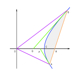
Figure 7: Configuration of $O\leq Q$

In the case of $\vartheta+\frac{h}{u_{B}-\vartheta}<0\leq\vartheta+\frac{h}{u_{A}-\vartheta}$, we have $Q<O\leq P$. The situation is shown in Figure 8. Recall that arc $\widehat{AC}$ is visible as in the preceding case of $O\leq Q$. Since the domain $\mathscr{H}$ is a convex set, we have that $\mathscr{H}$ is divided by line $OB$ into two sub-domains of which one is above line $OB$ and below the tangent line $QB$, and the other is below both line $OB$ and the tangent line $QB$. As can be seen from Figure 8, the upper critical point $\left(\frac{\eta}{\vartheta\cos\phi_{m}},\phi_{m}\right)$ must be above line $OB$. Hence, applying Lemma 3, the visible and invisible parts of the boundary of $\mathscr{D}$ can be expressed, respectively, as $\mathscr{B}_{\mathrm{v}}=\{({r_{\star}},\phi):-\phi_{A}\leq\phi\leq\phi_{\mathrm{m}}\}$ and $\mathscr{B}_{\mathrm{i}}=\{(r_{l},\phi):-\phi_{A}<\phi<\phi_{B}\}\cup\{({r_{\diamond}},\phi):\phi_{B}\leq\phi<\phi_{\mathrm{m}}\}$. Applying Theorem 6 yields $\Pr\{(U,V)\in\mathscr{D}\}=I_{\mathrm{np},2}$.

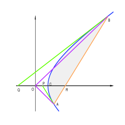
Figure 8: Configuration of $Q<O\leq P$

In the case of $\vartheta+\frac{h}{u_{A}-\vartheta}<0\leq\vartheta+\sqrt{h}$, we have $P<O\leq C$. The situation is shown in Figure 9. By a similar method as that of the case of $Q<O\leq P$, we have that the upper critical point must be above line $OB$ and in arc $\widehat{CB}$ and that the lower critical point must be below line $OA$ and in arc $\widehat{AC}$. Hence, by Lemma 3, the visible and invisible parts of the boundary of $\mathscr{D}$ can be expressed, respectively, as $\mathscr{B}_{\mathrm{v}}=\{({r_{\star}},\phi):-\phi_{\mathrm{m}}\leq\phi\leq\phi_{\mathrm{m}}\}$ and $\mathscr{B}_{\mathrm{i}}=\{(r_{l},\phi):-\phi_{A}\leq\phi\leq\phi_{B}\}\cup\{({r_{\diamond}},\phi):-\phi_{\mathrm{m}}<\phi<-\phi_{A}\}\cup\{({r_{\diamond}},\phi):\phi_{B}<\phi<\phi_{\mathrm{m}}\}$. By virtue of Theorem 6, we have $\Pr\{(U,V)\in\mathscr{D}\}=I_{\mathrm{np},3}$.

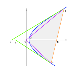
Figure 9: Configuration of $P<O\leq C$

In the case of $\vartheta+\sqrt{h}<0\leq g+\vartheta$, we have $C<O\leq R$. The situation is shown in Figure 10. By Lemma 4, the boundary of $\mathscr{D}$ can be expressed as $\mathscr{B}=\{(r_{l},\phi):-\phi_{A}\leq\phi\leq\phi_{B}\}\cup\{({r_{\diamond}},\phi):\phi_{B}<\phi<2\pi-\phi_{A}\}$. By virtue of Theorem 5, we have $\Pr\{(U,V)\in\mathscr{D}\}=I_{\mathrm{np},4}$.

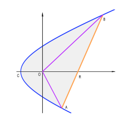
Figure 10: Configuration of $C<O\leq R$

In the case of $g+\vartheta<0$, we have $O>R$. The situation is shown in Figure 11. By Lemma 4, the visible and invisible parts of the boundary of $\mathscr{D}$ can be expressed, respectively, as $\mathscr{B}_{\mathrm{v}}=\{(r_{l},\phi):\phi_{B}\leq\phi\leq 2\pi-\phi_{A}\}$ and $\mathscr{B}_{\mathrm{i}}=\{({r_{\diamond}},\phi):\phi_{B}<\phi<2\pi-\phi_{A}\}$. By virtue of Theorem 6, we have $\Pr\{(U,V)\in\mathscr{D}\}=I_{\mathrm{np},5}$.

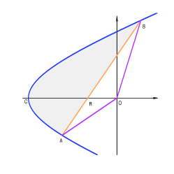
Figure 11: Configuration of $O>R$

$\Box$

Lemma 7

If $k^{2}<\lambda,\;0\leq g\leq\sqrt{h}$, then $\Pr\{(U,V)\in\mathscr{D}\}=I_{\mathrm{pp}}$.

Proof.

As a consequence of $k^{2}<\lambda,\;0\leq g\leq\sqrt{h}$ and $\varDelta\geq 0$, we have $\sqrt{h}+\vartheta<u_{A}<u_{B},\;0\leq v_{A}<v_{B}$. Clearly, $D<M<Q<R<P<C$. The lemma can be shown by investigating several cases as follows.

In the case of $\vartheta+\frac{h}{u_{B}-\vartheta}\geq 0$, we have $O\leq Q$. The situation is shown in Figure 12. By Lemmas 2 and 3, and a similar argument as that of the first case of Lemma 6, the visible and invisible parts of the boundary of $\mathscr{D}$ can be determined, respectively, as $\mathscr{B}_{\mathrm{v}}=\{({r_{\star}},\phi):\phi_{A}\leq\phi\leq\phi_{B}\}$ and $\mathscr{B}_{\mathrm{i}}=\{(r_{l},\phi):\phi_{A}<\phi<\phi_{B}\}$. By virtue of Theorem 6, we have $\Pr\{(U,V)\in\mathscr{D}\}=I_{\mathrm{pp},1}$.

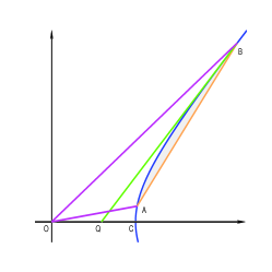
Figure 12: Configuration of $O\leq Q$

In the case of $\vartheta+\frac{h}{u_{B}-\vartheta}<0\leq g+\vartheta$, we have $Q<O\leq R$. The situation is shown in Figure 13. By Lemma 3 and a similar argument as that of the second case of Lemma 6, the visible and invisible parts of the boundary of $\mathscr{D}$ can be determined, respectively, as $\mathscr{B}_{\mathrm{v}}=\{({r_{\star}},\phi):\phi_{A}\leq\phi\leq\phi_{\mathrm{m}}\}$ and $\mathscr{B}_{\mathrm{i}}=\{(r_{l},\phi):\phi_{A}<\phi\leq\phi_{B}\}\cup\{({r_{\diamond}},\phi):\phi_{B}<\phi<\phi_{\mathrm{m}}\}$. By virtue of Theorem 6, we have $\Pr\{(U,V)\in\mathscr{D}\}=I_{\mathrm{pp},2}$.

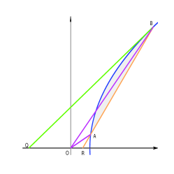
Figure 13: Configuration of $Q<O\leq R$

In the case of $g+\vartheta<0\leq\vartheta+\frac{h}{u_{A}-\vartheta}$, we have $R<O\leq P$. The situation is shown in Figure 14. Observing that the upper critical point must be above $OA$ and thus must be in arc $\widehat{AS}$, by Lemma 3, we have that the visible and invisible parts of the boundary of $\mathscr{D}$ can be expressed, respectively, as $\mathscr{B}_{\mathrm{v}}=\{({r_{\star}},\phi):\phi_{A}\leq\phi\leq\phi_{\mathrm{m}}\}\cup\{(r_{l},\phi):\phi_{B}\leq\phi<\phi_{A}\}$ and $\mathscr{B}_{\mathrm{i}}=\{({r_{\diamond}},\phi):\phi_{B}<\phi<\phi_{\mathrm{m}}\}$. By virtue of Theorem 6, we have $\Pr\{(U,V)\in\mathscr{D}\}=I_{\mathrm{pp},2}$.

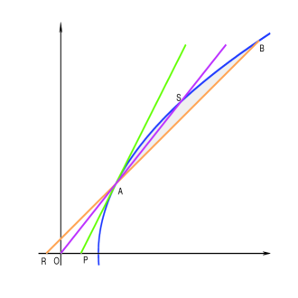
Figure 14: Configuration of $R<O\leq P$

In the case of $\vartheta+\frac{h}{u_{A}-\vartheta}<0\leq\vartheta+\sqrt{h}$, we have $P<O\leq C$. The situation is shown in Figure 15. Observing that the upper critical point must be in the part of arc $\widehat{CA}$ that is above $OA$, by Lemma 3, we have that the visible and invisible parts of the boundary of $\mathscr{D}$ can be determined, respectively, as $\mathscr{B}_{\mathrm{v}}=\{(r_{l},\phi):\phi_{B}\leq\phi\leq\phi_{A}\}$ and $\mathscr{B}_{\mathrm{i}}=\{({r_{\diamond}},\phi):\phi_{B}<\phi<\phi_{A}\}$. By virtue of Theorem 6, we have $\Pr\{(U,V)\in\mathscr{D}\}=I_{\mathrm{pp},3}$.

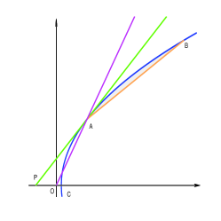
Figure 15: Configuration of $P<O\leq C$

In the case of $\vartheta+\sqrt{h}<0$, we have $O>C$. The situation is shown in Figure 16. By Lemma 4, the visible and invisible parts of the boundary of $\mathscr{D}$ can be determined, respectively, as $\mathscr{B}_{\mathrm{v}}=\{(r_{l},\phi):\phi_{B}\leq\phi\leq\phi_{A}\}$ and $\mathscr{B}_{\mathrm{i}}=\{({r_{\diamond}},\phi):\phi_{B}<\phi<\phi_{A}\}$. By virtue of Theorem 6, we have $\Pr\{(U,V)\in\mathscr{D}\}=I_{\mathrm{pp},3}$.

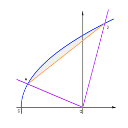
Figure 16: Configuration of $O>C$

$\Box$

Lemma 8

If $k^{2}>\lambda$ and $gk\leq\sqrt{\varDelta}$, then $\Pr\{(U,V)\in\mathscr{D}\}=I_{\mathrm{p}}$.

Proof.

Since $k^{2}>\lambda$ and $gk\leq\sqrt{\varDelta}$, we have $v_{A}\geq 0$. Consider straight line AB described by equation $u-\vartheta=kv+g$, passing through $A=(u_{A},v_{A})$. Suppose that the tangent line at $A$ intercepts the $u$-axis at $P$. Draw a line, denoted by $AF$, from $A$ with angle $\phi_{\lambda}$. Extend $FA$ to intercept the $u$-axis at $G$. Then, $u_{A}-u_{G}=\sqrt{\lambda}v_{A}$, leading to $u_{G}=u_{A}-\sqrt{\lambda}\;v_{A}$. The lemma can be shown by considering several cases as follows.

In the case of $\vartheta\geq 0$ and $\frac{v_{A}}{u_{A}}\geq\frac{1}{k}$, we have that $O\leq M$ and $AB$ is below $OA$. The situation is shown in Figure 17. Since $O\leq M$, by Lemma 2, the boundary of $\mathscr{D}$ is completely visible and can be expressed as $\mathscr{B}_{\mathrm{v}}=\{({r_{\star}},\phi):\phi_{A}\leq\phi<\phi_{\lambda}\}\cup\left\{(r_{l},\phi):\frac{\pi}{2}-\phi_{k}<\phi<\phi_{A}\right\}$. By virtue of Theorem 6, we have $\Pr\{(U,V)\in\mathscr{D}\}=I_{\mathrm{p},1}$.

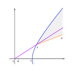
Figure 17: Configuration for $O\leq M$ and $AB$ below $OA$

In the case of $\vartheta\geq 0$ and $\frac{v_{A}}{u_{A}}<\frac{1}{k}$, we have that $O\leq M$ and $AB$ is above $OA$. The situation is shown in Figure 18. By Lemma 2, the visible and invisible parts of the boundary of $\mathscr{D}$ can be determined, respectively, as $\mathscr{B}_{\mathrm{v}}=\{({r_{\star}},\phi):\phi_{A}\leq\phi<\phi_{\lambda}\}$ and $\mathscr{B}_{\mathrm{i}}=\left\{(r_{l},\phi):\phi_{A}<\phi<\frac{\pi}{2}-\phi_{k}\right\}$. By virtue of Theorem 6, we have $\Pr\{(U,V)\in\mathscr{D}\}=I_{\mathrm{p},1}$.

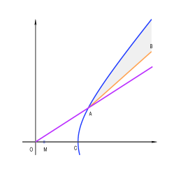
Figure 18: Configuration for $O\leq M$ and $AB$ above $OA$

In the case of $\vartheta<0\leq u_{A}-\sqrt{\lambda}\;v_{A}$ and $\frac{v_{A}}{u_{A}}\geq\frac{1}{k}$, we have that $M<O\leq G$ and $AB$ is below $OA$. The situation is shown in Figure 19. Making use of Lemma 3 and the observation that the upper critical point must be above $OA$, the visible and invisible parts of the boundary of $\mathscr{D}$ can be determined, respectively, as $\mathscr{B}_{\mathrm{v}}=\{({r_{\star}},\phi):\phi_{A}\leq\phi\leq\phi_{\mathrm{m}}\}\cup\left\{(r_{l},\phi):\frac{\pi}{2}-\phi_{k}<\phi<\phi_{A}\right\}$ and $\mathscr{B}_{\mathrm{i}}=\{({r_{\diamond}},\phi):\phi_{\lambda}<\phi<\phi_{\mathrm{m}}\}$. By virtue of Theorem 6, we have $\Pr\{(U,V)\in\mathscr{D}\}=I_{\mathrm{p},2}$.

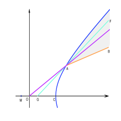
Figure 19: Configuration for $M<O\leq G$ and $AB$ below $OA$

In the case of $\vartheta<0\leq u_{A}-\sqrt{\lambda}\;v_{A}$ and $\frac{v_{A}}{u_{A}}<\frac{1}{k}$, we have that $M<O\leq G$ and $AB$ is above $OA$. The situation is shown in Figure 20. Since the upper critical point must be above $OA$, by Lemma 3, the visible and invisible parts of the boundary of $\mathscr{D}$ can be determined, respectively, as $\mathscr{B}_{\mathrm{v}}=\{({r_{\star}},\phi):\phi_{A}\leq\phi\leq\phi_{\mathrm{m}}\}$ and $\mathscr{B}_{\mathrm{i}}=\{({r_{\diamond}},\phi):\phi_{\lambda}<\phi<\phi_{\mathrm{m}}\}\cup\left\{(r_{l},\phi):\phi_{A}<\phi<\frac{\pi}{2}-\phi_{k}\right\}$. By virtue of Theorem 6, we have $\Pr\{(U,V)\in\mathscr{D}\}=I_{\mathrm{p},2}$.

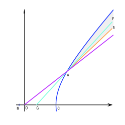
Figure 20: Configuration for $M<O\leq G$ and $AB$ above $OA$

In the case of $u_{A}-\sqrt{\lambda}\;v_{A}<0\leq\vartheta+\frac{h}{u_{A}-\vartheta}$, we have that $G<O\leq P$. The situation is shown in Figure 21. Since $k^{2}>\lambda$, the slope of line $AB$ is smaller than that of line $AF$. As a consequence of $G<O$, the slope of line $AF$ must be smaller than that of line $OA$. Hence, the slope of line $AB$ must be smaller than that of line $OA$. Making use of this observation and noting that the upper critical point must be above $OA$, we can apply Lemma 3 to determine the visible and invisible parts of the boundary of $\mathscr{D}$, respectively, as $\mathscr{B}_{\mathrm{v}}=\{({r_{\star}},\phi):\phi_{A}\leq\phi\leq\phi_{\mathrm{m}}\}\cup\left\{(r_{l},\phi):\frac{\pi}{2}-\phi_{k}<\phi<\phi_{A}\right\}$ and $\mathscr{B}_{\mathrm{i}}=\{({r_{\diamond}},\phi):\phi_{\lambda}<\phi<\phi_{\mathrm{m}}\}$. By virtue of Theorem 6, we have $\Pr\{(U,V)\in\mathscr{D}\}=I_{\mathrm{p},2}$.

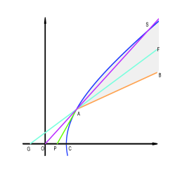
Figure 21: Configuration of $G<O\leq P$

In the case of $\vartheta+\frac{h}{u_{A}-\vartheta}<0\leq\vartheta+\sqrt{h}$, we have $P<O\leq C$. The situation is shown in Figure 22. Observing that the upper critical point must be in the part of arc $\widehat{CA}$ that is above line $OA$, by Lemma 3, the visible and invisible parts of the boundary of $\mathscr{D}$ can be determined, respectively, as $\mathscr{B}_{\mathrm{v}}=\left\{(r_{l},\phi):\frac{\pi}{2}-\phi_{k}<\phi\leq\phi_{A}\right\}$ and $\mathscr{B}_{\mathrm{i}}=\{({r_{\diamond}},\phi):\phi_{\lambda}<\phi<\phi_{A}\}$. By virtue of Theorem 6, we have $\Pr\{(U,V)\in\mathscr{D}\}=I_{\mathrm{p},3}$.

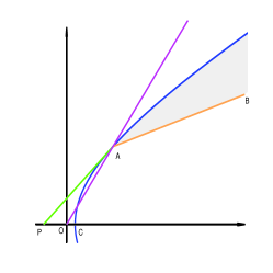
Figure 22: Configuration of $P<O\leq C$

In the case of $\vartheta+\sqrt{h}<0$, we have $C<O$. The situation is shown in Figure 23. By Lemma 4, the visible and invisible parts of the boundary of $\mathscr{D}$ can be expressed, respectively, as $\mathscr{B}_{\mathrm{v}}=\left\{(r_{l},\phi):\frac{\pi}{2}-\phi_{k}<\phi\leq\phi_{A}\right\}$ and $\mathscr{B}_{\mathrm{i}}=\{({r_{\diamond}},\phi):\phi_{\lambda}<\phi<\phi_{A}\}$. By virtue of Theorem 6, we have $\Pr\{(U,V)\in\mathscr{D}\}=I_{\mathrm{p},3}$.

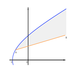
Figure 23: Configuration of $C<O$

$\Box$

Lemma 9

If $k^{2}>\lambda$ and $gk>\sqrt{\varDelta}$, then $\Pr\{(U,V)\in\mathscr{D}\}=I_{\mathrm{n}}$.

Proof.

For $k^{2}>\lambda$ and $gk>\sqrt{\varDelta}$. Then, $v_{A}<0$. The lemma can be shown by investigating five cases as follows.

In the case of $\vartheta\geq 0$, we have $O\leq M$. The situation is shown in Figure 24. Since $O\leq M$, by Lemma 2, the right branch hyperbola $\mathscr{H}_{R}$ is completely visible. Therefore, the visible and invisible parts of the boundary of $\mathscr{D}$ can be determined, respectively, as $\mathscr{B}_{\mathrm{v}}=\{({r_{\star}},\phi):-\phi_{A}\leq\phi<\phi_{\lambda}\}$ and $\mathscr{B}_{\mathrm{i}}=\left\{(r_{l},\phi):-\phi_{A}<\phi<\frac{\pi}{2}-\phi_{k}\right\}$. By virtue of Theorem 6, we have $\Pr\{(U,V)\in\mathscr{D}\}=I_{\mathrm{n},1}$.

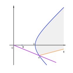
Figure 24: Configuration of $O\leq M$

In the case of $\vartheta<0\leq\vartheta+\frac{h}{u_{A}-\vartheta}$, we have $M<O\leq P$. The situation is shown in Figure 25. Observing that the lower critical point must be below line $OA$, by Lemma 3, we have that arc $\widehat{AC}$ must be visible and that the visible and invisible parts of the boundary of $\mathscr{D}$ can be determined, respectively, as $\mathscr{B}_{\mathrm{v}}=\{({r_{\star}},\phi):-\phi_{A}\leq\phi\leq\phi_{\mathrm{m}}\}$ and $\mathscr{B}_{\mathrm{i}}=\left\{(r_{l},\phi):-\phi_{A}<\phi<\frac{\pi}{2}-\phi_{k}\right\}\cup\{({r_{\diamond}},\phi):\phi_{\lambda}<\phi<\phi_{\mathrm{m}}\}$. By virtue of Theorem 6, we have $\Pr\{(U,V)\in\mathscr{D}\}=I_{\mathrm{n},2}$.

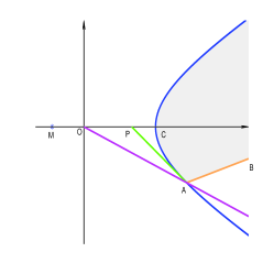
Figure 25: Configuration of $M<O\leq P$

In the case of $\vartheta+\frac{h}{u_{A}-\vartheta}<0\leq\vartheta+\sqrt{h}$, we have $P<O\leq C$. The situation is shown in Figure 26. Observing that the lower critical point must be in the part of arc $\widehat{AC}$ that is below line $OA$, by Lemma 3, we have that the visible and invisible parts of the boundary of $\mathscr{D}$ can be determined, respectively, as $\mathscr{B}_{\mathrm{v}}=\{({r_{\star}},\phi):-\phi_{\mathrm{m}}\leq\phi\leq\phi_{\mathrm{m}}\}$ and $\mathscr{B}_{\mathrm{i}}=\left\{(r_{l},\phi):-\phi_{A}<\phi<\frac{\pi}{2}-\phi_{k}\right\}\cup\{({r_{\diamond}},\phi):\phi_{\lambda}<\phi<\phi_{\mathrm{m}}\}\cup\{({r_{\diamond}},\phi):-\phi_{\mathrm{m}}<\phi\leq-\phi_{A}\}$. By virtue of Theorem 6, we have $\Pr\{(U,V)\in\mathscr{D}\}=I_{\mathrm{n},3}$.

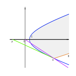
Figure 26: Configuration of $P<O\leq C$

In the case of $\vartheta+\sqrt{h}<0\leq\vartheta+g$, we have $C<O\leq R$. The situation is shown in Figure 27. By Lemma 4, the boundary of $\mathscr{D}$ can be expressed as $\mathscr{B}=\left\{(r_{l},\phi):-\phi_{A}\leq\phi\leq\frac{\pi}{2}-\phi_{k}\right\}\cup\{({r_{\diamond}},\phi):\phi_{\lambda}<\phi<2\pi-\phi_{A}\}$. By virtue of Theorem 5, we have $\Pr\{(U,V)\in\mathscr{D}\}=I_{\mathrm{n},4}$.

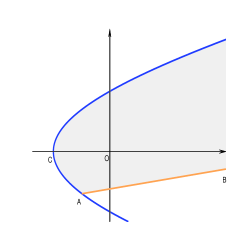
Figure 27: Configuration of $C<O\leq R$

In the case of $\vartheta+g<0$, we have $R<O$. The situation is shown in Figure 28. By Lemma 4, the visible and invisible parts of the boundary of $\mathscr{D}$ can be determined, respectively, as $\mathscr{B}_{\mathrm{v}}=\{(r_{l},\phi):\frac{\pi}{2}-\phi_{k}<\phi\leq 2\pi-\phi_{A}\}$ and $\mathscr{B}_{\mathrm{i}}=\{({r_{\diamond}},\phi):\phi_{\lambda}<\phi<2\pi-\phi_{A}\}$. By virtue of Theorem 6, we have $\Pr\{(U,V)\in\mathscr{D}\}=I_{\mathrm{n},5}$. This completes the proof of the theorem.

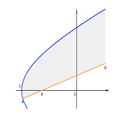
Figure 28: Configuration of $R<O$

$\Box$

References

- [1]
- [2] X. Chen, “A new framework of multistage estimation,” arXiv:0809.1241 [math.ST], September 2008.
- [3] X. Chen, “A new framework of multistage hypothesis tests,” arXiv:0809.3170 [math.ST], September 2008.
- [4] B. K. Ghosh and P. K. Sen (eds.), Handbook of Sequential Analysis, Dekker, New York, 1991.
- [5] A. Wald, Sequential Analysis, Wiley, New York, 1947.