Magnetism Localization in Spin-Polarized One-Dimensional Anderson–Hubbard Model

Abstract

In order to study an interplay of disorder, correlation, and spin imbalance on antiferromagnetism, we systematically explore the ground state of one-dimensional spin-imbalanced Anderson–Hubbard model by using the density-matrix renormalization group method. We find that disorders localize the antiferromagnetic spin density wave induced by imbalanced fermions and the increase of the disorder magnitude shrinks the areas of the localized antiferromagnetized regions. Moreover, the antiferromagnetism finally disappears above a large disorder. These behaviors are observable in atomic Fermi gases loaded on optical lattices and disordered strongly-correlated chains under magnetic field.

An atomic Fermi gas loaded on an optical lattice (FGOL) has been one of the most active target in the atomic gas field OLFermi since the successful observation of the superfluid-insulator transition in the Bose counterpart OLBose . In FGOL, its interaction tunability associated with the Feshbach resonance and lattice formation flexibility due to optical operations offer a great opportunity to systematically study the Hubbard model stripe and its extended versions Gao ; Okumura . Thus, FGOL is expected to be a promising experimental reality to resolve a wide range of controversial issues in condensed matter physics OLtheory .

The pairing mechanism in High-$T_{\rm c}$ superconductors has been one of the mostly debated issues for the latest two decades. The superconductivity emerges by doping holes via chemical substitutions on the Mott-insulator mother phase dopedMott . This drastically complicates theoretical studies because the pairing occurs on the strongly-correlated stage influenced by disorders. This fact stimulates systematic studies for the Anderson–Hubbard (AH) model Anderson ; Hubbard ; 1DAH ; 1DAHring . FGOL is an good experimental testbed to solve the complicated problem Gao ; Okumura .

In addition to such a practical motivation from the condensed matter side, FGOL inspires its own unique interests which lead to new frontiers. Its typical example is an arbitrary spin imbalance, which has been the most intensive target for a recent few years in atomic Fermi gases ImbalanceEx . Therefore, in this paper, we investigate the spin imbalance effects on the AH model. This will be one of the most fruitful target as well as the balanced case for the future FGOL experiments. Moreover, we point out that its weak imbalance case has a real counterpart, which corresponds to disordered strongly-correlated materials under magnetic field MottHeisenberg . Thus, we examine the model from the weak imbalance side.

The spin imbalance is believed to bring about a spatially inhomogeneous pairing like Fulde–Ferrel–Larkin–Ovchinikov state FFLO in attractive Hubbard model NumFF . This is a widely spread idea, while the imbalance effects have been very little investigated in the repulsive case. We therefore concentrate on antiferromagnetic phases characteristic to the repulsive Hubbard model and study how not only the imbalance but also the disorder magnitude affect the phases. In this paper, we focus on one-dimensional (1D) repulsive polarized AH model at the half-filling by using the density matrix renormalization group (DMRG) method White ; DMRGreview . The highlight in this paper is that disorders localize antiferromagnetic phases accompanied by a phase separation from the non-magnetized one and finally eliminate the antiferromagnetism in a strong disorder range. These results are directly observable in FGOL’s by using the atomic-density profile probe which is presently the most standard technique (for the experimental setup, see Ref. Okumura ).

The Hamiltonian of the 1D AH model is given by

$$H_{\rm AH}=-t\sum_{\langle i,j\rangle,\sigma}c^{\dagger}_{\sigma i}c^{\phantom{{\dagger}}}_{\sigma j}+\sum_{i,\sigma}\epsilon_{i}n_{\sigma i}+\sum_{i}Un_{\uparrow i}n_{\downarrow i}\,,$$ (1)

where $\langle i,j\rangle$ refers to the nearest neighbors $i$ and $j=i\pm 1$, $t$ is the hopping parameter between the nearest neighbor lattice sites, $U$ is the on-site repulsion, $c^{\phantom{{\dagger}}}_{\sigma i}$ ($c_{\sigma i}^{\dagger}$) is the annihilation- (creation-) operator and $n_{\sigma i}(\equiv c^{\dagger}_{\sigma i}c^{\phantom{{\dagger}}}_{\sigma i})$ is the site density operator with spin index $\sigma=\uparrow,\downarrow$, and the random on-site potential $\epsilon_{i}$ is chosen by a box probability distribution ${\cal P}(\epsilon_{i})=\theta(W/2-|\epsilon_{i}|)/W$, where $\theta(x)$ is the step function and the parameter $W$ the disorder strength magnitude. In DMRG calculations, the number of states kept ($m$) is $500$–$700$ and these numbers ($m\geq 500$) are enough for the most cases. In the calculations, we apply the open boundary condition except for the comparison with the periodical condition and measure the site matter and spin density of fermions as $n_{\uparrow i}\pm n_{\downarrow i}$.

Let us show DMRG calculation results on the spin imbalanced AH model (1). Figure 1 displays a randomness amplitude ($W/t$) dependence of the on-site matter and spin density profile for the number of the total sites $L=100$, the number of the spin-up and spin-down fermions $(N_{\uparrow},N_{\downarrow})=(51,49)$ (half-filling), and $U/t=10$. In this case, two up-spin fermions do not have their (down-spin) partners. The matter density profile is almost flat for $W\leq U$ as seen in Figs. 1(a)–1(c), while it is drastically disturbed for $W\geq U$. This is completely the same as that of the well-known balanced case. However, the spin density profile is significantly different. Firstly, in the clean case as shown in Fig. 1(a) ($W/t=0$), one finds an antiferromagnetic spin density wave (ASDW) whose periodicity is found to be inversely proportional to $N_{\uparrow}-N_{\downarrow}$ [e.g., see Figs. 3(h) and 3(i), in which $N_{\uparrow}-N_{\downarrow}=2$ and $4$, respectively]. Here, it is noted that any ASDW phases are never observed in the perfectly balanced cases irrespective of the presence of randomness note1 . This clearly indicates that the imbalance is responsible for the ASDW phase. Secondly, as one increases the disorder strength, a part of the ASDW (amplitude) “locally” vanishes and the depressed regions expand as seen in Figs. 1(b) and 1(c). This tendency becomes remarkable when $W$ exceeds over $U$ as seen in Figs. 1(d) and 1(e), in which two ASDW phases are localized and isolated each other. This isolation can be explained by the complete localization of two excess up-spin fermions for $W>U$ since the ASDW can be created only at the localized spots of the excess up-spin particles. In fact, the change in the up and down spin profiles in Fig. 1(c)–1(e) supports the idea. The further increase of $W$ diminishes the antiferromagnetic structure as seen in Fig. 1(f), in which the localized structure is characterized by positive peaks instead of the staggered (plus-minus) moment alternation. This is because the strong randomness fully dominates over the other effects. However, we note here that it is difficult in this large disorder range to judge whether the result [Fig. 1(f)] is the true ground-state or not. The reason is that in this strong $W$ range tiny changes of $W$ (e.g., $W+\delta W$) give entirely different spin-density distributions in non-continuous manner, which is not observed when $0<W/t\leq 14$. Generally, it is well-known in strongly glassy situations that a tiny change in calculation parameters results in a drastic different consequence. Thus, we expect that there are a lot of local minima in this strong disorder range. Fig. 1(f) is a localization profile selected among those minima.

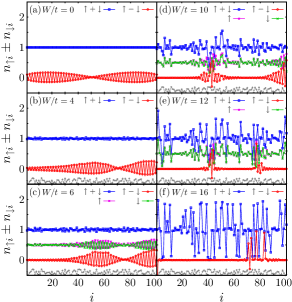
Figure 1: The randomness magnitude $W$ dependence of the matter and spin density profiles ($n_{\uparrow i}\pm n_{\downarrow i}$ respectively) at the half-filling for $U/t=10$ with $(N_{\uparrow},N_{\downarrow})=(51,49)$. A profile of the selected random potential is depicted on the bottom of each figure in an arbitrary unit (grey dashed line). In figures (c)–(e), up and down spin density profiles are shown. For all calculations, $m$ is 500.

In order to characterize the spin density profile in a wide range of $U$ and $W$, we define the following function,

$$S(U,W)=\left\langle\sum_{i=1}^{L}\frac{\left|n_{\uparrow i}(\epsilon,U,W)-n_{\downarrow i}(\epsilon,U,W)\right|}{L}\right\rangle_{\epsilon},$$ (2)

where $n_{\sigma i}(\epsilon,U,W)$ is the local site density under a random potential symbolically specified by $\epsilon$ at a certain set of $U$ and $W$, and $\langle\cdot\rangle_{\epsilon}$ means an algebraic average for various random realizations. From the expression, it is found that $S(U,W)$ gives an indicator how large the spin moment develops on each site. If the staggered moment widely grows, then $S(U,W)$ gives a relatively large value. Thus, a map of $S(U,W)$ in a wide range of $U$ and $W$ is expected to clarify an interplay of $U$ and $W$ on the ASDW phase localization. Figure 2(a) shows a contour plot of $S(U,W)$, which is averaged over ten realizations of random potentials for $L=100$ and $(N_{\uparrow},N_{\downarrow})=(51,49)$. In this figure, when one increases $W$ along a fixed $U/t$ line (e.g., $U/t=10$ line) from $W/t=0$ to $20$, it is found that the averaged moment of ASDW very slowly decreases inside the region $W<U$. This is consistent with the spin density profile as seen in Figs. 1(a)–1(c) in which the areas of ASDW phases slowly diminish with increasing $W$. When $W$ exceeds over $U$, the variation of $S(U,W)$ suddenly changes to a fast suppression. This reflects the change in the localization of the excess up-spin particles as seen in Figs. 1(c) and 1(d).

In order to qualify the present randomness averaging on Fig. 2(a), we introduce the following function

$$D(U,W)=\sqrt{\left\langle\left\{[S_{\epsilon}(U,W)/S(U,W)]-1\right\}^{2}\right\rangle_{\epsilon}}\,.$$ (3)

This corresponds to a standard deviation on the randomness average. Fig. 2(b) is a contour map of $D(U,W)$ in the same range as Fig. 2(a). One finds that in a small $W/t$ range $D(U,W)$ shows a very small value (almost zero) and $D(U,W)$ reaches about $0.2$ around $W=U+3t\sim 4t$ line when increasing $W/t$ at a constant $U/t$. Thus, the averaged values in Fig. 2(a) are sufficiently qualified except for above $W=U+3t$ line. This result means that the qualitative change as observed around $W=U$ in Fig. 2(a) is not a side effect associated with the averaging but an essential feature in this system.

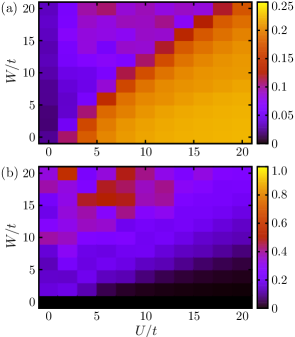
Figure 2: Contour plots of the value of (a) $S(U,W)$ [Eq. (2)] and (b) $D(U,W)$ [Eq. (3)] with $L=100$ and $(N_{\uparrow},N_{\downarrow})=(101,99)$ at the half-filling in a range of $U$ $(0\leq U\leq 20)$ and $W$ $(0\leq W\leq 20)$. The step value for both $U/t$ and $W/t$ is 2. For all calculations, $m$ is 500.

Next, we investigate the polarization strength dependence of the spin density profile. Figures 3(a)–3(g) display the correspondent results made at the half-filling in $L=200$, $U/t=18$ and $W/t=20$. In the range of these parameters, clear localization of the ASDW phases can be observed with the phase separation from the non-magnetized phases in a slight polarized case [e.g., see Fig. 1(d)]. Firstly, Fig. 3(a) displays the charge and spin density distributions in $(N_{\uparrow},N_{\downarrow})=(101,99)$. One finds two magnetized regions, in ASDW phases are localized with the localization of two extra fermions. The slight increase of the polarization [$(N_{\uparrow},N_{\downarrow})=(102,98)$] increases the number of the magnetized regions as seen in Fig. 3(b). Here, we note that the magnetized regions formed in the less polarized case as Fig. 3(a) are kept. This is in contrast to the clean systems ($W/t=0$) as shown in Figs. 3(h) and 3(i) whose polarizations are the same as Figs. 3(a) and 3(b), respectively. This is a typical feature characteristic to disordered systems, in which memory effects can be frequently observed. The further increase of the polarization extends the magnetized regions as shown in Figs. 3(c)–3(g). In Fig. 3(g), the magnetized (ASDW) regions cover all sites, which are almost positively polarized although the alternation profile still remains.

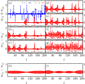
Figure 3: The polarization dependence of the spin density profiles [(a)–(g)] with $U/t=W/t=20$ and that without random potential [(h) and (i)] at $U/t=20$. The last two figures (h) and (i) without the randomness are displayed for a comparison with disordered cases (a) and (b) respectively. The number of up and down spin particles $(N_{\uparrow},N_{\downarrow})$ are (a) $(101,99)$, (b) $(102,98)$, (c) $(103,97)$, (d) $(104,96)$, (e) $(105,95)$, (f) $(110,90)$, (g) $(120,80)$, (h) $(101,99)$, and (i) $(102,98)$, respectively. The random potential shape are displayed on the bottom of the figures (a)–(g) (gray dashed lines). For all calculations, $m$ is 600.

We investigate a system size dependence of this magnetism localization to confirm that it is not a small size effect. In Figures 4(a)–4(c), we show the charge and spin density distributions at $U/t=W/t=20$ in $L=100$, $200$, and $300$ with $(N_{\uparrow},N_{\downarrow})=(51,49)$, $(102,98)$, and $(153,147)$, respectively. We clearly find that these all cases exhibit the same qualitative behavior, i.e., the magnetized regions are localized with the separation from the non-magnetized regions. From these figures, we find that the observed magnetism localization is an intrinsic effect.

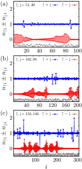
Figure 4: The size dependence of the matter and spin density profiles. The same polarization ratio is kept. (a) $L=100$ case with $(N_{\uparrow},N_{\downarrow})=(51,49)$, (b) $L=200$ case with $(N_{\uparrow},N_{\downarrow})=(102,98)$, and (c) $L=300$ case with $(N_{\uparrow},N_{\downarrow})=(153,147)$, respectively. $U/t=W/t=20$ in all cases. The random potential profiles are shown on the bottom of each figure (grey dashed lines). For all calculations, $m$ is 600.

Finally, we re-examine the model (1) under the periodic boundary condition to check the effect of the boundary condition. Figures 5(a)–5(f) show the $W$ dependent charge and spin density profiles in the periodic condition. In Fig. 5(a) ($W/t=0$), we find complete flat distributions in both the charge and spin densities. They are characteristic to the periodic boundary condition in which the excess fermions fully distribute homogeneously. This is in contrast to the open boundary condition [compare it with Fig. 1(a)]. When the randomness is added into the system, the ASDW phases are induced as seen in Figs. 5(b) and 5(c). Thus, one finds that the ASDW phase requires two conditions, i.e., the imbalance and the translational symmetry breaking. When the randomness strength increases, one finds that the amplitude of the ASDW increases [see Figs. 5(b) and 5(c)]. This implies that the localization of extra two fermions proceeds with increasing $W/t$. At $W/t=12$ and $14$ [see Figs. 5(d) and 5(e) for $W>U$], we find the phase separation from the non-magnetized phases, which is the same as the open boundary case. Further increase of $W/t$ brings about more tight localization [Fig. 5(e)] and disappearance of the staggered moment profile [Fig. 5(f)]. This is also the same as the open boundary case.

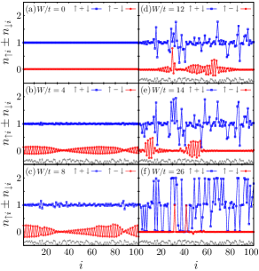
Figure 5: The randomness $W$ dependent matter and spin density profiles ($n_{\uparrow i}\pm n_{\downarrow i}$ respectively) with $L=100$, $(N_{\uparrow},N_{\downarrow})=(51,49)$, and $U/t=10$, under a random potential depicted on the bottom of each figure in arbitrary unit (grey dashed line). The periodic boundary condition is employed. For all calculations, $m$ is 700.

In conclusion, we systematically studied the polarized AH model at the half-filling and found that the disorder localizes the ASDW phases induced by the excess fermions. As the randomness strength increases, the areas of the localized ASDW phases shrink with the expansion of the non-magnetized areas, and the antiferromagnetism finally vanishes. These novel disorder effects on polarized strongly-correlated systems are observable in not only 1D FGOL’s Okumura but also strongly-correlated disordered chains under the magnetic field.

The authors wish to thank H. Aoki, T. Deguchi, K. Iida, T. Koyama, H. Matusmoto, Y. Ohashi, T. Oka, S. Tsuchiya, and Y. Yanase for illuminating discussion. The work was partially supported by Grant-in-Aid for Scientific Research (Grant No. 18500033) and one on Priority Area “Physics of new quantum phases in superclean materials” (Grant No. 18043022) from MEXT, Japan.

References

- (1) For the latest advancement, see, e.g., U. Schneider et al., arXiv:0809.1464.
- (2) M. Greiner et al., Nature 415, 39 (2002).
- (3) M. Machida, M. Okumura, and S. Yamada, Phys. Rev. A 77, 033619 (2008).
- (4) X. Gao et al., Phys. Rev. B 73, 161103 (2006); X. Gao, ibid 78, 085108 (2008).
- (5) M. Okumura et al., Phys. Rev. Lett. 101, 016407 (2008).
- (6) For a review, see, e.g., M. Lewenstein et al., Adv. Phys. 56, 243 (2007), and references therein.
- (7) See for a review, P.A. Lee, N. Nagaosa, and X.-G. Wen, Rev. Mod. Phys. 78, 17 (2006), and references therein.
- (8) P.W. Anderson, Phys. Rev. 109, 1492 (1958).
- (9) J. Hubbard, Proc. R. Soc. London, Ser. A 240, 539 (1957); ibid 243, 336 (1958).
- (10) M. Ma, Phys. Rev. B 26, 5097 (1982); A.W. Sandvik, D.J. Scalapino, and P. Henelius, ibid 50, 10474 (1994); R.V. Pai, A. Punnoose, and R.A. Römer, cond-mat/9704027; Y. Otsuka, Y. Morita, and Y. Hatsugai, Phys. Rev. B 58, 15314 (1998).
- (11) Another context is the persistent current in mesoscopic rings, which is not cited in this paper. For its recent progress, see, e.g., E. Gambetti, Phys. Rev. B 72, 165338 (2005), and references therein.
- (12) M.W. Zwierlein et al., Science 311, 492 (2006); G.B. Partridge et al., ibid 311, 503 (2006); M.W. Zwierlein et al., Nature 442, 54 (2006); Y. Shin et al., Phys. Rev. Lett. 97, 030401 (2006); G.B. Partridge et al., ibid 97, 190407 (2006); C.H. Schunck et al., Science 316, 867 (2007).
- (13) M. Machida et al., arXiv:0805.4261.
- (14) P. Fulde and R.A. Ferrell, Phys. Rev. 135, A550 (1964); A.I. Larkin and Y.N. Ovchinnikov, Zh. Eksp. Teor. Fiz. 47, 1136 (1964) [Sov. Phys. JETP, 20, 762 (1965)].
- (15) A.E. Feiguin and F. Heidrich-Meisner, Phys. Rev. B 76, 220508(R) (2007); M. Tezuka, and M. Ueda, Phys. Rev. Lett. 100, 110403 (2008); G.G. Batrouni et al., ibid 100, 116405 (2008); M. Rizzi et al., Phys. Rev. B 77, 245105 (2008); X. Gao and R. Asgari, Phys. Rev. A 77, 033604 (2008); M. Machida et al., ibid 77, 053614 (2008); A. Lüscher, R.M. Noack, and A.M. Läuchli, ibid 78, 013637 (2008); M. Casula, D.M. Ceperley, and E.J. Mueller, arXiv:0806.1747; A.E. Feiguin and F. Heidrich-Meisner, arXiv:0809.1539; A.E. Feiguin and D.A. Huse, arXiv:0809.3024.
- (16) S.R. White, Phys. Rev. Lett. 69, 2863 (1992); Phys. Rev. B 48, 10345 (1993).
- (17) For recent reviews, see e.g., U. Schollwöck, Rev. Mod. Phys. 77, 259 (2005); K.A. Hallberg, Adv. Phys. 55, 477 (2006), and references therein.
- (18) In this system, and are noted to be conserved respectively. They are also essentially conserved in FGOL.