Results of WEBT, VLBA and RXTE monitoring of 3C 279 during 2006–2007

Abstract

Context. The quasar 3C 279 is among the most extreme blazars in terms of luminosity and variability of flux at all wavebands. Its variations in flux and polarization are quite complex and therefore require intensive monitoring observations at multiple wavebands to characterise and interpret the observed changes.

Aims. In this paper, we present radio-to-optical data taken by the WEBT, supplemented by our VLBA and RXTE observations, of 3C 279. Our goal is to use this extensive database to draw inferences regarding the physics of the relativistic jet.

Methods. We assemble multifrequency light curves with data from 30 ground-based observatories and the space-based instruments SWIFT (UVOT) and RXTE, along with linear polarization vs. time in the optical $R$ band. In addition, we present a sequence of 22 images (with polarization vectors) at 43 GHz at resolution 0.15 milliarcsec, obtained with the VLBA. We analyse the light curves and polarization, as well as the spectral energy distributions at different epochs, corresponding to different brightness states.

Results. We find that the IR-optical-UV continuum spectrum of the variable component corresponds to a power law with a constant slope of $-1.6$, while in the 2.4–10 keV X-ray band it varies in slope from $-1.1$ to $-1.6$. The steepest X-ray spectrum occurs at a flux minimum. During a decline in flux from maximum in late 2006, the optical and 43 GHz core polarization vectors rotate by $\sim 300$°.

Conclusions. The continuum spectrum agrees with steady injection of relativistic electrons with a power-law energy distribution of slope $-3.2$ that is steepened to $-4.2$ at high energies by radiative losses. The X-ray emission at flux minimum comes most likely from a new component that starts in an upstream section of the jet where inverse Compton scattering of seed photons from outside the jet is important. The rotation of the polarization vector implies that the jet contains a helical magnetic field that extends $\sim 20$ pc past the 43 GHz core.

1 Introduction

Blazars form a class of active galactic nuclei in which the spectral energy distribution is dominated by highly variable nonthermal emission from relativistic jets that point almost directly along the line of sight. The quasar-type blazar 3C~279, at redshift $z=0.538$ (Burbidge & Rosenberg, 1965), is one of the most intensively studied objects of this class, owing to its pronounced variability of flux across the electromagnetic spectrum (by more than $5^{m}$ in optical bands) and high optical polarization (highest observed value of 45.5% in $U$ band, Mead et al. 1990). Because of this, 3C 279 has been the target of many multiwavelength campaigns, mounted in an effort to learn about the physics of the jet and the high-energy plasma that it contains. For example, in early 1996 the source was observed at a high $\gamma$-ray state, with extremely rapid flux variability, by the EGRET detector of the Compton Gamma Ray Observatory and at longer wavelengths near a historical maximum in brightness (Wehrle et al., 1998). The $\gamma$-ray flare was coincident with an X-ray outburst without any lag longer than 1 day. However, while one can draw some important conclusions from such campaigns, the behaviour of 3C 279 is typically too complex to characterise and relate conclusively to physical aspects of the jet from short-term light curves at a few wavelengths.

Ultra-high resolution observations with the Very Long Baseline Array (VLBA) have demonstrated that EGRET-detected blazars possess the most highly relativistic jets among compact flat spectrum radio sources (Jorstad et al., 2001a; Kellermann et al., 2004). This is inferred from the appearance of superluminally moving knots in the jet separating from a bright, compact, stationary “core” in the VLBA images. Apparent speeds in 3C 279 range from 4$c$ to 16$c$ (e.g., Jorstad et al., 2004, and references therein). From an analysis of both the apparent speeds and the time scales of flux decline of individual knots in 3C 279, Jorstad et al. (2005) derived a Doppler beaming factor $\delta=24\pm 6$, a Lorentz factor of the jet flow $\Gamma=16\pm 3$, and an angle between the jet axis and line of sight $\Theta\approx 2^{\circ}$. An analysis of the times of high $\gamma$-ray flux and superluminal ejections of $\gamma$-ray blazars indicates a statistical connection between the two events (Jorstad et al., 2001b). An intensive set of multi-waveband monitoring and VLBA observations of BL Lac confirms this connection between high-energy flares and superluminal knots in at least one blazar (Marscher et al., 2008).

Given the complexity of the time variability of nonthermal emission in blazars, a more complete observational dataset than customarily obtained is needed to maximize the range of conclusions that can be drawn concerning jet physics. To this end, Chatterjee et al. (2008) have analysed a decade-long dataset containing radio (14.5 GHz), single-colour ($R$-band) optical, and X-ray light curves as well as VLBA images at 43 GHz of 3C 279. They find strong correlations between the X-ray and optical fluxes, with time delays that change from X-ray leading optical variations to vice-versa, with simultaneous variations in between. Although the radio variations lag behind those in these wavebands by more than 100 days on average, changes in the jet direction on time scales of years are correlated with and actually lead long-term variations at X-ray energies. The current paper extends these observations to include multi-colour optical and near-infrared light curves, as well as linear polarization in the optical range and in the VLBA images, although over a more limited range in time (2006.0-2007.7). The radio-to-optical data presented in this paper have been acquired during a multifrequency campaign organized by the Whole Earth Blazar Telescope (WEBT) Our dataset includes the data from the 2006 WEBT campaign presented by Böttcher et al. (2007) as well as some of the data analysed by Chatterjee et al. (2008). The first of these papers found a spectral hardening during flares that appeared delayed with respect to a rising optical flux. The authors interpreted such behaviour in terms of inefficient particle acceleration at optical bands. Chatterjee et al. (2008) came to a similar conclusion based on the common occurrence of X-ray (from synchrotron self-Compton emission) variations leading optical synchrotron variations, with the latter involving higher-energy electrons than the former.

Our paper is organized as follows: Section 2 outlines the procedures that we used to process and analyse the data. Section 3 presents and analyses the multifrequency light curves, Sect. 4 discusses the kinematics and polarization of the radio jet as revealed by the VLBA images, and Sect. 5 gives the results of the optical polarimetry. In Sect. 6 we derive and discuss the time lags among variations at different frequencies, while in Sect. 7 we do the same for the radio-to-X-ray spectral energy distribution constructed at four different flux states. In Sect. 8 we discuss the implications of our observational results with respect to the physics of the jet in 3C 279.

2 Observations, data reduction and analysis

Table 1 contains a list of observatories participating in the WEBT campaign, as well as the bands/frequencies at which we acquired the data for this study. Reduction of the data generally followed standard procedures. In this section, we summarise the observations and methodology.

2.1 Optical and near-infrared observations

We have collected optical and near-IR data from 21 telescopes, listed in Table 1. The data were obtained as instrumental magnitudes of the source and comparison stars in the same field. The finding chart can be found at WEBT campaign WEB-page. We used optical and NIR calibration of standard stars from Raiteri et al. (1998) and González-Pérez, Kidger, & Martín-Luis (2001).

We carefully assembled and “cleaned” the optical light curves (see, e.g., Villata et al., 2002). When necessary, we applied systematic corrections (mostly caused by effective wavelengths differing from standard $BVR_{C}I_{C}$ bandpasses) to the data obtained from some of the participating teams, to match the calibration of the sources of data that use standard instrumentation and procedures. The resulting offsets do not generally exceed 0$\aas@@fstack{m}$01–0$\aas@@fstack{m}$03 in $R$ band.

2.2 Radio observations

We collected radio data from 8 radio telescopes, listed in Table 1. Data binning and cleaning was needed in some cases to reduce the noise. We report also VLBA observations performed roughly monthly with the VLBA at 43 GHz ($\lambda$7mm) in both right and left circular polarizations throughout 2006-2007 (22 epochs). In general, all 10 antennas of the VLBA were used to reach ultra-high resolution, $\sim$0.15 milliarsecond (mas), for imaging. However, at a few epochs 1-2 antennas failed due to weather or technical problems. We calibrated and reduced the data in the same manner as described in Jorstad et al. (2005) using the AIPS and Difmap software packages. The electric vector position angle (EVPA) of linear polarization was obtained by comparison between the Very Large Array (VLA) and VLBA integrated EVPAs for sources OJ 287, 1156+295, 3C 273, 3C 279, BL Lac, and 3C 454.3 that are common to both our sample and the VLA/VLBA polarization calibration list, at epochs simultaneous within 2-3 days (10 epochs out of 22). At the remaining epochs, we performed the EVPA calibration using the D-term method (Gómez et al., 2002). We modelled the calibrated images by components with circular Gaussian brightness distributions, a procedure that allows us to represent each image by a sequence of components described by flux density, FWHM angular diameter, position (distance and angle) relative to the core, and polarization parameters (degree and position angle).

2.3 UV observations by Swift

In 2007, the Swift satellite observed 3C 279 at 15 epochs from January 12 to July 14, covering both bright and faint states of the source. The UVOT instrument (Roming et al., 2005) acquired data in the $V$, $B$, $U$, UV$W1$, UV$M2$, and UV$W2$ filters. These data were processed with the uvotmaghist task of the HEASOFT package remotely through the Runtask Hera facility, with software and calibration files updated in May 2008. Following the recommendations given by Poole et al. (2008) for UVOT photometry, we extracted the source counts from a circle using a $5^{\prime\prime}$ aperture radius, and determined the background counts from a surrounding source-free annulus. Since the errors of individual data points are of the order of 0$\aas@@fstack{m}$1, we use daily binned data for further analysis.

2.4 X-ray observations

We observed 3C 279 with the Rossi X-ray Timing Explorer (RXTE) roughly 3 times per week, with 1–2 ks exposure during each pointing. This is a portion of a long-term monitoring program from 1996 until the present (Marscher, 2006; Chatterjee et al., 2008). Fluxes and spectral indices over the energy range from 2.4 keV to 10 keV were computed with the X-ray data analysis software FTOOLS and XSPEC along with the faint-source background model provided by the RXTE Guest Observer Facility. We assumed a power-law continuum spectrum for the source with negligible photoelectric absorption in this energy range.

Table 1: Ground-based observatories participating in this work.

Observatory	Tel. diam.	Bands
Radio
Crimean (RT-22), Ukraine	22 m	36 GHz
Mauna Kea (SMA), USA	$8\times 6$ m	230, 345 GHz
Medicina, Italy	32 m	5, 8, 22 GHz
Metsähovi, Finland	14 m	37 GHz
Noto, Italy	32 m	43 GHz
Pico Veleta, Spain	30 m	86 GHz
UMRAO, USA	26 m	5, 8, 14.5 GHz
RATAN-600, Russia	600 m	1, 2, 5, 8, 11, 22 GHz
Near-infrared
Campo Imperatore, Italy	110 cm	$J,H,K$
Optical
Abastumani, Georgia	70 cm	$R$
Armenzano, Italy	40 cm	$B,V,R,I$
Belogradchik, Bulgaria	60 cm	$R$
Bordeaux, France	20 cm	$V$
Catania, Italy	91 cm	$U,B,V$
COMU Ulupinar, Turkey	30 cm	$V,R,I$
Crimean (AP-7), Ukraine	70 cm	$B,V,R,I$
Crimean (ST-7), Ukraine	70 cm	$B,V,R,I$
Crimean (ST-7, pol.), Ukraine	70 cm	$R$
Lulin, Taiwan	40 cm	$R$
Michael Adrian, Germany	120 cm	$R$
Mt.Maidanak, Uzbekistan	60 cm	$B,V,R,I$
Osaka Kyoiku, Japan	51 cm	$R$
Roque (KVA), Spain	35 cm	$R$
Roque (LT), Spain	200 cm	$R$
Roque (NOT), Spain	256 cm	$U,B,V,R,I$
Sabadell, Spain	50 cm	$R$
Sobaeksan, South Korea	61 cm	$B,V,R,I$
St. Petersburg, Russia	40 cm	$B,V,R,I$
Torino, Italy	105 cm	$B,V,R,I$
Valle d’Aosta, Italy	81 cm	$R,I$
Yunnan, China	102 cm	$R$

3 X-ray, optical and near-IR light curves

Figure 1 displays the X-ray, optical, and near-IR light curves of the 2006–2007 observing seasons. Analysis of the 2006 data is given in a previous WEBT campaign paper (Böttcher et al., 2007); see also Collmar et al. (2007).

Figure 1: X-ray, optical and near-IR light curves of 3C 279 in the 2006–2007 observing seasons. Previously published data are marked with blue (light) symbols.

During nearly the entire 2006 season, 3C 279 was at a moderately bright optical level of $R\approx 14\aas@@fstack{m}5$, with two noticeable downward excursions in January and April (MJD 53740 and 53830). At the beginning of the 2007 season, 3C 279 was at a brighter level, $R=12\aas@@fstack{m}8$. Subsequently, over a 100-day period, the flux decreased to $R=16\aas@@fstack{m}2$. Superposed on this declining trend, we observed a mild outburst around MJD 54150–54180, with amplitude $\approx 0\aas@@fstack{m}7$. The minimum light level at MJD 54230, though not a record for 3C 279, was close to a level at which Pian et al. (1999) were able to detect the contribution of accretion disc in UV part of 3C 279 spectral energy distribution. Unfortunately, we were not able to detect it due to lack of Swift UVOT data close to these dates.

One of the campaign goals was to evaluate the characteristic time scales and amplitudes of intranight variability. We found that, both in high and low optical states, such rapid variability does not exceed 0$\aas@@fstack{m}$02 hour^-1, while night-to-night variations reached 0$\aas@@fstack{m}$1–0$\aas@@fstack{m}$2. This can be confirmed by visual inspection of Fig.1, where the general features of the light curves are not masked by noise.

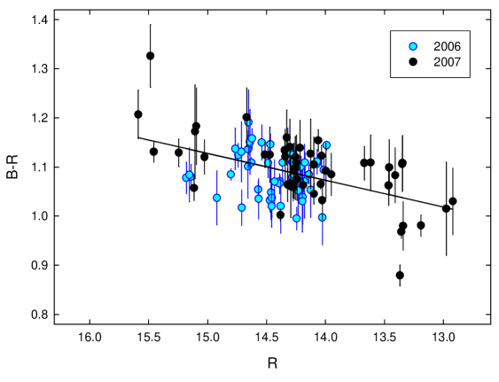
Figure 2: Colour vs. magnitude dependence of 3C 279; data referring to 2006 and 2007 seasons are marked with different colours.

The bluer-when-brighter behaviour is easily seen on Fig. 2 (although it is less evident in the 2006 data). The regression curve is $B-R\propto(0.05\pm 0.01)R$. There are two plausible explanations for the origin of this colour variation: either we observe simultaneously a constant (or slowly varying) source, e.g., the host galaxy and accretion disc, along with a strongly variable source (in the jet) with a substantially different SED; or, alternatively, the bluer-when-brighter trend is intrinsic to the jet, as found for other blazars, especially BL Lac objects (Villata et al. 2000; Raiteri et al. 2003 for 0716+714; Villata et al. 2004a; Papadakis, Villata, & Raiteri 2007 for BL Lacertae). In the following we consider the former supposition as better substantiated for 3C 279 behaviour during these observing seasons.

3.1 Analysis of optical data

Following the technique developed by Hagen-Thorn (see, e.g., Hagen-Thorn et al., 2008, and references therein), let us suppose that the flux changes within some time interval are due to a single variable source. If the variability is caused only by its flux variation but the relative SED remains unchanged, then in the n-dimensional flux space $\{F_{1},...,F_{n}\}$ (n is the number of spectral bands used in multicolour observations) the observational points must lie on straight lines. The slopes of these lines are the flux ratios for different pairs of bands as determined by the SED. With some limitations, the opposite is also true: a linear relation between observed fluxes at two different wavelengths during some period of flux variability implies that the slope (flux ratio) does not change. Such a relation for several bands would indicate that the relative SED of the variable source remains steady and can be derived from the slopes of the lines.

We use magnitude-to-flux calibration constants for optical ($BVRI$) and NIR ($JHK$) bands from Mead et al. (1990), and for UVOT ($V$, $B$, $U$, $W1$, $M2$, $W2$) – from Poole et al. (2008). The Galactic absorption in the direction of 3C 279 was calculated according to Cardelli’s extinction law (Cardelli, Clayton, & Mathis, 1989) and $A_{V}=0\aas@@fstack{m}095$ (Schlegel, Finkbeiner, & Davis, 1998).

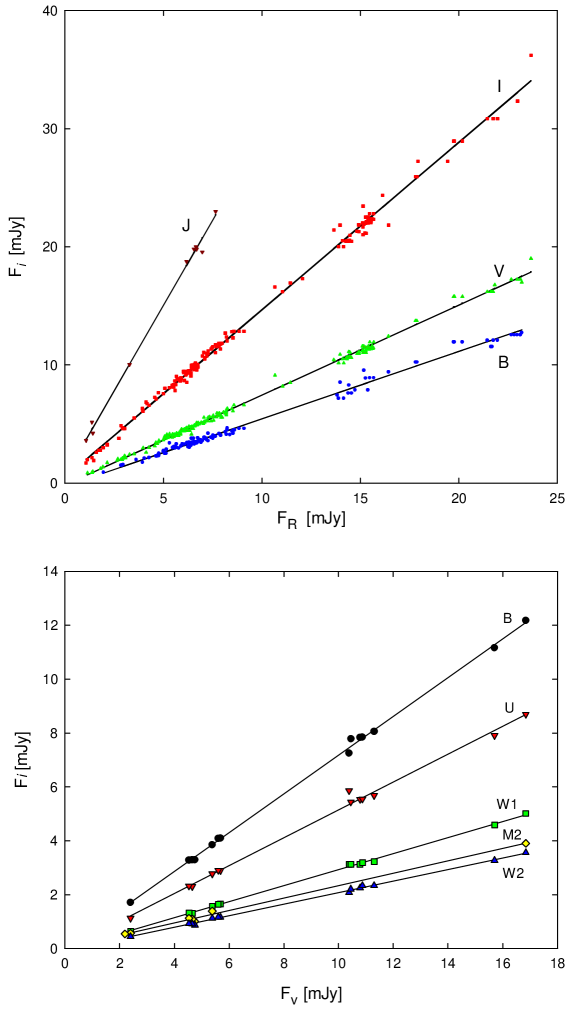
Figure 3: Flux-flux dependences for optical and NIR (top panel) and UVOT bands (bottom panel).

We use the better-sampled $R$-band data to obtain relations in the form of $F_{i}$ vs. $F_{R}$. Similarly, in the case of the UVOT data, we derive $F_{i}$ vs. $F_{V}$.

Figure 3 (upper panel) shows that the method described above holds true: during the entire time covered by our observations, the flux ratios follow linear dependences, $F_{i}=A_{i}+B_{i}\cdot F_{R}$. Values of $B_{i}$, along with the slopes of the regressions, can be used to construct the relative SED of the variable source.

A similar analysis can be carried out with UVOT data. Figure 3 (bottom panel) demonstrates that the same kind of behaviour is seen in the ultraviolet part of the 3C 279 spectrum. This confirms our supposition about self-similar changes in the SED of the variable source.

Table 2: Multicolour properties of the variable optical emission component.

Band	$\log\nu$ (Hz)	$A_{\lambda}$	N	r	$\log B$
(1)	(2)	(3)	(4)	(5)	(6)
Ground-based observations
K	14.1307	0.010	28	0.989	0.8286
H	14.2544	0.016	25	0.998	0.6688
J	14.3733	0.026	10	0.998	0.4609
I	14.5740	0.055	169	0.998	0.1520
R	14.6642	0.076	-	-	0.0000
V	14.7447	0.095	185	0.998	-0.1180
B	14.8336	0.123	121	0.996	-0.2434
UVOT observations
V	14.7445	0.093	-	-	-0.1180
B	14.8407	0.123	14	0.995	-0.2607
U	14.9329	0.147	14	0.999	-0.4045
W1	15.0565	0.195	13	0.999	-0.6438
M2	15.1286	0.285	6	0.949	-0.7306
W2	15.1696	0.271	14	0.998	-0.7856

Columns are as follows: (1) - filter of photometry; (2) - logarithm of the effective frequency of the filter; (3) - extinction at the corresponding wavelength; (4) - number of observations in a given band, (quasi)simultaneous with $R$ (for ground-based observations) and $V$ (for UVOT observations); (5) - correlation coefficient; (6) - logarithm of the contribution of the variable component in the SED at frequency $\nu$ relative to the contribution at $R$ band.

Having found the slopes of flux dependences in the near-IR, optical, and UVOT ranges, we are able to construct the relative SED of the variable source in 3C 279. These results are given in Table 2 (slopes in the UVOT bands are obtained relative to the UVOT $V$ band and fitted to ground-based data) and shown in Fig. 4. (The double $B$-band point is caused by different effective wavelengths for the ground-based telescopes and that of UVOT.) We note that we are unable to judge whether there is only one variable source acting throughout our observations or a number of variable components with the same SED. In any case, in this wavelength range we derive a power-law slope with $\alpha=1.58\pm 0.01$, in the sense $F_{\nu}\propto\nu^{-\alpha}$.

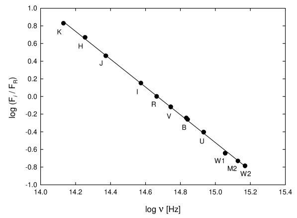
Figure 4: NIR-optical-UV relative spectral energy distribution of 3C 279 variable source(s), normalized to $R$ band.

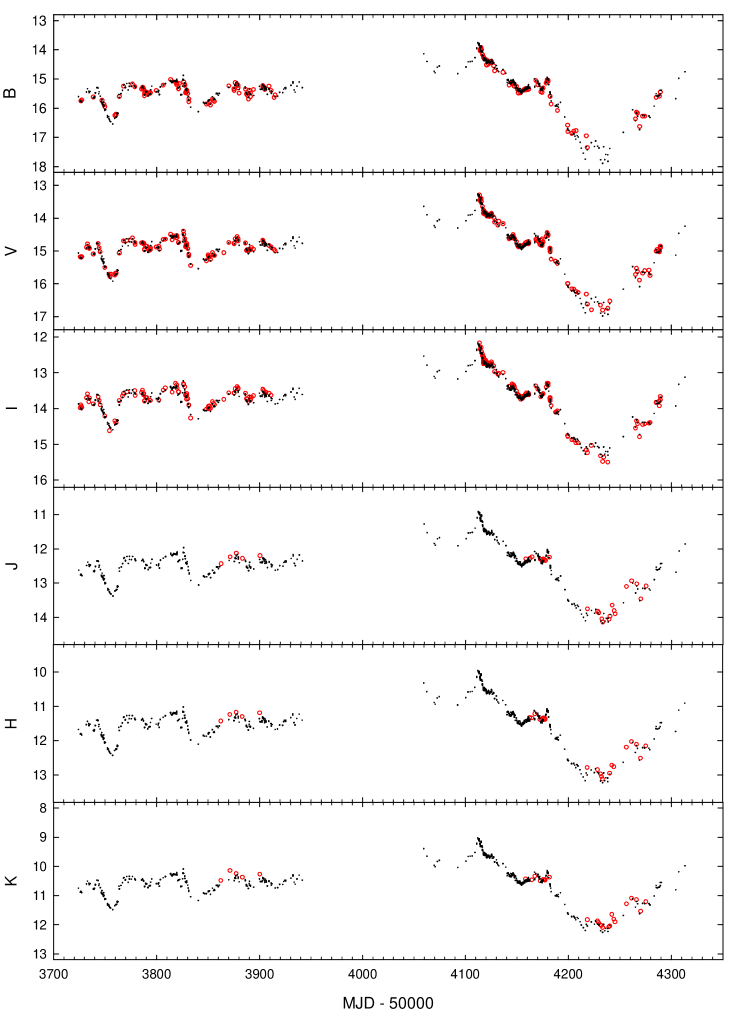
Figure 5: Comparison of observational data (red circles) and calculated values according to dependences shown in Fig. 3 (black dots).

It is possible to “reconstruct” the light curves in the $BVIJHK$ bands using the dependences shown in Fig. 3. This allows us to (1) check the reliability of this procedure and (2) form an impression of the variability behaviour without gaps that otherwise are present in less well-sampled bands. Figure 5 clearly shows that the actual data (red circles) closely match the calculated values (black dots).

Additionally, Figs. 3 and 5 allow us to conclude that there is no noticeable lag between any of the optical and near-infrared light curves; otherwise, we would see both hysteresis loops in Fig. 3 and misfitting in Fig. 5. If any lags in that wavelength range do exist, they are shorter than a few hours. This contradicts the inference drawn by Böttcher et al. (2007) based on a more limited dataset.

3.2 X-ray vs. optical fluctuations

From an analysis of the power spectral density of longer-term monitoring observations, Chatterjee et al. (2008) have concluded that the X-ray light curve of 3C 279 has a red-noise nature, with fluctuations on short time scales having much lower amplitude than those on longer time scales. In general, the X-ray variations are either less pronounced or similar to those at the optical $R$ band. Chatterjee et al. (2008) explain this as the result of the higher energy of electrons that emit optical synchrotron radiation compared to the wide range of energies – mostly lower – of electrons that scatter IR and optical seed photons to the X-ray band. However, we see the opposite occur between MJD 53770 and 53890, when the X-ray fluctuations were more dramatic than those at any of the optical bands (see Fig. 1). (Note: the apparent rapid X-ray fluctuations during the minimum at MJD 54210 to 54240 is mostly noise, since the logarithm of the uncertainty in the fluxes during this time was of order $\pm 0.07$.) We can rule out an instrumental effect as the cause of the rapid X-ray variability, since the X-ray flux of PKS 1510$-$089, measured under very similar circumstances, displays only more modest fluctuations. Although a transient, bright, highly variable X-ray source within $\sim 20^{\prime}$ of 3C 279 could also have caused the observed fluctuations, no such source has been reported previously. Hence, we accept the much more likely scenario that the variations are intrinsic to 3C 279. We discuss a possible physical cause of the rapid X-ray variations in Sect. 8.1.

4 Kinematics and polarization of the radio jet

The Boston University group observes the quasar 3C 279 with the VLBA at 43 GHz monthly (if dynamic scheduling works properly) in a program that started in 2001 (see Chatterjee et al., 2008). Figure 6 shows the sequence of total and polarized intensity images of the parsec-scale jet obtained with the VLBA during 2006-2007. The data were reduced and modelled in the same manner as described in Jorstad et al. (2005). The images are convolved with the same beam, 0.38$\times$0.14 mas at PA=$-9^{\circ}$, corresponding to the average beam for uniform weighting over epochs when all 10 VLBA antennas were in operation (16 epochs out of 22 epochs shown). The images reveal motion of two new components, $C23$ and $C24$ (we follow the scheme of component designation adopted in Chatterjee et al. 2008). Figure 7 plots an angular separation of the components from the core vs. epoch. Although there is some deviation from ballistic motion (especially for $C23$ within 0.3 mas of the core), a linear dependence fits the data according to the criteria adopted by Jorstad et al. (2005). This gives a high apparent speed for both components, $16.5\pm 2.3\leavevmode\nobreak\ c$ and $14.7\pm 0.9\leavevmode\nobreak\ c$, respectively, for $C23$ and $C24$ (for cosmological parameters $H_{\circ}=70$ km s^-1 Mpc^-1, $\Omega_{m}=0.3$, $\Omega_{\lambda}=0.7$), and yields the following times of ejection of components (component’s coincidence with the core): MJD 53888$\pm$55 and 54063$\pm$40. In projection on the plane of the sky, these components move along similar position angles, $PA\sim-114^{\circ}$ and $PA\sim-120^{\circ}$. The directions are different from the position angles of components ejected in 2003-2004, $PA\sim-150^{\circ}$ (Chatterjee et al., 2008), when both the optical and X-ray activity of the quasar was very modest. The images in Fig. 6 contain another moving component about 1 mas from the core ($C21$, Chatterjee et al. 2008), which is a “relic” of the southern jet direction seen near the core during 2004-2005. Using the method suggested in Jorstad et al. (2005), we have estimated the variability Doppler factor, $\delta_{var}$, from the light curves and angular sizes of $C23$ and $C24$, $\delta_{var}=25$ and $\delta_{var}=29$ respectively, with uncertainties $\sim 20\%$. From these values of $\delta_{var}$ and $\beta_{app}$, we derive the Lorentz factor and viewing angle of the jet, $\Gamma=18\pm 5$, $\Theta=2.1^{\circ}\pm 0.3^{\circ}$ for $C23$, and $\Gamma=18\pm 3$, $\Theta=1.6^{\circ}\pm 0.4^{\circ}$ for $C24$. These values are consistent with those derived by Jorstad et al. (2005) during the period 1998–2001 when 3C 279 was in a very active X-ray and optical state, similar to that seen in 2006–07.

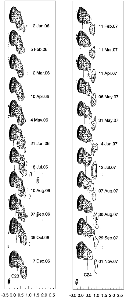
Figure 6: Total intensity VLBA images of 3C 279 at 43 GHz. Line segments within each image indicate the direction of polarization electric vectors, with length proportional to the polarized intensity. The resolution beam is shown by the cross-hatched ellipse in the lower left corner. The contour levels correspond to 0.25,0.5,1,2,4,8,16,32, and 64% of the peak intensity of 17.7 Jy beam^-1. The solid lines indicate the positions of components $C23$ and $C24$ that were ejected in 2006.

Figure 7: Time evolution of angular separations of $C23$ and $C24$ components.

The polarization behaviour in the VLBI core at 7 mm, combined with the jet kinematics discussed above, helps to define the relationship between the physical state of the jet and the multi-waveband variations that we have observed. Figure 8 shows the light curve of the VLBI core at 7 mm and also degree and position angle of polarization in the core. The dotted vertical lines indicate the times of ejection of components $C23$ and $C24$. The ejections of both components in 2006 occurred near maxima in the light curve of the VLBI core region, in keeping with the conclusion of Savolainen et al. (2002) that the emergence of new superluminal knots is responsible for radio flares observed at $\sim 40$ GHz. Each of the ejections in 2006 coincides with the start of a rotation of the EVPA in the core of duration $\sim$60-80 days. During the rotation the degree of polarization in the core reaches a minimum ($<0.5$%). At the end of the rotation, the EVPA in the core aligns with the jet direction (see also Fig. 9).

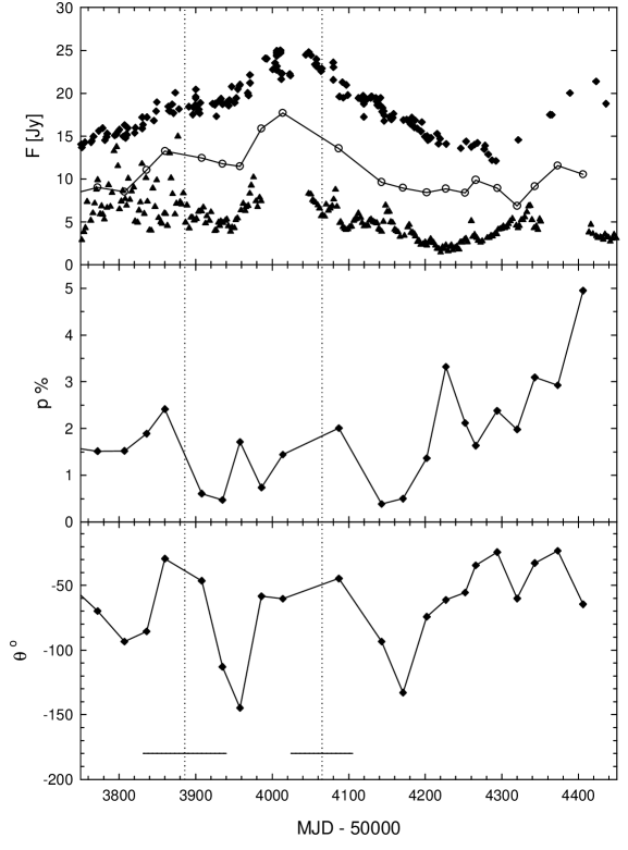
Figure 8: X-ray and radio observations of 3C 279 during 2006-2007. Solid lines mark VLBI core radiation at 7 mm, triangles – X-ray flux (arbitrary units) and diamonds – 37 GHz flux. Vertical dotted lines indicate the times of ejection of components C23 and C24 seen on the VLBA images, and horizontal bars in the bottom panel – uncertainty of the times’ determination.

Figure 8 also presents the X-ray and radio (37 GHz) light curves. The ejections of the components occurred just after maxima in the X-ray light curve. (Although the peak of the second flare is not covered by our observations due to the proximity of the quasar to the Sun, we can infer the approximate time when it occurred by interpolation of the rising and declining phases of the event.) The X-ray maxima lead the ejections by $\sim$60-80 days. The similarity of the behaviour at different wavelengths strongly suggests that the two major flares observed from X-ray to radio wavelengths are associated with disturbances propagating along the jet.

5 Optical Polarimetry

All optical polarimetric data reported here are from the 70cm telescope in Crimea and the 40cm telescope in St.Petersburg, both equipped with nearly identical imaging photometers-polarimeters from St.Petersburg State University. Polarimetric observations were performed using two Savart plates rotated by 45°relative to each another. By swapping the plates, the observer can obtain the relative Stokes $q$ and $u$ parameters from the two split images of each source in the field. Instrumental polarization was found via stars located near the object under the assumption that their radiation is unpolarized. This is indicated also by the high Galactic latitude (57°) and the low level of extinction in the direction of 3C 279 ($A_{V}=0\aas@@fstack{m}095$; Schlegel, Finkbeiner, & Davis 1998).

The results of polarimetric monitoring of 3C 279 during the 2007 campaign are given in Fig. 9, with $R$-band photometry shown in the upper panel for comparison. The most remarkable feature of the polarimetric behaviour is the smooth rotation of the electric-vector position angle (EVPA) of polarization $\theta_{R}$ from the start of the observing season. This rotation continued, while gradually slowing, over approximately two months. In total, the EVPA rotated by $\sim 300\degr$, eventually stabilizing at $\theta_{R}\sim$240°. Note that, because of the $\pm 180$°$n$ ambiguity in $\theta_{R}$, this value is the same as $-120$°, the direction of the VLBA inner jet in 3C 279 during 2007 (cf. Fig. 6). The bottom panel of Fig. 9 also shows the 7mm radio EVPA (red open circles), which rotates along with the optical EVPA, although with fewer points to define the smoothness of the rotation. The degree of optical polarization $p_{R}$ varies more erratically than the EVPA, reaching minimum values of $\sim 2\%$ close to the mid-point of rotation of $\theta_{R}$ and varying between 5% and 30% during the remainder of the observational period.

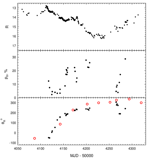
Figure 9: Optical polarimetric data for 3C 279 obtained during the 2007 campaign. EVPA data for the 43 GHz core are marked with red (open) symbols in the bottom panel. The $\pm 180$°$n$ ambiguity in the EVPAs is resolved by requiring the change across contiguous epochs to be $<90$°. No Faraday rotation correction has been applied to the 43 GHz data; see the text.

6 Radio light curves and cross-correlation analysis

The common way to estimate delays between light curves at different wavelengths is to use the DCF (Discrete Correlation Function; Edelson & Krolik 1988; Hufnagel & Bregman 1992). In the case of inter-optical delays, we have mentioned above that there are no lags between any pairs of wavelengths (see Sect. 3.1). This conclusion is confirmed with DCF analysis using different pairs of optical bands – in all the cases the best fit is obtained for 0 days lag. We failed to evaluate DCF lags between optical and radio frequencies for both observational seasons simultaneously, because of the seasonal gap in optical observations caused by solar conjunction and, to a lesser extent, the different time sampling. However, inspection by eye of the optical $R$ and radio light curves (Fig. 10) reveals progressive lags that increase toward lower frequencies, with a time delay between the minima at $R$ band and 37 GHz in mid-2007 of $\sim 60$ days. The dashed slanted lines in Fig. 10 connect the positions of two minima and one maximum that are easily distinguished in the light curves. The question mark in the $R$-band panel denotes the position of a tentative optical maximum, missed due to the seasonal gap. Such behaviour is not unexpected and confirms the results obtained during earlier epochs (e.g., Tornikoski et al., 1994; Lindfors et al., 2006).

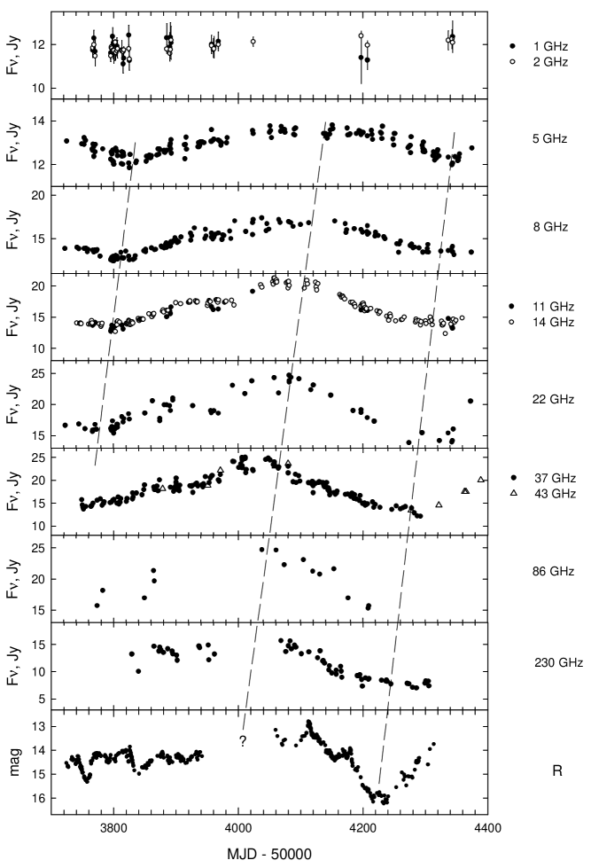
Figure 10: Radio and $R$-band light curves of 3C 279; dashed slanted lines trace mimima and maxima of light curves at different frequencies. Error bars are shown only for 1 and 2 GHz data, where they are larger than symbol size.

We calculated the optical–radio (37 GHz) delays separately for two observing seasons (Fig. 11b). The negative values of delays agree with our conclusion made from eye inspection of Fig. 10. In order to evaluate time lags quantitatively at radio frequencies, we have computed the DCF for the 22 GHz, 14 GHz, 8 GHz and 5 GHz light curves relative to 37 GHz. The results are plotted in Fig. 11c, where vertical bars indicate the lags corresponding to the DCF centroids. Despite the large uncertainties, this plot confirms our conclusion about variations at lower frequencies lagging behind those at high frequencies. Similar results were found by Raiteri et al. (2003) for S5~0716+714, Villata et al. (2004b) for BL~Lac, Raiteri et al. (2005) for AO~0235+164, Villata et al. (2007) for 3C~454.3.

The upper panel of Fig. 11 displays the X-ray–optical DCF. The correlation is rather weak, with changes in the optical ($R$) flux lagging behind X-ray variations by $\sim 1$ day. Inspection by eye suggests that the correlation is strong during 2007 and weak or non-existent in 2006. The most salient feature in the light curves, a deep minimum between MJD 54220 and 54250, occurs essentially simultaneously at both X-ray and optical wavebands. As is discussed by Chatterjee et al. (2008), the X-ray–optical correlation fluctuated slowly over the years from 1996 to 2007, both in strength and in the length and sense of the time lag, with the weakest correlation occurring when the lag is near zero. The latter behaviour matches that observed in 2006–07. The controlling factor may be slight changes in the jet direction over time, which modulates the Doppler factor, light-travel delay across the source, and the position in the jet where the main observed emission originates (Chatterjee et al., 2008).

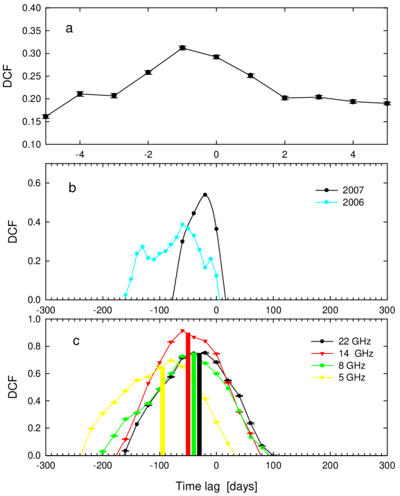
Figure 11: Discrete correlation functions (a) for optical–X-ray, (b) optical–radio (37GHz) and (c) radio frequencies relative to the 37 GHz light curve. Negative time lag corresponds to lower-frequency radiation changing later than at higher frequencies. Vertical bars in panel (c) indicate the lags corresponding to the DCF centroids. Note that in panel (b), due to seasonal gap in optical range, the DCF is calculated separately for the 2006 and 2007 seasons.

7 Spectral energy distribution

Figure 12 displays the spectral energy distribution (SED) of 3C 279 at four different flux levels at epochs when we have sufficient data. Note that the non-variable optical component has not been subtracted in these plots. The overall increase in flux across the entire sampled frequency range strongly suggests that the nonthermal emission at radio through X-ray wavelengths has a common origin, which we identify with the jet based on the appearance of new superluminal knots associated with each of the two major outbursts in flux. The other striking feature of the SEDs is the steepening of the X-ray spectrum at lower flux levels. (Note: the X-ray spectral index is derived from an exponential smoothing of the values obtained from the observations, with a smoothing time of 10 days. This is necessary because of the large uncertainties in individual spectral indices derived when the flux is low.) It is perhaps significant that the highest X-ray spectral index of 1.6 matches that of the variable optical component, while the flattest X-ray spectrum has an index that is lower by 0.5. As we discuss below, this has important implications for the energy gains and losses experienced by the radiating electrons.

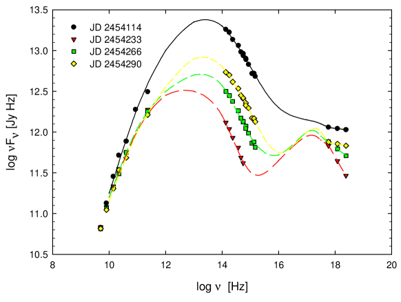
Figure 12: Radio-to-X-ray spectral energy distributions at various epochs in 2007. For each epoch, a cubic spline is drawn through the points. The errors of slope in the X-ray part of SED are of the order of 0.1.

8 Discussion

8.1 Variability in flux and continuum spectrum

During the two observing seasons reported here, 3C 279 exhibited flux variations from radio to X-ray wavelengths (see Fig. 1). We observed the shortest time scales of variability, $\Delta t/\ln(F_{\rm max}/F_{\rm min})\sim$ days, in the X-ray and optical bands. There were two deep minima in the X-ray light curve, the first (at the start of 2006) coinciding with a low optical state with at least two closely spaced minima, and the second essentially simultaneous with a deep optical minimum between MJD 54210 and 54240. The discrete cross-correlation function indicates that the time lag between the X-ray and optical bands is essentially zero.

The SEDs in Fig. 12 demonstrate that the X-ray emission is not simply a continuation of the optical synchrotron spectrum. This agrees with the conclusion of Chatterjee et al. (2008) that the X-rays result from synchrotron self-Compton (SSC) scattering. During the highest flux state, the X-ray spectral index was $\alpha_{x}=1.1$, while the optical spectral index of the variable component was $\alpha_{\rm opt}=1.6$ throughout both observing seasons (see Fig. 4). This can be accommodated within a standard nonthermal source model if there is continuous injection of relativistic electrons with a power-law energy distribution of slope $-3.2$ that is steepened to $-4.2$ at high energies by radiative energy losses. This implies that there is a flatter spectrum at mid- and far-IR wavelengths, below $\sim 10^{14}$ Hz, with $\alpha_{\rm IR}=1.1$ that matches that of the high flux state. At minimum flux, the X-ray spectrum steepens to $\alpha_{x}=1.6=\alpha_{\rm opt}$.

The steep X-ray spectrum during the flux minimum of 2007 implies that the entire synchrotron spectrum above the spectral turnover frequency had a steep spectral index of 1.6. In the context of the standard nonthermal source model mentioned above, essentially all of the electrons suffered significant radiative energy losses at the time of the low state. That is, their radiative loss time scale was shorter than the time required for them to escape from the emission region. For this to be the case, the injected energy distribution must have a low-energy cutoff that is far above the rest-mass energy. We can match the time scale of optical and X-ray variability of 3C 279 if we adopt a magnetic field strength in the emission region of $B\sim 1$ G. Electrons radiating at the UV wavelengths must then have a Lorentz factor $\gamma\equiv(E/mc2)\sim 6000B^{-1/2}(\delta/25)^{-1/2}$, those radiating at a break frequency of $\sim 10^{14}$ Hz have $\gamma\sim 1500B^{-1/2}(\delta/25)^{-1/2}$, and those emitting at $10^{12}$ Hz have $\gamma\sim 150B^{-1/2}(\delta/25)^{-1/2}$. Given the turnover in the SED at $\sim 10^{12}$ Hz (cf. Fig. 12), we assume that either the variable emitting component becomes self-absorbed near this frequency or that there is a lower-energy cutoff (or sharp break) in the injected electron energy distribution at $\gamma\sim 150B^{-1/2}(\delta/25)^{-1/2}$. The time scale for energy losses from synchrotron radiation, as measured in our reference frame, is $\sim 4B^{-3/2}(\delta/25)^{-1/2}$ days at $\sim 10^{12}$Hz if we adopt a Doppler factor of 25 (see Sect. 4 above). This is similar to the minimum X-ray variability time scale that we observed. The time scale for synchrotron energy losses allows the variability at optical bands to be as fast as $\sim 3$ hours as long as the emission region is smaller than $\sim 5\times 10^{15}(\delta/25)$ cm.

The 2.4–10 keV X-ray emission results from a range of seed photons scattered by electrons having a range of energies (McHardy et al., 1999). If there is a break in the spectrum, as we infer, then the bulk of the X-ray emission is from seed photons at frequencies below the break – $\nu\sim 10^{12}$–$10^{14}$ Hz – scattered by electrons with energies below the break – $\gamma\sim$ 150–1500. The rapid optical variability in the low flux state implies that the magnetic field remained of similar strength as for the high state. However, the break frequency must have decreased to nearly $10^{12}$Hz for the SSC X-ray spectrum to have steepened to $\alpha_{x}=\alpha_{\rm opt}=1.6$. This could occur simply from adiabatic cooling if the emission region expanded by a factor of 10 between the high and low states. However, in this case the magnetic field would have dropped, increasing the time scale of variability and decreasing the flux by more than the observed factor of $\sim 10$ (cf., e.g., Marscher & Gear, 1985). Alternatively, the time for electrons to escape the emission region could have increased as the flux declined. For example, in the shock model of Marscher & Gear (1985), the electrons are accelerated at the shock front and advect toward the rear of the shocked region until they encounter a rarefaction at a distance $x$ behind the shock. If the primary energy loss is due to synchrotron radiation, the break frequency $\nu_{b}\propto x^{-2}B^{-3}$. A factor of 10 increase in the extent (in the direction parallel to the jet axis) of the shocked region would then cause the break frequency to decrease from $\sim 10^{14}$ to $10^{12}$ Hz. However, this would require a high relative velocity between the shock front and the rear of the shocked region, implying that the emission near the latter is relatively poorly beamed and therefore not prominent.

Another possibility, which seems less contrived, is that the X-ray emission during the flux minimum is not the decayed remnant of the previous event, but rather comes from the new component that caused the outburst seen during the last $\sim 100$ days of the 2007 observing season. This component would first be seen well upstream of the location where the flux reaches a maximum, and therefore the external photon field from the broad emission-line region and dusty torus would initially be higher than at later times (see Sokolov & Marscher, 2005). In this case, the break frequency would increase with time as the component moves downstream and the level of inverse Compton energy losses decreases. This scenario predicts that there should be a $\gamma$-ray flare from inverse Compton scattering of seed photons originating outside the jet prior to the main outburst. Although the $\gamma$-ray observations needed to test this were not undertaken in early May 2007 (the newly-launched AGILE telescope was in the testing phase), future observations involving GLAST and AGILE will determine whether such precursor flares actually occur.

The higher amplitude of variability at X-ray energies relative to the optical bands between MJD 53770 and 53890 could be the result of the higher sensitivity of the SSC vs. the synchrotron flux to changes in the number of relativistic electrons (quadratic vs. linear dependence). Although, as discussed above, the X-rays during high flux states are scattered seed photons that originally had a range of frequencies from $\sim 10^{12}$ to $10^{14}$ Hz, the longest time scale of variability – a few days at $10^{12}$ Hz – is short enough to be consistent with the observations. Alternatively, variable optical depths within the emitting region could cause the density of SSC seed photons at frequencies $\sim 10^{12}$ Hz to fluctuate without changing the observed synchrotron radiation much, thereby causing the SSC X-rays to be more highly variable than the optical synchrotron radiation.

The continuum spectrum from UV to near-IR wavelengths is well described by a power law with constant spectral index $\alpha_{\rm opt}=1.6$, even as the flux varied by over an order of magnitude. As discussed above, this agrees with constant injection of relativistic electrons with a power-law energy distribution of slope $-3.2$ that is steepened to $-4.2$ at high energies by radiative energy losses. Although such steep slopes are not in conflict with particle acceleration models, neither are they predicted. Yet the constancy of this steep slope during the campaign implies that the physical parameters governing the particle acceleration process can be maintained over long periods of time and from one event in the jet to the next. This presents a challenge to theories for particle acceleration.

The radio light curves from 230 to 1 GHz become progressively smoother with decreasing frequency. As can be inferred from Fig. 10, there is also a lag in the timing of maxima and minima in the light curves toward lower frequencies, as well as a delay of 100–150 days between optical variations and those at 5 GHz. This is readily explained as a consequence of opacity, with an outburst delayed at radio frequencies until the disturbance reaches the location in the jet where the optical depth is less than unity (see, e.g., Hughes, Aller, & Aller, 1985; Marscher & Gear, 1985). In addition, the radiative lifetime of electrons in the radio-emitting regions is longer than is the case farther upstream, owing to the lower magnetic field and photon energy density. This prolongs the duration of an outburst – and therefore the timing of the minima in the light curves – at lower frequencies. Because of the absence of optical and 230 GHz data near the global peak in 2006-07, we cannot determine whether there is a significant delay between the optical and 230 GHz light curves. However, the fact that at the end of the campaign period we see a brightening in the optical, but not in the mm light curve, suggests that the two emission regions are not co-spatial.

8.2 Polarimetric behaviour

The main feature of interest in the polarimetric data is the rotation of the $R$-band and 43 GHz core EVPAs between MJD 54120 and 54200 (see Fig. 9). The optical polarization was several percent or less during the middle of this rotation, but it was as high as 23% near the beginning and end. Apparent rotations by $\sim 300$°or more can occur simply from random walks caused by turbulent cells with random magnetic field orientation passing through the emission region (Jones, 1988). In this case, however, the apparent rotation has an extremely low probability to be as smooth as we have observed (D’Arcangelo et al., 2007). We therefore conclude that the rotation is intrinsic to the jet. The coincident rotation of the 43 GHz core and optical polarization vector suggests a common emission site at the two wavebands. [Note: the discrepancy between 43 GHz and optical EVPAs measured at essentially the same time could be due to Faraday rotation, which is of the order of tens of degrees and might vary with location (Zavala & Taylor, 2004; Jorstad et al., 2007).]

The observed behaviour is qualitatively similar to the models suggested by Kikuchi et al. (1988); Sillanpää et al. (1993); Marscher et al. (2008), where a shock wave or other compressive feature propagating down the jet traces a spiral path and cycles through the orientations of an underlying helical magnetic field. This manifests itself through rotation of the position angle of linear polarization as the feature moves outward. The polarization is low during the rotation because the symmetry of the toroidal component of the helical magnetic field produces a cancellation of the net linear polarization when integrated over the entire structure of the feature. On the other hand, the cancellation is only partial, which implies that the feature does not extend over the entire cross-section of the jet.

Several documented events of optical position angle rotation have been reported by Sillanpää et al. (1993) and Marscher et al. (2008) (both – BL~Lac), Kikuchi et al. (1988) (OJ287), and Larionov et al. (2008) (S5~0716+71). The time scale of rotation of the polarization vector in 3C 279 is much longer than in any of these previous cases – almost two months as compared to $\sim 1$ week. This difference can be explained by the substantially larger scale of the core of the 3C 279 jet as well as the greater distance from the central engine (as determined by the intrinsic opening angle of the jet of $0.4$°$\pm 0.2$°; Jorstad et al., 2005). The time required for the disturbance to reach and pass through the millimeter-wave core is therefore longer than in the other blazars.

The first superluminal knot that emerged during our campaign (see Fig. 8) was located at the centroid of the 43 GHz core on MJD 53888$\pm$55. (It is interesting that this coincided with the end of the interval of rapid fluctuations of the optical and, especially, X-ray flux.) The flux subsequently rose at all wavebands, reaching a peak $\sim 130$ days later. We note that the EVPA of the core at 43 GHz changed by $\sim 130$° as the flux rose, although the data are too sparse to determine whether this was a smooth rotation. The next knot coincided with the core on MJD 54063$\pm$40, $\sim 50$ days after the radio and X-ray flux peak but at a time of multiple, major optical flares. This was shortly before the start of the optical EVPA rotation featured in Fig. 9. The timing suggests that the optical flares and EVPA rotation in early 2007 took place in this knot as it moved downstream of the core. This contrasts with the case of BL Lac, in which the region with helical magnetic field lies upstream of the millimeter-wave core. This led Marscher et al. (2008) to associate the helical field with the acceleration and collimation zone (ACZ) of the jet flow, downstream of which the flow is turbulent. For the polarization rotation to occur downstream of the 43 GHz core, either the core lies within the ACZ in 3C 279 or the helical field can persist beyond the ACZ. The latter possibility is favoured by Gabuzda et al. (2008) based on circular polarization observations of blazars. The downward curvature of the EVPA vs. time curve of Fig. 9 implies that the pitch angle of the helix becomes smaller – i.e., the helix opens up – with distance from the core. The time scale for this to occur $\sim 60$ days, which corresponds to a distance of $\sim 20$ pc along the jet of 3C 279, given the kinematics and angle to the line of sight of the jet derived in Sect. 4.

9 Conclusions

By following the evolution of the flux at radio, near-IR, optical, UV, and X-ray frequencies and the linear polarization at radio and optical bands intensely over a two-year period, we have uncovered patterns that reveal key aspects of the physics in the relativistic jet in 3C 279. The IR-optical-UV continuum spectrum of the variable component follows a power law with a constant slope of $-1.6$, while that in the 2.4–10 keV X-ray band varies in slope from $-1.1$ to $-1.6$. This agrees with the expectations of an emission region into which electrons are steadily injected with a power-law energy distribution of slope $-3.2$ that is modified to a slope of $-4.2$ at high energies owing to radiative losses. The steepest X-ray spectrum occurs at a flux minimum. The least contrived explanation is that the X-ray emission at this time comes from a new component in an upstream section of the jet where the radiative losses from inverse Compton scattering of seed photons from the broad emission-line region are important. If this is the case, then a $\gamma$-ray flare should precede the rising portion of a multi-waveband outburst, a prediction that can be tested with GLAST and AGILE along with intensive multi-waveband monitoring.

During the decline of flux from the maximum in early 2007, we observe a rotation of the optical and 43 GHz core polarization vectors totaling $\sim 300$°. The smoothness of the rotation leads us to conclude that, as in BL Lac (Marscher et al., 2008) and possibly other blazars, the jet contains a helical magnetic field. However, in contrast with BL Lac, the region of helical field in 3C 279 extends $\sim 20$ pc past the 43 GHz core. Given the paucity of well-sampled optical polarization monitoring over periods of time longer than 1–2 weeks, such rotations may be the norm in blazars. If so, more extensive future polarization monitoring should uncover many more examples, allowing more general inferences to be drawn regarding the magnetic field structure in jets and its relationship to the dynamics of the flow.