IPhT-T08/164

A holomorphic and background independent partition function

for matrix models and topological strings

Bertrand Eynard^a and Marcos Mariño^b

 ^a Institut de Physique Théorique, CEA, IPhT

F-91191 Gif-sur-Yvette, France

CNRS, URA 2306, F-91191 Gif-sur-Yvette, France

eynard@spht.saclay.cea.fr

 ^bSection de Mathématiques et Département de Physique Théorique

Université de Genève, CH-1211 Genève, Switzerland

marcos.marino@unige.ch

Abstract

We study various properties of a nonperturbative partition function which can be associated to any spectral curve. When the spectral curve arises from a matrix model, this nonperturbative partition function is given by a sum of matrix integrals over all possible filling fractions, and includes all the multi-instanton corrections to the perturbative $1/N$ expansion. We show that the nonperturbative partition function, which is manifestly holomorphic, is also modular and background independent: it transforms as the partition function of a twisted fermion on the spectral curve. Therefore, modularity is restored by nonperturbative corrections. We also show that this nonperturbative partition function obeys the Hirota equation and provides a natural nonperturbative completion for topological string theory on local Calabi–Yau threefolds.

1 Introduction

The perturbative partition function of a matrix model with fixed filling fractions $\epsilon$ has the form

$$Z=\exp\Bigl{\{}\sum_{g=0}^{\infty}N^{2-2g}F_{g}(\epsilon)\Bigr{\}},$$ (1.1)

where $F_{g}(\epsilon)$ is the generating function for fatgraphs of genus $g$ [19]. The same structure appears in the partition function of closed topological string theory, where $1/N$ becomes the string coupling constant $g_{s}$ and the $\epsilon$ become closed string moduli. In both cases, the partition function depends on a choice of background $\epsilon$.

The background dependence of $Z$ is closely related to its behavior under the modular group of the theory. In the context of matrix models, the large $N$ limit is described by an algebraic curve called the spectral curve, and the modular group is simply the symplectic group ${\rm Sp}(2\bar{g},{\mathbb{Z}})$, where $\bar{g}$ is the genus of the spectral curve (not to be confused with the genera $g$ appearing in the topological expansion). In topological string theory on a Calabi–Yau threefold $X$, the modular group is the symplectic group ${\rm Sp}(2n,{\mathbb{Z}})$ of symmetries which preserve the symplectic form, where $n=b_{3}(X)/2$. The mathematical manifestation of background dependence is that, as emphasized in [1], the partition function $Z$ does not have good transformation properties under the modular group of the theory. In fact, as shown in [1] in topological string theory and in [25] in the context of matrix models, the $F_{g}$ transform as quasi-modular forms, with shifts (the prototype for this behavior is the second Eisenstein series).

It is possible to restore modularity of $F_{g}$ (hence of $Z$) at the price of introducing a non-holomorphic dependence on $\bar{\epsilon}$. When this is done, the resulting partition function $Z(\epsilon,\bar{\epsilon})$ satisfies the holomorphic anomaly equations of [8]. In the context of matrix models this was shown in [24]. Indeed, the holomorphic anomaly was interpreted in [48] as an obstruction to background independence. Therefore, the lack of background independence seems to face us with a choice between modularity and holomorphicity.

In the case of matrix models, it is however clear that the original matrix integral which leads to the above $1/N$ expansion can not depend on the choice of filling fractions. It should only depend on the coupling constants of the potential, the rank of the matrix $N$, and a choice of integration path for the eigenvalues. Therefore, for matrix models, background dependence is an artifact of the $1/N$ expansion, coming from the fact that one has chosen a particular saddle configuration at large $N$. Background independence should be restored by including the rest of the saddle points in an appropriate way, i.e. by including the instanton configurations of the matrix model. In this sense, matrix integrals provide a simple framework in which we might understand both the breakdown of background independence and the appropriate mechanism to restore it.

In [22], one of us proposed an asymptotic formula for the partition function of convergent matrix integrals, generalizing the results of [11]. This formula includes, together with the perturbative expansion (1.1), a series of nonperturbative corrections which can be interpreted in terms of instantons of the matrix model. Since this nonperturbative partition function is obtained by summing over all possible filling fractions, it was suggested in [22] that it gives a natural proposal for a background independent partition function.

As in the case of the $F_{g}$ [25], the nonperturbative partition function introduced in [22] can be defined for any spectral curve $\Sigma$. On top of the spectral curve data, one also needs a choice of characteristics $(\mu,\nu)$, just as for theta functions on a Rieman surface. These characteristics encode nonperturbative information; for example, in a matrix model they encode the choice of integration contour for the eigenvalues. In this paper we study in detail the transformation properties of the nonperturbative partition function $Z_{\Sigma}(\mu,\nu;\epsilon)$ under the modular group. It turns out that they have good modular properties. More precisely, they transform in a matrix representation of the modular group, i.e.

$$\tilde{Z}_{\Sigma}(\tilde{\mu},\tilde{\nu};\tilde{\epsilon})=\zeta\bigl{[}^{\mu}_{\nu}\bigr{]}(\Gamma)Z_{\Sigma}(\mu,\nu;\epsilon),$$ (1.2)

where $\zeta\bigl{[}^{\mu}_{\nu}\bigr{]}(\Gamma)$ is a phase depending on the characteristics $\mu$, $\nu$ and the modular transformation $\Gamma$, and $\tilde{\mu},\tilde{\nu}$ are new, transformed characteristics. Both $\zeta\bigl{[}^{\mu}_{\nu}\bigr{]}(\Gamma)$ and $\tilde{\mu},\tilde{\nu}$ are the same quantities which appear in the transformation properties of higher rank theta functions. Since $Z_{\Sigma}(\mu,\nu;\epsilon)$ is manifestly holomorphic, we obtain a partition function which is holomorphic, modular, and background independent. In other words, modularity can be restored in a holomorphic way by including nonperturbative effects. Notice that, according to (1.2), $Z_{\Sigma}(\mu,\nu;\epsilon)$ transforms like a twisted fermion on the Riemann surface, with twists given by the characteristics $\mu,\nu$. Therefore, it seems to be the most natural object from the point of view of the free fermion theory on $\Sigma$ advocated in [2, 18] and many other papers. As in CFT, one can also regard the $Z_{\Sigma}(\mu,\nu;\epsilon)$ as chiral conformal blocks which can be used to construct invariants under suitable subgroups of the modular group.

We also show that the nonperturbative partition function is a tau function, in the sense that it satisfies a Hirota-type equation. This was observed in [25] in the case of genus zero spectral curve, where the nonperturbative instanton corrections are absent. Here we show that the inclusion of these corrections makes possible to generalize the construction of [25] to any spectral curve.

Since the construction of $Z_{\Sigma}(\mu,\nu;\epsilon)$ only needs data coming from $\Sigma$, the nonperturbative partition function introduced in [22] can be also defined for topological strings on a variety of local Calabi–Yau manifolds, including mirrors of toric Calabi–Yau’s. In fact, it has been advocated in [41, 40] that the nonperturbative topological string partition function should include matrix model-like instanton effects, and in [40] it was pointed out that the nonperturbative partition function of [22] appears naturally in topological string models with large $N$ Chern–Simons theory duals. Therefore, these nonperturbative partition functions provide homolorphic, modular and background independent partition functions for a wide class of topological string theory models.

The organization of this paper is as follows. In section 2 we recall the definition of the nonperturbative partition function introduced in [22], and we stress the fact that it can be associated to any spectral curve. In section 3, which is the core of the paper, we show in detail that this partition function has good transformation properties under the modular group. In section 4 we review how the nonperturbative partition function appears in the context of matrix models, by summing over filling fractions. In section 5 we discuss the applications to topological string theory on local Calabi–Yau manifolds, and we propose that the nonperturbative partition function gives a natural nonperturbative object for topological strings. In section 6 we analyze the integrability properties and we show that $Z_{\Sigma}(\mu,\nu;\epsilon)$ is a tau function. Finally, in section 7 we list some conclusions and avenues for further research.

2 The nonperturbative partition function

Consider an arbitrary “spectral curve” $\Sigma=({\cal C},x,y)$, i.e. the data of a compact Riemann surface ${\cal C}$ of genus $\bar{g}$, together with two analytical functions $x,y$ on some open domain of ${\cal C}$. Its symplectic invariants $F_{g}$’s were defined in [25] (and we recall the definition in appendix A). They are such that (if $g\geq 2$):

$$F_{g}({\cal C},x,\lambda y)=\lambda^{2-2g}\,F_{g}({\cal C},x,y),$$ (2.1)

and if two spectral curves have the same symplectic form ${\rm d}{\tilde{x}}\wedge{\rm d}{\tilde{y}}={\rm d}x\wedge{\rm d}y$, we have

$$F_{g}({\cal C},{\tilde{x}},{\tilde{y}})=F_{g}({\cal C},x,y).$$ (2.2)

For the spectral curve $\Sigma=({\cal C},x,y)$, the nonperturbative partition function introduced in [22] in the context of matrix models, by summing over filling fractions (see section 4 for more details on the origin of this definition), is defined by

$$Z_{\Sigma}(\mu,\nu;\epsilon)={{\rm e}^{\sum_{g\geq 0}N^{2-2g}F_{g}(\epsilon)}}\sum_{k}\sum_{l_{i}>0}\sum_{h_{i}>1-{l_{i}\over 2}}{N^{\sum_{i}(2-2h_{i}-l_{i})}\over k!l_{1}!\,\dots\,l_{k}!}\,\,\,F_{h_{1}}^{(l_{1})}\dots F_{h_{k}}^{(l_{k})}\,\,\Theta_{\mu,\nu}^{(\sum_{i}l_{i})}(NF^{\prime}_{0},\tau)$$ (2.3)

$$\quad={{\rm e}^{N^{2}F_{0}}}\,{{\rm e}^{F_{1}}}\,{{\rm e}^{(N^{-2}F_{2}+N^{-4}F_{3}+\dots)}}\,\,\biggl{\{}\Theta_{\mu,\nu}+{1\over N}\Bigl{(}\Theta^{\prime}_{\mu,\nu}F_{1}^{\prime}+{1\over 6}\Theta_{\mu,\nu}^{\prime\prime\prime}\,F_{0}^{\prime\prime\prime}\Bigr{)}$$

$$\quad+{1\over N^{2}}\Bigl{(}{1\over 2}\Theta_{\mu,\nu}^{\prime\prime}F_{1}^{\prime\prime}+{1\over 2}\Theta_{\mu,\nu}^{\prime\prime}F_{1}^{\prime 2}+{1\over 24}\Theta_{\mu,\nu}^{(4)}F_{0}^{\prime\prime\prime\prime}+{1\over 6}\Theta_{\mu,\nu}^{(4)}F_{0}^{\prime\prime\prime}F_{1}^{\prime}+{1\over 72}\Theta_{\nu,\mu}^{(6)}F_{0}^{\prime\prime\prime 2}\Bigr{)}+\dots\biggr{\}}.$$

In this partition function, the $F_{g}$’s are the symplectic invariants [25] of the spectral curve $\Sigma$, their derivatives are with respect to the background filling fraction $\epsilon$ and computed at:

$$\epsilon={1\over 2\pi{\rm i}}\,\oint_{{\cal A}}y{\rm d}x,$$ (2.4)

and the $F_{g}({\cal C},x,y)$’s and their derivatives depend on a choice of symplectic basis of $2\bar{g}$ one-cycles ${\cal A}_{i},{\cal B}_{j}$ on ${\cal C}$. Finally, the theta function $\Theta_{\mu,\nu}$ of characteristics $(\mu,\nu)$ is defined by

$$\Theta_{\mu,\nu}(u,\tau)=\sum_{n\in{\mathbb{Z}}^{\bar{g}}}{{\rm e}^{(n+\mu-N\epsilon)u}}\,\,{{\rm e}^{\pi{\rm i}(n+\mu-N\epsilon)\tau(n+\mu-N\epsilon)}}\,\,{{\rm e}^{2{\rm i}\pi n\nu}}$$ (2.5)

and is evaluated at

$$u=NF_{0}^{\prime},\qquad F^{\prime}_{0}=\oint_{{\cal B}}y(x){\rm d}x,\qquad\tau={1\over 2\pi{\rm i}}F_{0}^{\prime\prime}.$$ (2.6)

In (2.3), the derivatives of the theta function (2.5) are w.r.t. $u$, therefore each derivative introduces a factor of $n+\mu-N\epsilon$ in the sum (2.5). The derivatives of $\Theta$ and the derivatives of $F_{g}$, are written with tensorial notations. For instance, ${1\over 6}\Theta_{\mu,\nu}^{(4)}F_{0}^{\prime\prime\prime}F_{1}^{\prime}$ actually means:

$${1\over 6}\Theta_{\mu,\nu}^{(4)}F_{0}^{\prime\prime\prime}F_{1}^{\prime}\equiv{1\over 2!\,3!\,1!}\,\,\sum_{i_{1},i_{2},i_{3},i_{4}}\,{\partial^{4}\Theta_{\mu,\nu}\over\partial u_{i_{1}}\partial u_{i_{2}}\partial u_{i_{3}}\partial u_{i_{4}}}\,\,{\partial^{3}F_{0}\over\partial\epsilon_{i_{1}}\partial\epsilon_{i_{2}}\partial\epsilon_{i_{3}}}\,\,{\partial F_{1}\over\partial\epsilon_{i_{4}}}$$ (2.7)

and the symmetry factor (here ${1\over 6}={2\over 2!\,3!\,1!}$) is the number of relabellings of the indices, giving the same pairings, and divided by the order of the group of relabellings, i.e. $k!\,l_{1}!\dots l_{k}!$, as usual in Feynmann graphs.

The $\Theta$ function is closely related to the standard theta function, which is defined by

$$\vartheta\bigl{[}^{\mu}_{\nu}\bigr{]}(\xi|\tau)=\sum_{{\bf n}\in{\mathbb{Z}}^{\bar{g}}}\exp\bigl{[}{\rm i}\pi(n+\mu)\tau(n+\mu)+2\pi{\rm i}(n+\mu)(\xi+\nu)\bigr{]}.$$ (2.8)

It it easy to see that these two functions are related as follows

$$\Theta_{\mu,\nu}(u,\tau)=\exp\biggl{[}-N^{2}\Bigl{(}\epsilon F_{0}^{\prime}+{1\over 2}\epsilon^{2}F_{0}^{\prime\prime}\Bigr{)}\biggr{]}\,\,\vartheta\bigl{[}^{\mu}_{\nu}\bigr{]}(\xi|\tau)$$ (2.9)

where

$$\xi={N\over 2\pi{\rm i}}\oint_{{\cal B}-\tau{\cal A}}y(x){\rm d}x=N\biggl{(}{F^{\prime}_{0}\over 2\pi{\rm i}}-\tau\epsilon\biggr{)}.$$ (2.10)

Finally, we point out that, as shown in [22], the $1/N$ corrections in (2.3) can be resummed in terms of a single theta function, and $Z_{\Sigma}(\mu,\nu;\epsilon)$ can be written as

$$Z_{\Sigma}(\mu,\nu;\epsilon)={{\rm e}^{\sum_{g\geq 0}N^{2-2g}F_{g}(\epsilon)}}\Theta_{\mu,\nu}(u^{N},\tau^{N}),$$ (2.11)

where

$$u^{N}=NF_{0}^{\prime}\bigl{(}1+{\cal O}(1/N^{2})\Bigr{)},\quad\tau^{N}=\tau+{\cal O}(1/N^{2}),$$ (2.12)

and the corrections (which depend on the $F_{g}$) can be easily determined order by order in $1/N$.

3 Modular properties of the nonperturbative partition function

In this section we discuss the transformation properties of the nonperturbative partition function (2.3) under the modular group. For that purpose, we shall first remind the transformation properties of the $F_{g}$’s and their derivatives, and then the transformation properties of the $\Theta$-function. For simplicity, we will first discuss the case in which $\bar{g}=1$ and the theta functions involved are of rank one. There are little changes when we go to the general case, but we will indicate these in section 3.3 below.

For spectral curves of $\bar{g}=1$, a general modular transformation is an element of ${\rm SL}(2,{\mathbb{Z}})$,

$$\Gamma=\begin{pmatrix}\alpha&\beta\\ \gamma&\delta\end{pmatrix}\in{\rm SL}(2,{\mathbb{Z}}),$$ (3.1)

where $\alpha,\beta,\gamma,\delta\in{\mathbb{Z}}$ and $\alpha\delta-\gamma\beta=1$. Under this transformation the integrals of $y{\rm d}x$ over the ${\cal B}$ and the ${\cal A}$ cycles transform as

$$\begin{pmatrix}F^{\prime}_{0}\\ 2\pi{\rm i}\epsilon\end{pmatrix}\rightarrow\begin{pmatrix}{\tilde{F}}^{\prime}_{0}\\ 2\pi{\rm i}{\tilde{\epsilon}}\end{pmatrix}=\begin{pmatrix}\alpha&\beta\\ \gamma&\delta\end{pmatrix}\,\begin{pmatrix}F^{\prime}_{0}\\ 2\pi{\rm i}\epsilon\end{pmatrix}.$$ (3.2)

It follows that

$${\tilde{\tau}}={\alpha\tau+\beta\over\gamma\tau+\delta},\qquad\tilde{\xi}={\xi\over\gamma\tau+\delta},$$ (3.3)

so in particular $\xi$ is a modular form of weight $-1$.

3.1 Modular transformations of the perturbative amplitudes

The transformation properties of the genus zero free energy $F_{0}$ can be derived from those of $F_{0}^{\prime}$ by integration, and they read

$$\tilde{F}_{0}=F_{0}+{1\over 2}\delta\beta(2\pi{\rm i}\epsilon)^{2}+{1\over 2}\gamma\alpha(F_{0}^{\prime})^{2}+\beta\gamma(2\pi{\rm i}\epsilon)F_{0}^{\prime}.$$ (3.4)

This implies that the combination

$${\tilde{F}}_{0}-{1\over 2}{\tilde{\epsilon}}\,{\tilde{F}}^{\prime}_{0}=F_{0}-{1\over 2}\epsilon\,F^{\prime}_{0}$$ (3.5)

stays invariant.

Another transformation property which will be useful in the following is that

$$2\pi{\rm i}\epsilon(F_{0}^{\prime}-2\pi{\rm i}\epsilon\tau)\rightarrow 2\pi{\rm i}\epsilon(F_{0}^{\prime}-2\pi{\rm i}\epsilon\tau)-\kappa(F_{0}^{\prime}-2\pi{\rm i}\tau\epsilon)^{2},$$ (3.6)

where

$$\kappa=-(\gamma\tau+\delta)^{-1}\,\gamma.$$ (3.7)

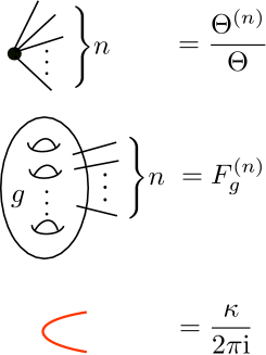
Figure 1: We will represent the different ingredients appearing in the modular transformation of the nonperturbative partition function by the graphic symbols depicted above.

The transformation properties for the $F_{g}$, $g\geq 1$ were studied in [1] from the point of view of topological string theory. [1] also found an elegant diagrammatic formalism to express these transformations. The formalism can be depicted as follows: after a modular transformation, $F_{g}$ gets contributions corresponding to all possible stable degenerations of a genus $g$ Riemann surface. Degenerations are obtained by pinching a non-trivial cycle. A stable degenerate surface is a nodal surface with marked points whose components have strictly negative Euler characteristics. Each degenerate cycle becomes a nodal point, and carries a factor $(2{\rm i}\pi)^{-1}\kappa$. For example, the modular transformation of $F_{2}$ gets contributions corresponding to pinching either 1,2 or 3 cycles. This leads to the following transformation properties for the $F_{g}$:

$${\tilde{F}}_{1} =F_{1}-{1\over 2}\ln(\gamma\tau+\delta),$$ (3.8)

$${\tilde{F}}_{2} =F_{2}+{\kappa\over 2\pi{\rm i}}{1\over 2}(F_{1}^{\prime\prime}+{F_{1}^{\prime}}^{2})+{1\over 8}\Bigl{(}{\kappa\over 2\pi{\rm i}}\Bigr{)}^{2}(F_{0}^{\prime\prime\prime\prime}+4F_{0}^{\prime\prime\prime}F_{1}^{\prime})+{1\over 48}\Bigl{(}{\kappa\over 2\pi{\rm i}}\Bigr{)}^{3}(6{F^{\prime}_{0}}^{3}+4{F^{\prime}_{0}}^{3})$$

and so on. For $F_{2}$, in the higher rank $\bar{g}>1$ case, the last two terms have a different index structure, as it can be seen from the graphical representation, and this is why we have written them in separate form, anticipating our general analysis. In general for $g\geq 2$, ${\tilde{F}}_{g}$ is a polynomial in $\kappa$ of degree $3g-3$. This method can be extended (see for example [25]) to include all derivatives of the $F_{g}$, and the derivatives correspond simply to insertions of marked points. One should also note that the transformation of $F_{g}^{(n)}$ includes an overall factor of

$$(\gamma\tau+\delta)^{-n}.$$ (3.9)

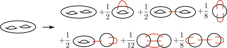
Figure 2: A graphical depiction of the modular transformation of $F_{2}$.

In the following, we will rely very heavily on diagrammatic methods, and we will use the graphical representation shown in Fig. 1 for the different ingredients appearing in the calculations. In this diagrammatic language, the modular transformation of $F_{2}$ can be represented as in Fig. 2, while in Fig. 3 we show the transformation properties of $F_{1}^{\prime}$. The numerical factors in front of each diagram are the symmetry factors of the corresponding diagram, i.e. the number of ways of pinching giving the same diagram, and divided by the order of the automorphism goup. This is the usual symmetry factor of Feynman graphs.

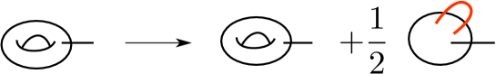
Figure 3: A graphical depiction of the modular transformation of $F_{1}^{\prime}$.

In the context of matrix models, the transformation properties of the $F_{g}$ can be derived from the formalism of [25]. The basic ingredient in this formalism is the transformation property of the Bergmann kernel under a modular transformation,

$${\tilde{B}}(z_{1},z_{2})=B(z_{1},z_{2})+2{\rm i}\pi\omega(z_{1})\,\kappa\,\omega(z_{2}),$$ (3.10)

where $\omega(z)$ is a basis of Abelian holomorphic differentials on $\Sigma$. The $F_{g}$’s of [25] are made of residues of products of Bergmann kernels (see appendix A), namely $F_{g}^{(n)}$ is a sum of residues of products of $3g-3+n$ Bergmann kernels, and multiplied by terms independent of a choice of cycles. Each term of $F_{g}^{(n)}$ is thus represented in [25] by a trivalent diagram, with $3g-3+n$ edges. A modular transformation amounts to cutting (or nor cutting) edges of each diagram in all possible ways (such that all subdiagrams have at least one vertex), and each cut edge is replaced by a factor of $\kappa$. We illustrate these rules in Fig. 4. One has for example

$${\tilde{F}}_{0}^{(4)}=F_{0}^{(4)}+3{\kappa\over 2{\rm i}\pi}(F_{0}^{\prime\prime\prime})^{2},$$ (3.11)

Thus, the modular transformation of $F_{g}^{(n)}$ can be written as a polynomial of degree $3g-3+n$ of $\kappa$. One can show [24], using this property, that one obtains the same diagrammatic calculus as in [1].

Figure 4: A graphical depiction of the modular transformation of $F_{1}^{\prime}$ and $F_{0}^{(4)}$ using the diagrammatic representation of [21, 25]. Each arrowed edge means a propagator $K$ in [25], and each non-arrowed edge means a Bergmann kernel. Each cross at the end of edges, means that we take the ${\cal B}_{i}$ cycle integral corresponding to $\partial/\partial\epsilon_{i}$. For example $\partial F_{1}/\partial\epsilon_{i}=\oint_{z\in{\cal B}_{i}}\,\sum_{j}\mathop{\,\rm Res\,}_{z^{\prime}\to a_{j}}\,K(z,z^{\prime})B(z^{\prime},\bar{z}^{\prime})$. Modular transformations amount to cutting edges in all possible ways such that each subdiagram contains at least one vertex.

3.2 Transformation properties of the theta function

We now study the transformation properties of the $\Theta$-function, and first, we remind the transformation properties of the standard theta function,

$$\tilde{\vartheta}\bigl{[}^{\tilde{\mu}}_{\tilde{\nu}}\bigr{]}(\tilde{\xi}|\tilde{\tau})=\zeta\bigl{[}^{\mu}_{\nu}\bigr{]}(\Gamma)(\gamma\tau+\delta)^{{1\over 2}}\exp\Bigl{[}-\pi{\rm i}\kappa\,\xi^{2}\Bigr{]}\vartheta\bigl{[}^{\mu}_{\nu}\bigr{]}(\xi|\tau),$$ (3.12)

where

$$\tilde{\mu} =\delta\mu-\gamma\nu+{1\over 2}\gamma\delta,$$ (3.13)

$$\tilde{\nu} =-\beta\mu+\alpha\nu+{1\over 2}\alpha\beta,$$

and

$$\zeta\bigl{[}^{\mu}_{\nu}\bigr{]}(\Gamma)=\exp\biggl{\{}-\pi{\rm i}\Bigl{(}\delta\beta\mu^{2}+\gamma\alpha\nu^{2}-2\beta\gamma\mu\nu+\alpha\beta(\delta\mu-\gamma\nu)\Bigr{)}\biggr{\}}\zeta\bigl{[}^{0}_{0}\bigr{]}(\Gamma).$$ (3.14)

Here, $\zeta\bigl{[}^{0}_{0}\bigr{]}(\Gamma)$ is a root of unity which does not depend on the characteristics.

We now deduce an important transformation property of the derivatives of the theta function which will be useful in the following. The derivatives appearing in (2.3) can be computed in terms of the standard theta function by considering

$${1\over(2\pi{\rm i})^{\ell}}\Bigl{(}\partial_{\xi}-N2\pi{\rm i}\epsilon\Bigr{)}^{\ell}\vartheta\bigl{[}^{\mu}_{\nu}\bigr{]}(\xi|\tau),$$ (3.15)

and we are interested on the transformation properties of such quantities under a modular transformation. In evaluating these quantities, the variable $\xi$ is regarded as an independent variable, unrelated to $\epsilon$ and transforming as a modular form of weight $-1$. Only at the very end we set it equal to its true value. Under a modular transformation,

$$\Bigl{(}\partial_{\tilde{\xi}}-N2\pi{\rm i}\tilde{\epsilon}\Bigr{)}^{\ell}\tilde{\vartheta}\bigl{[}^{\tilde{\mu}}_{\tilde{\nu}}\bigr{]}(\tilde{\xi}|\tilde{\tau})={\cal N}\Bigl{(}\partial_{\tilde{\xi}}-N2\pi{\rm i}\tilde{\epsilon}\Bigr{)}^{\ell}\exp\Bigl{[}-\pi{\rm i}\kappa\xi^{2}\Bigr{]}\vartheta\bigl{[}^{\mu}_{\nu}\bigr{]}(\xi|\tau)$$ (3.16)

where ${\cal N}$ does not depend on $\xi$. We now evaluate

$$A_{\ell}(f)=\exp\Bigl{[}\pi{\rm i}\kappa\xi^{2}\Bigr{]}\Bigl{(}\partial_{\tilde{\xi}}-N2\pi{\rm i}\tilde{\epsilon}\Bigr{)}^{\ell}\exp\Bigl{[}-\pi{\rm i}\kappa\xi^{2}\Bigr{]}f(\xi)$$ (3.17)

where $f(\xi)$ is an arbitrary function of $\xi$. We find,

$$A_{\ell}(f)=\Bigl{(}\partial_{\tilde{\xi}}+2\pi{\rm i}\gamma\xi-N2\pi{\rm i}\tilde{\epsilon}\Bigr{)}^{\ell}f(\xi)$$ (3.18)

The operators appearing in the r.h.s. do not commute, and it is easier to consider a generating functional

$$S(x)=\sum_{\ell=0}^{\infty}{A_{\ell}(f)\over\ell!}x^{\ell}={\rm e}^{x(\partial_{\tilde{\xi}}+2\pi{\rm i}\gamma\xi-N2\pi{\rm i}\tilde{\epsilon})}f(\xi).$$ (3.19)

Using the Baker–Campbell–Hausdorff formula, we get

$$S(x)={\rm e}^{x(2\pi{\rm i}\gamma\xi-N2\pi{\rm i}\tilde{\epsilon})}{\rm e}^{-x^{2}\pi{\rm i}\kappa}{\rm e}^{x\partial_{\tilde{\xi}}}f(\xi).$$ (3.20)

After extracting the $\ell$-th power of $x$ in this generating functional, we can already set $\xi$ to its value (2.10). Since

$$2\pi{\rm i}\gamma\xi-N2\pi{\rm i}\tilde{\epsilon}=-(\gamma\tau+\delta)N2\pi{\rm i}\epsilon$$ (3.21)

we finally obtain

$$A_{\ell}(f)=(c\tau+\delta)^{\ell}\sum_{j=0}^{[\ell/2]}(2j-1)!!{\ell\choose 2j}(-2\pi{\rm i}\kappa)^{j}\bigl{(}\partial_{\xi}-N2\pi{\rm i}\epsilon\bigl{)}^{\ell-2j}f(\xi),$$ (3.22)

and this implies the following transformation law for the derivatives of the theta function,

$${1\over\tilde{\vartheta}\bigl{[}^{\tilde{\mu}}_{\tilde{\nu}}\bigr{]}(\tilde{\xi}|\tilde{\tau})}\Bigl{(}{1\over 2\pi{\rm i}}\partial_{\tilde{\xi}}-N\epsilon\Bigr{)}^{\ell}\tilde{\vartheta}\bigl{[}^{\tilde{\mu}}_{\tilde{\nu}}\bigr{]}(\tilde{\xi}|\tilde{\tau})=$$ (3.23)

$${1\over\vartheta\bigl{[}^{\mu}_{\nu}\bigr{]}(\xi|\tau)}(\gamma\tau+\delta)^{\ell}\sum_{j=0}^{[\ell/2]}(2j-1)!!{\ell\choose 2j}\Bigl{(}-{\kappa\over 2\pi{\rm i}}\Bigr{)}^{j}\Bigl{(}{1\over 2\pi{\rm i}}\partial_{\xi}-N\epsilon\Bigr{)}^{\ell-2j}\vartheta\bigl{[}^{\mu}_{\nu}\bigr{]}(\xi|\tau).$$

3.3 Generalization to higher rank

In the higher rank case, the modular group is ${\rm Sp}(2\bar{g},{\mathbb{Z}})$. A modular transformation $\Gamma$ satisfies

$$\Gamma^{\rm T}\Omega\Gamma=\Omega,\qquad\Omega=\begin{pmatrix}0&{\bf 1}\\ -{\bf 1}&0\end{pmatrix},$$ (3.24)

and it can be written as:

$$\Gamma=\begin{pmatrix}A&B\\ C&D\end{pmatrix}$$ (3.25)

where the $\bar{g}\times\bar{g}$ matrices $A$, $B$, $C$, $D$, with integer-valued entries, satisfy

$$A^{\rm T}D-C^{\rm T}B={\bf 1}_{\bar{g}},\,\,\,\ A^{\rm T}C=C^{\rm T}A,\,\,\,\ B^{\rm T}D=D^{\rm T}B.$$ (3.26)

All previous quantities are promoted to vectors and matrices, with obvious generalizations. For example,

$${\tilde{F}}^{\prime}_{0,j} =A_{j}^{~{}k}F^{\prime}_{0,k}+B_{jk}2\pi{\rm i}\epsilon^{k},$$ (3.27)

$$2\pi{\rm i}{\tilde{\epsilon}}^{j} =C^{jk}F^{\prime}_{0,k}+D^{j}_{~{}k}2\pi{\rm i}\epsilon^{k},$$

where summation over repeated indices is understood, and

$${\tilde{\tau}}=(A\tau+B)(C\tau+D)^{-1},\qquad\tilde{\xi}_{i}=\Bigl{[}(C\tau+D)^{-1}\Bigr{]}^{j}_{~{}i}\xi_{j},\quad i=1,\cdots,\bar{g}.$$ (3.28)

The genus zero free energy transforms now as

$$\tilde{F}_{0}=F_{0}+{1\over 2}2\pi{\rm i}\epsilon^{k}(D^{\rm T}B)_{kj}2\pi{\rm i}\epsilon^{j}+{1\over 2}F^{\prime}_{0,k}(C^{\rm T}A)^{kj}F^{\prime}_{0,j}+2\pi{\rm i}\epsilon^{k}(B^{\rm T}C)_{k}^{~{}j}F^{\prime}_{0,j}.$$ (3.29)

The quantity

$$F_{0}-{1\over 2}\epsilon\,F^{\prime}_{0}\equiv F_{0}-{1\over 2}\epsilon^{k}\,F^{\prime}_{0,k}$$ (3.30)

is still invariant, as it can be easily checked. In the following, for general $\bar{g}$, the expressions we used for $\bar{g}=1$ will denote the obvious contraction of indices, as in (3.30) above. We also have the obvious generalization of (3.6),

$$2\pi{\rm i}\epsilon(F_{0}^{\prime}-2\pi{\rm i}\epsilon\tau)\rightarrow 2\pi{\rm i}\epsilon(F_{0}^{\prime}-2\pi{\rm i}\epsilon\tau)-(F_{0}^{\prime}-2\pi{\rm i}\tau\epsilon)\kappa(F_{0}^{\prime}-2\pi{\rm i}\tau\epsilon),$$ (3.31)

where

$$\kappa^{ij}=-\Bigl{[}(C\tau+D)^{-1}C\Bigr{]}^{ij}.$$ (3.32)

This matrix is symmetric, as a consequence of the symplectic properties of $\Gamma$.

The transformation properties of the $F_{g}$ are given by the diagrammatic method explained above. We note that, for $\bar{g}>1$,

$$\tilde{F}_{1}=F_{1}-{1\over 2}\log\,{\rm det}(C\tau+D).$$ (3.33)

Let us now consider the transformation properties of the theta function and its derivatives, in the higher genus case. We have (see for example [5])

$$\tilde{\vartheta}\bigl{[}^{\tilde{\mu}}_{\tilde{\nu}}\bigr{]}(\tilde{\xi}|\tilde{\tau})=\zeta\bigl{[}^{\mu}_{\nu}\bigr{]}(\Gamma)\Bigl{(}{\rm det}(C\tau+D)\Bigr{)}^{{1\over 2}}\exp\Bigl{[}-\pi{\rm i}\xi\kappa\xi\Bigr{]}\vartheta\bigl{[}^{\mu}_{\nu}\bigr{]}(\xi|\tau).$$ (3.34)

In this transformation, the characteristics are given by

$$\tilde{\mu} =D\mu-C\nu+{1\over 2}(CD^{T})_{\rm d},$$ (3.35)

$$\tilde{\nu} =-B\mu+A\nu+{1\over 2}(AB^{T})_{\rm d}.$$

where $(M)_{\rm d}$ denotes a column vector whose entries are the diagonal entries of the matrix $M$. The phase is now given by

$$\zeta\bigl{[}^{\mu}_{\nu}\bigr{]}(\Gamma)=\exp\biggl{\{}-\pi{\rm i}\Bigl{(}\mu D^{T}B\mu+\nu C^{T}A\nu-2\mu B^{T}C\nu+(\mu D^{T}-\nu C^{T})(AB^{T})_{\rm d}\Bigr{)}\biggr{\}}\zeta\bigl{[}^{0}_{0}\bigr{]}(\Gamma).$$ (3.36)

We now consider the derivatives of the theta function. We want to generalize (3.23) and to compute the modular transformation of

$$\Bigl{(}\partial^{j_{1}}-N2\pi{\rm i}\epsilon^{j_{1}}\Bigr{)}\cdots\Bigl{(}\partial^{j_{\ell}}-N2\pi{\rm i}\epsilon^{j_{\ell}}\Bigr{)}\vartheta\bigl{[}^{\mu}_{\nu}\bigr{]}(\xi|\tau),$$ (3.37)

where

$$\partial^{j}={\partial\over\partial\xi_{j}}.$$ (3.38)

Under a modular transformation,

$$\Bigl{(}\tilde{\partial}^{j_{1}}-N2\pi{\rm i}\tilde{\epsilon}^{j_{1}}\Bigr{)}\cdots\Bigl{(}\tilde{\partial}^{j_{\ell}}-N2\pi{\rm i}\tilde{\epsilon}^{j_{\ell}}\Bigr{)}\vartheta\bigl{[}^{\tilde{\mu}}_{\tilde{\nu}}\bigr{]}(\tilde{\xi}|\tilde{\tau})=$$ (3.39)

$${\cal N}\Bigl{(}\tilde{\partial}^{j_{1}}-N2\pi{\rm i}\tilde{\epsilon}^{j_{1}}\Bigr{)}\cdots\Bigl{(}\tilde{\partial}^{j_{\ell}}-N2\pi{\rm i}\tilde{\epsilon}^{j_{\ell}}\Bigr{)}\exp\Bigl{[}-\pi{\rm i}\xi\kappa\xi\Bigr{]}\vartheta\bigl{[}^{\mu}_{\nu}\bigr{]}(\xi|\tau)$$

where ${\cal N}$ is again independent of $\xi$. Since

$$\Bigl{(}\tilde{\partial}^{j}-N2\pi{\rm i}\tilde{\epsilon}^{j}\Bigr{)}\exp\Bigl{[}-\pi{\rm i}\xi\kappa\xi\Bigr{]}=\exp\Bigl{[}-\pi{\rm i}\xi\kappa\xi\Bigr{]}\Bigl{(}\tilde{\partial}^{j}+2\pi{\rm i}C^{jk}\xi_{k}-N2\pi{\rm i}\tilde{\epsilon}^{j}\Bigr{)}$$ (3.40)

we just have to compute

$$A^{j_{1}}\cdots A^{j_{\ell}}\,\vartheta\bigl{[}^{\mu}_{\nu}\bigr{]}(\xi|\tau).$$ (3.41)

where the operator $A^{j}$ is given by

$$A^{j}=(C\tau+D)^{j}_{~{}k}\partial^{k}+2\pi{\rm i}C^{jk}\xi_{k}-N2\pi{\rm i}\tilde{\epsilon}^{j}.$$ (3.42)

As it happened in the $\bar{g}=1$ case, the operators $A^{j_{1}}$, $\cdots$, $A^{j_{\ell}}$ do not commute, since we cannot set $\xi_{k}$ to its value until we have not commuted all the derivatives to the right. Of course, this is precisely the type of computation that Wick’s theorem does. In this context, we define a normal-ordered operator as an operator in which we set

$$\xi_{k}=N\Bigl{(}{F_{0,k}^{\prime}\over 2\pi{\rm i}}-\tau_{kl}\epsilon^{l}\Bigr{)},$$ (3.43)

i.e. we have

$$:A^{j_{1}}\cdots A^{j_{\ell}}:\,=(C\tau+D)^{j_{1}}_{~{}k_{1}}\cdots(C\tau+D)^{j_{\ell}}_{~{}k_{\ell}}(\partial^{k_{1}}-N2\pi{\rm i}\epsilon^{k_{1}})\cdots(\partial^{k_{\ell}}-N2\pi{\rm i}\epsilon^{k_{\ell}}).$$ (3.44)

The contraction is given by

$$\langle A^{j}A^{k}\rangle=2\pi{\rm i}C^{jk}=(C\tau+D)^{j}_{~{}l}(-2\pi{\rm i}\kappa)^{lk}.$$ (3.45)

We can now apply Wick’s theorem to write the operator in (3.41) as a sum of normal-ordered operators. In the end we obtain

$${1\over\tilde{\vartheta}\bigl{[}^{\tilde{\mu}}_{\tilde{\nu}}\bigr{]}(\tilde{\xi}|\tilde{\tau})}\Bigl{(}{1\over 2\pi{\rm i}}\tilde{\partial}^{p_{1}}-N\tilde{\epsilon}^{p_{1}}\Bigr{)}\cdots\Bigl{(}{1\over 2\pi{\rm i}}\tilde{\partial}^{p_{\ell}}-N\tilde{\epsilon}^{p_{\ell}}\Bigr{)}\vartheta\bigl{[}^{\tilde{\mu}}_{\tilde{\nu}}\bigr{]}(\tilde{\xi}|\tilde{\tau})=$$ (3.46)

$${1\over\vartheta\bigl{[}^{\mu}_{\nu}\bigr{]}(\xi|\tau)}(C\tau+D)^{p_{1}}_{~{}q_{1}}\cdots(C\tau+D)^{p_{\ell}}_{~{}q_{\ell}}\sum_{j=0}^{[\ell/2]}\sum_{\sigma}\Bigl{(}-{\kappa\over 2\pi{\rm i}}\Bigr{)}^{q_{\sigma(1)}q_{\sigma(2)}}\cdots\Bigl{(}-{\kappa\over 2\pi{\rm i}}\Bigr{)}^{q_{\sigma(2j-1)}q_{\sigma(2j)}}$$

$$\Bigl{(}{1\over 2\pi{\rm i}}\partial^{q_{\sigma(2j+1)}}-N\epsilon^{q_{\sigma(2j+1)}}\Bigr{)}\cdots\Bigl{(}{1\over 2\pi{\rm i}}\partial^{q_{\sigma(\ell)}}-N\epsilon^{q_{\sigma(\ell)}}\Bigr{)}\vartheta\bigl{[}^{\mu}_{\nu}\bigr{]}(\xi|\tau).$$

In the r.h.s., the first sum is over the number $j$ of contractions. The second sum is over all possible ways of performing the contractions, and $\sigma$ denotes the permutation of the indices $1,\cdots,\ell$ associated to a given contraction (note that not all possible permutations appear). (3.46) is the generalization of (3.23) to the multi-index case. Indeed, the combinatorial factor in the r.h.s. of (3.23) is simply the number of possible ways of performing $j$ contractions in $\ell$ terms: the combinatorial number accounts for the choices of $2j$ legs to be contracted among $\ell$ legs in total, and $(2j-1)!!$ is the number of possible pairings of the $2j$ legs.

Of course, the easiest way of keeping track of combinatorial formulae like the above is by means of a graphical representation. Using the building blocks shown in Fig. 1, the equation (3.46) might be represented as in Fig. 5, where some simple examples are also shown.

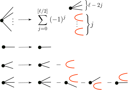
Figure 5: The first line gives a graphical representation of (3.46), while the next lines exemplify it for $\ell=1,2,3$. Notices that the edges are labeled, and when summing over all possible contractions we have to take this labeling into account, as shown in the last example.

3.4 Transformation properties of the nonperturbative partition function

We will now study in detail the transformation properties of the nonperturbative partition function (2.3). We rewrite (2.3) as:

$$Z_{\Sigma}(\mu,\nu;\epsilon) ={{\rm e}^{N^{2}F_{0}+F_{1}}}\,\Theta_{\mu,\nu}\,\biggl{\{}1+\sum_{j=1}^{\infty}N^{-j}\,Z_{j}(\mu,\nu;\epsilon)\biggr{\}}$$ (3.47)

$$={{\rm e}^{N^{2}F_{0}+F_{1}}}\,\Theta_{\mu,\nu}\,\biggl{\{}1+{1\over N}\Bigl{(}{\Theta^{\prime}_{\mu,\nu}\over\Theta_{\mu,\nu}}F_{1}^{\prime}+{1\over 6}{\Theta_{\mu,\nu}^{\prime\prime\prime}\over\Theta_{\mu,\nu}}\,F_{0}^{\prime\prime\prime}\Bigr{)}$$

$$+{1\over N^{2}}\Bigl{(}F_{2}+{1\over 2}{\Theta^{\prime\prime}_{\mu,\nu}\over\Theta_{\mu,\nu}}F_{1}^{\prime\prime}+{1\over 2}{\Theta^{\prime\prime}_{\mu,\nu}\over\Theta_{\mu,\nu}}F_{1}^{\prime 2}+{1\over 24}{\Theta^{(4)}_{\mu,\nu}\over\Theta_{\mu,\nu}}F_{0}^{\prime\prime\prime\prime}+{1\over 6}{\Theta^{(4)}_{\mu,\nu}\over\Theta_{\mu,\nu}}F_{0}^{\prime\prime\prime}F^{\prime}_{1}+{1\over 72}{\Theta^{(6)}_{\mu,\nu}\over\Theta_{\mu,\nu}}(F_{0}^{\prime\prime\prime})^{2}\Bigr{)}$$

$$+\dots\biggr{\}}$$

i.e. $Z_{j}$ is the sum of all terms contributing to order $N^{-j}$.

We first study the transformation properties of the leading term ${{\rm e}^{N^{2}F_{0}+F_{1}}}\,\Theta_{\mu,\nu}$. To do this, we use the relation (2.9) to write

$${\rm e}^{N^{2}F_{0}}\Theta_{\mu,\nu}=\exp\biggl{[}N^{2}\Bigl{(}F_{0}-\epsilon F_{0}^{\prime}-{1\over 2}\epsilon^{2}F_{0}^{\prime\prime}\Bigr{)}\biggr{]}\vartheta\bigl{[}^{\mu}_{\nu}\bigr{]}(\xi|\tau).$$ (3.48)

In order to study the transformation properties of this quantity, we have to study the transformation properties of

$$\Xi=F_{0}-\epsilon F_{0}^{\prime}-{1\over 2}\epsilon^{2}F_{0}^{\prime\prime}=F_{0}-{1\over 2}\epsilon F_{0}^{\prime}-{1\over 2}\epsilon\Bigl{(}F^{\prime}_{0}-2\pi{\rm i}\epsilon\tau\Bigr{)}.$$ (3.49)

Using (3.31) and the invariance of (3.30), one finds that

$$\widetilde{\Xi}=\Xi+\pi{\rm i}\biggl{(}{F^{\prime}_{0}\over 2\pi{\rm i}}-\tau\epsilon\biggr{)}\kappa\biggl{(}{F^{\prime}_{0}\over 2\pi{\rm i}}-\tau\epsilon\biggr{)},$$ (3.50)

therefore the shift in $\Xi$ exactly compensates the $\xi$ dependent exponent in the transformation (3.34) and we find,

$${\rm e}^{N^{2}\tilde{F}_{0}}\widetilde{\Theta}_{\tilde{\mu},\tilde{\nu}}(\tilde{u},\tilde{\tau})=\zeta\bigl{[}^{\mu}_{\nu}\bigr{]}(\Gamma)\bigl{(}{\rm det}(C\tau+D)\bigr{)}^{{1\over 2}}{\rm e}^{N^{2}F_{0}}\Theta_{\mu,\nu}(u,\tau).$$ (3.51)

It follows immediately from (3.33) that

$${\rm e}^{N^{2}\tilde{F}_{0}+\tilde{F}_{1}}\widetilde{\Theta}_{\tilde{\mu},\tilde{\nu}}(\tilde{u},\tilde{\tau})=\zeta\bigl{[}^{\mu}_{\nu}\bigr{]}(\Gamma)\,{\rm e}^{N^{2}F_{0}+F_{1}}\Theta_{\mu,\nu}(u,\tau)$$ (3.52)

under a general ${\rm Sp}(2\bar{g},{\mathbb{Z}})$ transformation. This proves (1.2) to leading order in $N$.

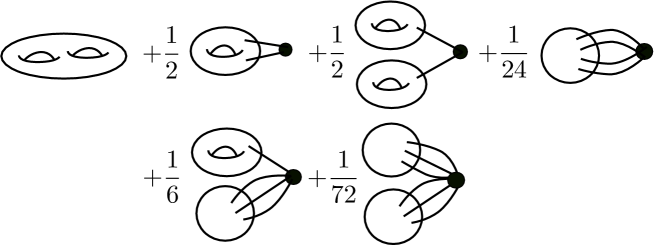
Figure 6: Graphic representation of $Z_{2}$, the term in $1/N^{2}$ in the expansion of $Z$.

Our goal is now to prove that each $Z_{j}$ is itself modular invariant, up to the change of characteristics (3.35).

$Z_{j}$ is given by a sum, and each term in this sum is the product of a derivative of $\Theta$, with a product of a certain number of derivatives of $F_{h}$’s corresponding to the stable degeneracy of (possibly non-connected) surfaces with Euler characteristics $\chi=-j$. Notice that, in each term, the total number of derivatives acting on the $F_{h}$ equals the number of derivatives acting on $\Theta$. As shown in Fig. 1, $\Theta^{(n)}/\Theta$, the $n^{\rm th}$ derivative of $\Theta$, is depicted as a black dot with $n$ legs, while $F_{h}^{(n)}$ is depicted as a Riemann surface of genus $h$ with $n$ marked points. Each term in $Z_{j}$ can thus be depicted as a set of stable Riemann surfaces with marked points linked to the legs of the $\Theta^{(n)}/\Theta$ term. Notice that there can be disconnected terms corresponding to $F_{h}^{(n)}$ with $n=0$. Also, each term has a symmetry factor, which is, as usual in Feynmann graphs, the number of possible pairings of indices, divided by the group order $k!\,l_{1}!\dots l_{k}!$. As an example, we depict $Z_{2}$ in Fig. 6.

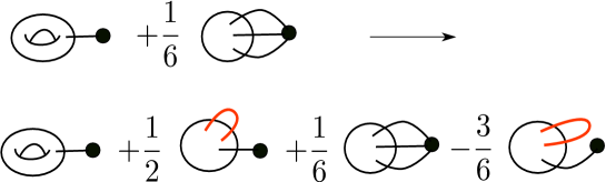
Figure 7: Graphic proof of the modular invariance of the term $Z_{1}$ of order $1/N$ in the expansion of $Z$.

Under a modular transformation, each $F_{h}^{(n)}$ transforms into a sum of stable degenerated surfaces, with a factor $\kappa/(2\pi{\rm i})$ for each degenerated cycle. As shown in (3.46) (and as illustrated in Fig. 5) the $\Theta^{(n)}/\Theta$ term transforms into a sum of $\Theta^{(k)}/\Theta$ where $(n-k)/2$ legs are replaced by a $-\kappa/(2\pi{\rm i})$ in all possible ways (with a change of characteristics as (3.35). The factors of $C\tau+D$ appearing in (3.46) cancel against the factors of $(C\tau+D)^{-1}$ coming from the derivatives of the $F_{h}$’s.

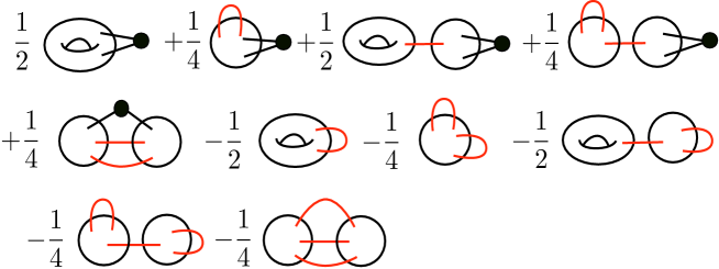
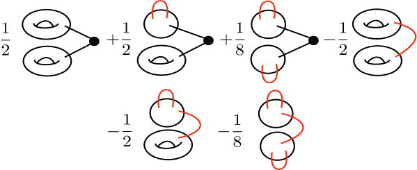
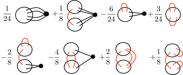
Figure 8: Modular transformation of the second, third and fourth graphs in Fig. 6 .

In the end, ${\tilde{Z}}_{j}$ is a sum of terms, each of them is the product of a $\Theta^{(k)}/\Theta$, with a certain number of $F_{h_{i}}^{(n_{i})}$’s, and a certain number of $\kappa$ propagators. Each propagator can be obtained in two ways, either from a degeneracy of a $F_{h}^{(n)}$, with a factor $+(2{\rm i}\pi)^{-1}$, or from a term $\Theta^{(k)}/\Theta$, with a factor $-(2{\rm i}\pi)^{-1}$. Also, the symmetry factors are counting the number of possible pairings corresponding to a given diagramm, and are the same whether obtained from the modular transformation of $\Theta^{(k)}/\Theta$, or from the modular transformation of $F_{h_{i}}^{(n_{i})}$’s. Therefore, the total contribution of each $\kappa$ propagator is $0$. This shows that

$${\tilde{Z}}_{j}(\tilde{\mu},\tilde{\nu})=Z_{j}(\mu,\nu)$$ (3.53)

therefore we have proved that

$$\tilde{Z}_{\Sigma}(\tilde{\mu},\tilde{\nu};\tilde{\epsilon})=\zeta\bigl{[}^{\mu}_{\nu}\bigr{]}(\Gamma)\,\,Z_{\Sigma}(\mu,\nu;\epsilon)$$ (3.54)

We illustrate the proof by the examples of $Z_{1}$ and $Z_{2}$. In the case of $Z_{1}$, we know from Fig. 3 the transformation rule of $F_{1}^{\prime}$, and from Fig. 5 we know the transformation properties of $\Theta^{\prime}/\Theta$ and $\Theta^{\prime\prime\prime}/\Theta$. Since $F_{0}^{\prime\prime\prime}$ transforms as a modular form of weight $-3$ (i.e., there are no shifts involved) and it is completely symmetric in its indices, we immediately obtain the graphic proof of modular invariance of $Z_{1}$ depicted in Fig. 7.

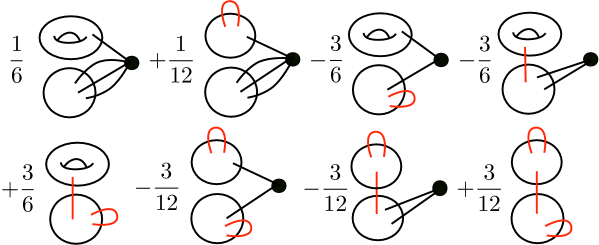
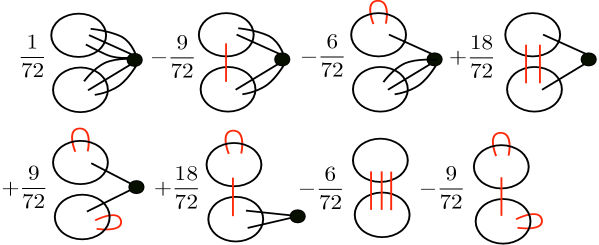
Figure 9: Modular transformation of the fifth and sixth graphs in Fig. 6 .

The terms appearing in $Z_{2}$ were depicted graphically in Fig. 6. The modular transformation of $F_{2}$, which is the first term, was shown in Fig. 2. The modular transformation of the rest of the graphs in Fig. 6 is shown in Fig. 8 and Fig. 9. One can check that all the graphs generated on top of the original ones (i.e., all the shifts generated by the modular transformation, i.e. all graphs containing propagators $\kappa$) eventually cancel, and $Z_{2}$ remains invariant up to the change of characteristics. For example, the second graph in the first line of Fig. 8 cancels against the third graph in the sixth line of the same figure, while the third graph in the first line of Fig. 8 cancels against the fourth graph in the first line of Fig. 9. In a similar manner, all graphs in Fig. 2, Fig. 8 and Fig. 9 containing propagators eventually cancel.

3.5 Background independence

We now show that the non-perturbative partition function is background independent, i.e. it does not depend on the background filling fraction $\epsilon$. This is not surprising, because this is how it was first constructed in [22].

Let

$$\hat{Z}(\eta)={{\rm e}^{\sum_{g\geq 0}N^{2-2g}F_{g}(\eta)}}$$ (3.55)

be the perturbative partition function. We may Taylor expand it near an arbitrary background filling fraction $\epsilon$:

$$\hat{Z}(\eta) =\sum_{j}{1\over j!}(\eta-\epsilon)^{j}\,\,\hat{Z}^{(j)}(\epsilon)$$ (3.56)

$$={{\rm e}^{N^{2}(F_{0}+(\eta-\epsilon)F^{\prime}_{0}+{1\over 2}(\eta-\epsilon)^{2}F^{\prime\prime}_{0})}}\,{{\rm e}^{F_{1}}}\,\,{{\rm e}^{\sum_{g\geq 2}N^{2-2g}F_{g}}}$$

$$\cdot\sum_{k}\sum_{l_{i}>0}\sum_{h_{i}>1-{l_{i}\over 2}}{N^{\sum_{i}(2-2h_{i})}\over k!l_{1}!\,\dots\,l_{k}!}{F_{h_{1}}^{(l_{1})}}\dots F_{h_{k}}^{(l_{k})}\,\,(\eta-\epsilon)^{\sum_{i}l_{i}}.$$

Therefore we recognize that the nonperturbative partition function (2.3) is the Taylor expansion of

$$Z_{\Sigma}(\mu,\nu;\epsilon)=\sum_{{\bf n}\in{\mathbb{Z}}^{\bar{g}}}\hat{Z}\Bigl{(}{n+\mu\over N}\Bigr{)}\,\,{{\rm e}^{2{\rm i}\pi n\nu}}.$$ (3.57)

The right hand side of this expression is clearly independent of $\epsilon$:

$$Z_{\Sigma}(\mu,\nu;\epsilon)=Z_{\Sigma}(\mu,\nu;\epsilon^{\prime})$$ (3.58)

and thus $Z_{\Sigma}(\mu,\nu;\epsilon)=Z_{\Sigma}(\mu,\nu)$ is background independent.

We can see more explicitly that $Z_{\Sigma}(\mu,\nu;\epsilon)$ is locally constant, as a function of $\epsilon$, by showing that ${\rm d}Z/{\rm d}\epsilon=0$. Let us first define

$$\Theta_{k}:={{\rm e}^{N^{2}F_{0}+F_{1}}}\,\,\left.{{\rm d}^{k}\over{\rm d}u^{k}}\Theta\right|_{u=NF^{\prime}_{0}}.$$ (3.59)

In this equation and the following ones we will not indicate the characteristics of the theta function in order to simplify the notation. Using (3.59) we can write

$$Z_{\Sigma}(\mu,\nu;\epsilon) =\Theta_{0}+{1\over N}\Bigl{(}F^{\prime}_{1}\Theta_{1}+{F_{0}^{\prime\prime\prime}\over 6}\Theta_{3}\Bigr{)}$$ (3.60)

$$+{1\over N^{2}}\Bigl{(}F_{2}\Theta_{0}+{F_{1}^{\prime\prime}\over 2}\Theta_{2}+{F_{1}^{\prime 2}\over 2}\Theta_{2}+{F_{0}^{\prime\prime\prime\prime}\over 24}\Theta_{4}+{F_{0}^{\prime\prime\prime}F_{1}^{\prime}\over 6}\Theta_{4}+{F_{0}^{\prime\prime\prime 2}\over 72}\Theta_{6}\Bigr{)}+\dots$$

It is easy to compute that (where ${}^{\prime}={\rm d}/{\rm d}\epsilon$)

$$\Theta_{k}^{\prime}=F^{\prime}_{1}\Theta_{k}-kN\Theta_{k-1}+{F_{0}^{\prime\prime\prime}\over 2}\Theta_{k+2}$$ (3.61)

and, as a formal power series, we have that

$${{\rm d}Z_{\Sigma}\over{\rm d}\epsilon} =\Theta_{0}^{\prime}+{1\over N}\Bigl{(}F^{\prime\prime}_{1}\Theta_{1}+F^{\prime}_{1}\Theta^{\prime}_{1}+{F_{0}^{\prime\prime\prime\prime}\over 6}\Theta_{3}+{F_{0}^{\prime\prime\prime}\over 6}\Theta_{3}^{\prime}\Bigr{)}$$ (3.62)

$$+{1\over N^{2}}\Bigl{(}F_{2}^{\prime}\Theta_{0}+F_{2}\Theta_{0}^{\prime}+{F_{1}^{\prime\prime\prime}\over 2}\Theta_{2}+{F_{1}^{\prime\prime}\over 2}\Theta_{2}^{\prime}+{F_{1}^{\prime 2}\over 2}\Theta_{2}^{\prime}+F_{1}^{\prime}F_{1}^{\prime\prime}\Theta_{2}+{F_{0}^{(5)}\over 24}\Theta_{4}$$

$$+{F_{0}^{\prime\prime\prime\prime}\over 24}\Theta_{4}^{\prime}+{F_{0}^{\prime\prime\prime}F_{1}^{\prime\prime}\over 6}\Theta_{4}+{F_{0}^{\prime\prime\prime\prime}F_{1}^{\prime}\over 6}\Theta_{4}+{F_{0}^{\prime\prime\prime}F_{1}^{\prime}\over 6}\Theta_{4}^{\prime}+{F_{0}^{\prime\prime\prime}F_{0}^{\prime\prime\prime\prime}\over 36}\Theta_{6}+{F_{0}^{\prime\prime\prime 2}\over 72}\Theta_{6}^{\prime}\Bigr{)}+\cdots$$

$$=F^{\prime}_{1}\Theta_{0}+{F_{0}^{\prime\prime\prime}\over 2}\Theta_{2}+{1\over N}\Bigl{(}F^{\prime\prime}_{1}\Theta_{1}+F^{\prime}_{1}(F^{\prime}_{1}\Theta_{1}-N\Theta_{0}+{F_{0}^{\prime\prime\prime}\over 2}\Theta_{3})+{F_{0}^{\prime\prime\prime\prime}\over 6}\Theta_{3}$$

$$+{F_{0}^{\prime\prime\prime}\over 6}(F^{\prime}_{1}\Theta_{3}-3N\Theta_{2}+{F_{0}^{\prime\prime\prime}\over 2}\Theta_{5})\Bigr{)}$$

$$+{1\over N^{2}}\Bigl{(}F_{2}^{\prime}\Theta_{0}+F_{2}(F^{\prime}_{1}\Theta_{0}+{F_{0}^{\prime\prime\prime}\over 2}\Theta_{2})+{F_{1}^{\prime\prime\prime}\over 2}\Theta_{2}+{F_{1}^{\prime\prime}\over 2}(F^{\prime}_{1}\Theta_{2}-2N\Theta_{1}+{F_{0}^{\prime\prime\prime}\over 2}\Theta_{4})$$

$$+{F_{1}^{\prime 2}\over 2}(F^{\prime}_{1}\Theta_{2}-2N\Theta_{1}+{F_{0}^{\prime\prime\prime}\over 2}\Theta_{4})+F_{1}^{\prime}F_{1}^{\prime\prime}\Theta_{2}+{F_{0}^{(5)}\over 24}\Theta_{4}$$

$$+{F_{0}^{\prime\prime\prime\prime}\over 24}(F^{\prime}_{1}\Theta_{4}-4N\Theta_{3}+{F_{0}^{\prime\prime\prime}\over 2}\Theta_{6})$$

$$+{F_{0}^{\prime\prime\prime}F_{1}^{\prime\prime}\over 6}\Theta_{4}+{F_{0}^{\prime\prime\prime\prime}F_{1}^{\prime}\over 6}\Theta_{4}+{F_{0}^{\prime\prime\prime}F_{1}^{\prime}\over 6}(F^{\prime}_{1}\Theta_{4}-4N\Theta_{3}+{F_{0}^{\prime\prime\prime}\over 2}\Theta_{6})$$

$$+{F_{0}^{\prime\prime\prime}F_{0}^{\prime\prime\prime\prime}\over 36}\Theta_{6}+{F_{0}^{\prime\prime\prime 2}\over 72}(F^{\prime}_{1}\Theta_{6}-6N\Theta_{5}+{F_{0}^{\prime\prime\prime}\over 2}\Theta_{8})\Bigr{)}+\cdots$$

One easily checks that the term of order $N^{0}$ in this series is

$$F^{\prime}_{1}\Theta_{0}+{F_{0}^{\prime\prime\prime}\over 2}\Theta_{2}+{1\over N}(F^{\prime}_{1}(-N\Theta_{0})+{F_{0}^{\prime\prime\prime}\over 6}(-3N\Theta_{2}))=0.$$ (3.63)

The term of order $1/N$ is

$$F^{\prime\prime}_{1}\Theta_{1}+F^{\prime}_{1}(F^{\prime}_{1}\Theta_{1}+{F_{0}^{\prime\prime\prime}\over 2}\Theta_{3})+{F_{0}^{\prime\prime\prime\prime}\over 6}\Theta_{3}+{F_{0}^{\prime\prime\prime}\over 6}(F^{\prime}_{1}\Theta_{3}+{F_{0}^{\prime\prime\prime}\over 2}\Theta_{5})$$ (3.64)

$$+{1\over N}\Bigl{(}{F_{1}^{\prime\prime}\over 2}(-2N\Theta_{1})+{F_{1}^{\prime 2}\over 2}(-2N\Theta_{1})+{F_{0}^{\prime\prime\prime\prime}\over 24}(-4N\Theta_{3})+{F_{0}^{\prime\prime\prime}F_{1}^{\prime}\over 6}(-4N\Theta_{3})+{F_{0}^{\prime\prime\prime 2}\over 72}(-6N\Theta_{5})\Bigr{)}$$

$$=0.$$

This shows that, at this order in the $1/N$ expansion, $Z_{\Sigma}(\mu,\nu;\epsilon)$ is locally constant as a function of the filling fractions:

$${{\rm d}Z_{\Sigma}\over{\rm d}\epsilon}=0.$$ (3.65)

The generalization at all orders can be done by using the graphical techniques developed above.

4 Matrix models and sums over filling fractions

Let us briefly summarize [22], which is just an improved version of [11], to explain the origin of the definition (2.3) for the non-perturbative partition function.

4.1 Matrix integrals and domains of integration

A matrix integral is typically an integral of the form:

$$Z={1\over N!}\,\int{\rm d}x_{1}\dots\rm dx_{N}\,\,\prod_{i>j}(x_{i}-x_{j})^{2}\,\,\prod_{i}{{\rm e}^{-NV(x_{i})}}$$ (4.66)

where we have not written the integration domain. For any choice of integration domain, $Z$ satisfies the same loop equations (i.e. Schwinger-Dyson equations), as long as there is no boundary term when one integrates by parts.

For example, one may consider the matrix integral over $H_{N}(\gamma)$ (the set of normal matrices with eigenvalues constrained on a path $\gamma$):

$$Z(\gamma)=\int_{H_{N}(\gamma)}{\rm d}M\,{{\rm e}^{-N{\,\rm Tr}\>V(M)}}={1\over N!}\,\int_{\gamma^{N}}{\rm d}x_{1}\dots\rm dx_{N}\,\,\prod_{i>j}(x_{i}-x_{j})^{2}\,\,\prod_{i}{{\rm e}^{-NV(x_{i})}}.$$ (4.67)

This integral depends only on a choice of path $\gamma$, and it has a $U(N)$ invariance.

One may also consider the following integral where $N=\sum_{i}n_{i}$:

$$\hat{Z}_{n_{1},\dots,n_{k}}={1\over\prod_{i}n_{i}!}\,\int_{\gamma_{1}^{n_{1}}\times\dots\times\gamma_{k}^{n_{k}}}{\rm d}x_{1}\dots\rm dx_{N}\,\,\prod_{i>j}(x_{i}-x_{j})^{2}\,\,\prod_{i}{{\rm e}^{-NV(x_{i})}}.$$ (4.68)

The parameters $\epsilon_{i}=n_{i}/N$ are called the filling fractions, because they represent the fraction of the eigenvalues on each path $\gamma_{i}$. This integral depends on a choice of filling fractions, called “background filling fraction”, and it only has a $U(n_{1})\times U(n_{2})\times\dots\times U(n_{k})$ invariance.

One may also write a path in different ways, and for instance if $\gamma_{1},\dots,\gamma_{k}$ form a homological basis of paths on which integrals of type (4.66) can be performed [10], then any path $\gamma$ can be decomposed on such a basis:

$$\gamma=\sum_{i}c_{i}\gamma_{i}$$ (4.69)

and one may relate $Z(\gamma)$ and $\hat{Z}_{n_{1},\dots,n_{k}}$:

$$Z(\gamma)=\sum_{\sum_{i}n_{i}=N}\,\prod_{i}c_{i}^{n_{i}}\,\,\hat{Z}_{n_{1},\dots,n_{k}}.$$ (4.70)

Since not all $n_{i}$ are independent, we can fix the overall normalization of $Z(\gamma)$ by setting $c_{1}=1$. One may also study changes of paths in $\hat{Z}_{n_{1},\dots,n_{k}}$.

4.2 Topological perturbative expansion

For some special choices of $\gamma$, or alternatively for some special choices of the basis $\gamma_{1},\dots,\gamma_{k}$ and some special choices of filling fractions $n_{1},\dots,n_{k}$, it may happen that $\ln{Z}$, or $\ln{\hat{Z}}$ have a perturbative large $N$ expansion:

$$\ln{\hat{Z}_{n_{1},\dots,n_{k}}}=\sum_{g=0}^{\infty}N^{2-2g}\,F_{g}.$$ (4.71)

If such $F_{g}$’s exist, then Schwinger-Dyson equations imply [21, 14] that they coincide with the symplectic invariants defined in [25], for some spectral curve. This matrix model spectral curve is the so called “equilibrium density” of eigenvalues.

However, for most paths $\gamma$, or for arbitrary choices of the basis $\gamma_{1},\dots,\gamma_{k}$ and arbitrary choices of filling fractions $n_{1},\dots,n_{k}$, matrix integrals have no perturbative large $N$ expansion.

We conjecture (which is proved for special cases, for instance for the one-matrix model [9]), that given a potential $V$, and given $n_{1},\dots,n_{k}$, there always exists a “good” basis of paths $\gamma_{1},\dots,\gamma_{k}$, such that $\hat{Z}_{n_{1},\dots,n_{k}}$ has a topological expansion of the form (4.71). In some sense, this “good” basis of paths is made of the steepest descent contours for the integral (4.66).

4.3 Summation over filling fractions

Using (4.70)

$$Z(\gamma)=\sum_{\sum_{i}n_{i}=N}\,\prod_{i}c_{i}^{n_{i}}\,\,\hat{Z}_{n_{1},\dots,n_{k}}$$ (4.72)

and the fact that each $\hat{Z}_{n_{1},\dots,n_{k}}$ has a perturbative expansion of type (4.71), we can find the asymptotic expansion of $Z(\gamma)$ as a combination of $\hat{Z}_{n_{1},\dots,n_{k}}$ after summation over the filling fractions $n_{i}$. This goes as follows.

For various matrix models, including the 1-matrix model, the 2-matrix model, the chain of matrices, and matrix models with external fields, the coefficients $F_{g}$ in (4.71) have been computed in [14, 15, 26, 25], and are the symplectic invariants of [25]. They happen to be analytic in the filling fraction variables $n_{i}/N$, and thus they can be Taylor expanded near an arbitrary background value $\epsilon_{i}$:

$$N^{2-2g}\,F_{g}(n_{i}/N)=\sum_{k}{N^{2-2g-k}\,(n_{i}-N\epsilon_{i})^{k}\over k!}\,F_{g}^{(k)}(\epsilon_{i}).$$ (4.73)

The only terms with non-negative powers of $N$ correspond to $N^{2}F_{0}+F_{1}+(n-N\epsilon)NF^{\prime}_{0}+{1\over 2}(n-N\epsilon)^{2}F_{0}^{\prime\prime}$. All the other terms have negative power of $N$, and thus can be expanded at large $N$, so that:

$$\hat{Z}_{n_{1},\dots,n_{k}} \sim{{\rm e}^{N^{2}F_{0}+F_{1}+\sum_{g\geq 2}N^{2-2g}F_{g}}}\,\,$$ (4.74)

$$\sum_{k}\sum_{l_{i}>0}\sum_{h_{i}>1-{l_{i}\over 2}}{N^{\sum_{i}(2-2h_{i}-l_{i})}\over k!l_{1}!\,\dots\,l_{k}!}\,\,\,F_{h_{1}}^{(l_{1})}\dots F_{h_{k}}^{(l_{k})}\,\,(n-N\epsilon)^{\sum_{i}l_{i}}\,\,{{\rm e}^{(n-N\epsilon)NF^{\prime}_{0}+{1\over 2}(n-N\epsilon)^{2}F_{0}^{\prime\prime}}}.$$

The sum over filling fractions (4.72) generates the non-perturbative partition function of [22], i.e. (2.3), under the identification:

$$\mu_{i}=0,\qquad c_{i}={{\rm e}^{2{\rm i}\pi\nu_{i}}}.$$ (4.75)

This shows that the choice of a characteristic $(\mu,\nu)$ is related to a choice of integration contour $\gamma$ for the matrix integral (see Fig. 10).

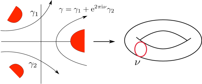
Figure 10: A choice of integration path for the matrix integral determines a choice of characteristic in the spectral curve, corresponding to A-cycles. We illustrate this correspondence in this figure for the case of the cubic matrix model, with a spectral curve of genus one. A typical path of integration for the eigenvalues is $\gamma=\gamma_{1}+{{\rm e}^{2{\rm i}\pi\nu}}\gamma_{2}$ and corresponds to a characteristic $(0,\nu)$.

This simplified description of the origin of the non-perturbative partition function for matrix models seems to involve only characteristics of type $(0,\nu)$, and not all characteristics $(\mu,\nu)$.

However, one should keep in mind that a “good basis of paths” $\gamma_{1},\dots,\gamma_{k}$ is not unique. Changes of basis correspond to modular transformations, and basis can be more complicated than what naive intuition seems to show. In the “naive” picture, it is often thought that, in the large $N$ limit of mutlticut matrix integrals, eigenvalues tend to localize along disconnected segments called “cuts”. In this case, there is a natural choice of $A$-cycles, as contours surrounding the cuts (see Fig. 11, left).

   

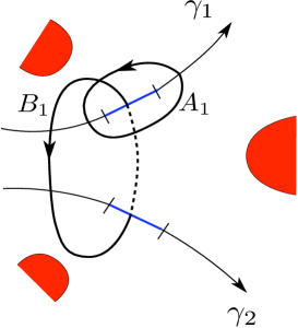
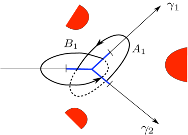
Figure 11: On the left we show a situation in which there is a natural choice of $A$-cycle surrounding the cut along the path $\gamma_{1}$. However, in some situations the eigenvalues might localize on tree structures, as shown in the figure on the right.

But in general, it is well known [17, 9] that, in the large $N$ limit of multicut matrix integrals, eigenvalues tend to localize along forests of 3-valent trees rather than union of segments (see Fig. 11, right). In that case, there is no natural distinction between $A$-cycles and $B$-cycles, and maybe in such tree structures one could probably interpret the general characteristics $(\mu,\nu)$ with $\mu\neq 0$.

4.4 Remarks on background independence

First, notice that we have chosen to perform a Taylor expansion near an arbitrary background filling fraction $\epsilon$, although the partition function $Z(\gamma)$ is independent of $\epsilon$. We clearly have background independence.

Also, we have used the existence of a good basis $\gamma_{1},\dots,\gamma_{k}$. However, such a good basis is not unique, and one may perform changes of basis. Such changes of basis are equivalent to symplectic changes of cycles on the spectral curve. The fact that $Z(\gamma)$ depends intrinsically on $\gamma$, and not on a choice of basis on which $\gamma$ is decomposed as in (4.69), is a hint towards modular invariance.

Finally, we notice that a choice of background leads to a breaking of the original, unitary $U(N)$ symmetry of the matrix integral down to a subgroup $U(n_{1})\times\cdots\times U(n_{k})$. Therefore, the restoration of modular invariance and background independence by non-perturbative corrections seems to be deeply related to the restoration of the $U(N)$ symmetry.

5 The nonperturbative partition function for topological strings

5.1 Topological strings, matrix models and spectral curves

In [20], Dijkgraaf and Vafa showed that the type B topological string, on certain Calabi-Yau (CY) geometries, is equivalent to a Hermitian matrix model with polynomial potential $V(x)$ (see [38] for a review). These target geometries are deformed singularities of the form

$$uv=H(x,y)$$ (5.1)

where $x,y,u,v\in{\mathbb{C}}$ and

$$H(x,y)=y^{2}-V^{\prime 2}(x)-f(x).$$ (5.2)

The nontrivial information about this geometry turns out to be encoded in the Riemann surface $\Sigma$ described by $H(x,y)=0$. An important insight of the analysis of Dijkgraaf and Vafa is that $\Sigma$ is precisely the spectral curve of the corresponding Hermitian matrix model, providing in this way a beautiful example in which the master field of the $1/N$ expansion generates the target geometry of a string theory.

More recently, the correspondence between matrix models/spectral curves and topological strings was extended to toric CY threefolds [39, 12]. This class of examples is very interesting since (in contrast to the geometries considered in [20]) they have mirror geometries. The mirrors are described by an equation of the form (5.1), but where the variables $x,y$ now belong to ${\mathbb{C}}^{*}$, and again the nontrivial part of the geometry reduces to a Riemann surface $\Sigma$ described by $H(x,y)=0$. In [25] it was shown that, given any algebraic curve, not necessarily coming from a matrix model, one can compute a set of “open” and “closed” amplitudes. When the curve is the spectral curve of a matrix model, these amplitudes reproduce the $1/N$ expansion of correlators and free energies, respectively. However, the construction is valid for any spectral curve. The proposal of [39, 12] is to regard the Riemann surface $H(x,y)=0$ appearing in (5.1) as a spectral curve in the general sense of [25], and to identify the open and closed string amplitudes of the B–model with the open and closed amplitudes constructed in [25] purely in terms of data of the spectral curves. Therefore, for this more general class of examples, we rather have a correspondence between the type B topological string amplitudes on the mirror of a toric manifold, and the amplitudes associated to a spectral curve defined in [25].

For certain backgrounds it is however still possible to provide a matrix integral representation. In the case of local curves, i.e. manifolds of the form

$$X_{p}={\cal O}(p)\oplus{\cal O}(-p-2)\rightarrow{\mathbb{P}}^{1}$$ (5.3)

this representation can be obtained directly from the A-model answer for the amplitudes, written as a sum over partitions [23]. Another family of Calabi–Yau’s where a matrix integral representation is available is given by

$$Y_{p}=S_{A_{p-1}}\rightarrow{\mathbb{P}}^{1},$$ (5.4)

where $S_{A_{p-1}}$ is a four-dimensional $A_{p-1}$ resolved singularity. For example, for $p=2$, $S_{A_{1}}$ is a resolved ${\mathbb{C}}^{2}/{\mathbb{Z}}_{2}$ singularity and we can represent it also as

$$Y_{2}=K^{-1}\rightarrow{\mathbb{P}}^{1}\times{\mathbb{P}}^{1},$$ (5.5)

i.e. as the total space of the anticanonical bundle of ${\mathbb{P}}^{1}\times{\mathbb{P}}^{1}$. These backgrounds have a large $N$ dual [3] given by Chern–Simons theory with gauge group $U(N)$ on the lens space

$$L(p,1)={\mathbb{S}}^{3}/{\mathbb{Z}}_{p}.$$ (5.6)

For $p=1$ this is just the Gopakumar–Vafa duality of [29] (extensions to $L(p,q)$ have been recently discussed in [13]). It turns out that Chern–Simons theory on $L(p,1)$ has a matrix integral realization [37], and it can be shown that the spectral curve of this matrix integral reproduces the mirror geometry [31]. Therefore, for those backgrounds, one can indeed give a nonperturbative definition in terms of a matrix model.

5.2 Topological strings and the nonperturbative partition function

It has been argued in [41, 40] that the above correspondence between matrix models/spectral curves and topological strings could also be used to obtain nonperturbative information on the topological string side. In particular, instanton effects on the matrix model side should lead to spacetime instantons in topological string theory, generalizing in this way the connection between eigenvalue tunneling and ZZ branes in noncritical string theory [43, 4]. This has been verified in some simple models in [41, 40] by checking that these instanton effects control the large order behavior of string perturbation theory.

Since the nonperturbative partition function of [22] studied in this paper incorporates the full multi-instanton series of the matrix model and has good modular properties, it is natural to generalize [41, 40] and use $Z_{\Sigma}(\mu,\nu)$ to define topological string theory nonperturbatively. Notice that the ingredients to construct $Z_{\Sigma}(\mu,\nu)$ are simply the spectral curve and a choice of characteristics. All the nonperturbative information is encoded in the latter, since they correspond to (and generalize) the choice of contour in the matrix integral.

We then make the following proposal. Let $X_{\Sigma}$ be a local Calabi–Yau manifold whose geometry is encoded in a spectral curve $\Sigma$. For each choice of characteristics $\mu,\nu$ on $\Sigma$, we define the nonperturbative topological string partition function $Z_{X_{\Sigma}}(\mu,\nu)$ associated to the characteristics $\mu,\nu$ as

$$Z_{X_{\Sigma}}(\mu,\nu)=Z_{\Sigma}(\mu,\nu).$$ (5.7)

In this equality, the filling fractions are identified with the moduli of the Calabi–Yau as in [20, 3], and the string coupling constant is identified with $1/N$:

$$t^{i}=\epsilon^{i},\qquad g_{s}={1\over N}.$$ (5.8)

In principle, each choice of characteristic provides a nonperturbative completion of topological string theory, as it was argued in [40] in some simple examples. This situation is of course reminiscent of the nonperturbative ambiguity in 2d gravity, where different choices of integration contour provide different nonperturbative completions.

Our proposal (5.7) incorporates previous suggestions concerning the nonperturbative structure of topological string theory. In [35] it was pointed out, based on results for noncritical strings, that the exact topological string partition function should be a sum over all vacua, i.e. over all instantons obtained by filling all critical points of the potential. This is precisely what was done in [22] to obtain $Z_{\Sigma}(\mu,\nu)$, and in fact it is at the origin of its background independence. $Z_{X_{\Sigma}}(\nu,\mu)$ is also closely related to the generalized partition functions introduced in section 4.7 of [2] and in section 3.4 of [18], in the context of a fermion formulation of topological string theory on the spectral curve $\Sigma$. In both cases, one considers a partition function where one sums over all possible fermion numbers with fixed twists around the A cycles, i.e. one goes to a grand canonical ensemble for the fermions where the twists correspond to chemical potentials. The relation to a fermion system is now further clarified, since what we have seen in this paper is that $Z_{\Sigma}(\mu,\nu)$ has the same modular properties as the partition function of a twisted fermion on $\Sigma$, with twist $\mu,\nu$. We will extract more consequences of this below.

Although our proposal does not completely solve the problem of providing a nonperturbative definition of topological string theory, even in the local case, it cuts down the freedom in making such a definition to a well–defined choice: a characteristic on the Riemann surface. Moreover, there are some nonperturbative effects that do depend on the multi-instanton amplitudes encoded in (5.7) but not on the choice of characteristic. One example is the large order behaviour of string perturbation theory, as discussed in [41, 40].

How reasonable is our proposal (5.7)? As it was pointed out in [40], for the Calabi–Yau’s of the form (5.4), the topological string theory has a large $N$ Chern–Simons dual, and the total partition function is indeed of the form $Z_{\Sigma}(\mu,\nu)$. Moreover the characteristics, i.e. the nonperturbative data, are fixed. To see this, one notices that at finite $N$ one has [37, 3, 40]

$$Z_{\rm CS}(N,g_{s})=\sum_{N_{1}+\cdots+N_{p}=N}c_{1}^{N_{1}}\cdots c_{p}^{N_{p}}Z(N_{1},\cdots,N_{p}),$$ (5.9)

where

$$c_{j}=\exp\Bigl{(}{\pi{\rm i}\hat{k}\over p}(j-1)^{2}\Bigr{)},\quad j=1,\cdots,p$$ (5.10)

and $\hat{k}=k+N$ is the shifted coupling constant of Chern–Simons theory, which is related to the string coupling constant by

$$g_{s}={2\pi{\rm i}\over p\hat{k}}.$$ (5.11)

The r.h.s of (5.9) is of the form (4.72), therefore at large $N$ is nothing but $Z_{\Sigma_{p}}(0,\nu)$, where the spectral curve $\Sigma_{p}$ is the Riemann surface appearing in the mirror of $Y_{p}$ and it has genus $\bar{g}=p-1$. Since $c_{1}$ is already normalized to one, we read that the characteristic $\nu$ is given by

$$\nu_{j}={\hat{k}\over 2p}j^{2},\quad j=1,\cdots,\bar{g}$$ (5.12)

while $\mu=0$. Notice that, in Chern–Simons theory, $\hat{k}$ is an integer, and the $c_{j}$ are indeed phases which depend on truly nonperturbative data, i.e. the value of $k+N$ as a quantized integer (the quantization of $k$ in Chern–Simons theory is not visible in perturbation theory, nor in the large $N$ expansion). Therefore, for these backgrounds, the partition function of the holographic Chern–Simons dual is precisely the nonperturbative partition function $Z_{\Sigma_{p}}(\mu,\nu)$ with a definite choice of characteristics. The proposal (5.7) is then completely natural in this case.

If we now consider a general local Calabi–Yau background, is there any way of fixing the characteristics, i.e. the nonperturbative content of the theory? A possible guiding principle is the following. Note that, if $\mu_{i},\nu_{i}\in{\mathbb{R}}$, the partition function $Z_{\Sigma}(\mu,\nu)$ transforms with phases. Let us suppose that there is a discrete set of real characteristics, $S$, which is invariant under a suitable subgroup ${\cal G}\subset{\rm Sp}(2\bar{g},{\mathbb{Z}})$ of the full modular group. It follows that

$$Z_{\Sigma,S}=\sum_{\mu,\nu\in S}\Bigl{|}Z_{\Sigma}(\mu,\nu)\Bigr{|}^{2}$$ (5.13)

is invariant under ${\cal G}$. In a Calabi–Yau threefold $X$, the invariance subgroup of the modular group is the so-called monodromy group ${\cal M}_{X}$, generated by the monodromies of the periods around the singularities in the moduli space of the spectral curve. It is natural to postulate that the nonperturbative structure of topological string theory on a local Calabi–Yau $X$ is given by a set $S$ of characteristics $\mu,\nu$ such that the sum (5.13) is invariant under the monodromy group ${\cal M}_{X}$. We remark that the sum (5.13) is a “diagonal” invariant, and it is conceivable that one can find non-diagonal invariants, as in the ADE classification of modular invariants for minimal models.

As an example of this discussion, let us consider Seiberg–Witten theory for pure ${\cal N}=2$ Yang–Mills theory with gauge group $SU(2)$, which can be regarded as a special limit of topological string theory (see [33, 32] for reviews of this model and its stringy origin). The spectral curve of this theory is the Seiberg–Witten curve $\Sigma_{\rm SW}$

$$y^{2}=x\Bigl{(}x^{2}-ux+{1\over 4}\Bigr{)},$$ (5.14)

which is an elliptic curve with genus $\bar{g}=1$. The moduli space of this curve is the $u$-plane, with three singular points $u=\infty,1,-1$. The monodromy group is $\Gamma^{0}(4)$, and it is generated by the monodromies around the singular points at $\infty$ and $u=1$,

$$M_{\infty}=\begin{pmatrix}-1&4\\ 0&-1\end{pmatrix},\qquad M_{1}=\begin{pmatrix}1&0\\ -1&1\end{pmatrix}.$$ (5.15)

Given the Seiberg–Witten curve, we can define nonperturbative partition functions for any characteristic $(\mu,\nu)$. It turns out that the characteristic $(0,1/2)$ is invariant under $\Gamma^{0}(4)$, therefore

$$\Bigl{|}Z_{\Sigma_{\rm SW}}(0,1/2)\Bigr{|}^{2},$$ (5.16)

is also invariant under the monodromy group. The theta function with this characteristic, $\vartheta_{4}$, appears naturally in Seiberg–Witten theory and in Donaldson–Witten theory in relation to the so-called blow-up function, see [36] for a review and a list of references.

Another example is the manifold $Y_{2}$ in (5.5). Its monodromy group is $\Gamma(2)$ [1]. In this case, one has from (5.10) that $\mu=0$ and

$$\nu={\pi{\rm i}\hat{k}\over 2}$$ (5.17)

and it depends on the value of the integer $\hat{k}=k+N$ mod $4$. For example, if $\hat{k}=4n+2$, $n\in{\mathbb{Z}}$, one has $\mu=0,\nu=1/2$ which is also invariant under the monodromy group.

The requirement of monodromy invariance of (5.13) might not be enough to completely fix the nonperturbative structure of the theory. It rather suggests that we should think of the nonperturbative partition functions $Z_{\Sigma}(\mu,\nu)$ as a set of conformal blocks associated to the mirror curve $\Sigma$. Finally, we note the natural appearance in this formalism of the modulus square of the nonperturbative partition function, which features in the OSV conjecture [45]. In our context, this is simply due to the requirement of modular invariance.

6 Integrability

Here, we show that the non-perturbative partition function (2.3), is a tau-function in the sense that it obeys Hirota equations. We follow the same ideas as in [25], which were applied there only for spectral curves $\Sigma=({\cal C},x,y)$ of genus $\bar{g}=0$, precisely because the $\Theta-$terms were missing in [25]. So, here we complete the proof of [25] in the general case.

For a spectral curve $\Sigma=({\cal C},x,y)$, let us write:

$$\tau(\Sigma)=\tau({\cal C},x,y)=Z_{\Sigma}(\mu,\nu;\epsilon).$$ (6.1)

We shall define the Baker-Akhiezer kernel through a Sato formula [47]:

$$K(z_{1},z_{2})={1\over x(z_{1})-x(z_{2})}\,\,{\tau({\cal C},x,y+{1\over N}\,{{\rm d}S_{z_{1},z_{2}}\over{\rm d}x})\over\tau({\cal C},x,y)}$$ (6.2)

where ${\rm d}S_{z_{1},z_{2}}(z)$ is the 3rd kind differential having a simple pole at $z=z_{1}$ with residue $+1$, and a pole at $z=z_{2}$ with residue $-1$, and no other pole, and normalized on $A$-cycles, i.e. it is the integral of the Bergmann kernel:

$${\rm d}S_{z_{1},z_{2}}(z)=\int_{z_{2}}^{z_{1}}B(z,z^{\prime}).$$ (6.3)

In [25], it is explained how to compute derivatives of $F_{g}$ with respect to any parameter of the spectral curve (see appendix A), and in particular, if we consider the spectral curve $({\cal C},x,y+r\,{{\rm d}S_{z_{1},z_{2}}\over{\rm d}x})$, we have:

$${\partial\over\partial r}\,\,W_{n}^{(g)}(p_{1},\dots,p_{n})=\int_{z_{2}}^{z_{1}}W_{n+1}^{(g)}(p_{1},\dots,p_{n},z)$$ (6.4)

and we may use this to compute the value of $\tau$ at $r=1/N$ by Taylor expansion:

$$\tau({\cal C},x,y+{1\over N}\,{{\rm d}S_{z_{1},z_{2}}\over{\rm d}x})=\sum_{k=0}^{\infty}{N^{-k}\over k!}\,\partial_{r}^{k}\,\tau({\cal C},x,y).$$ (6.5)

This Taylor expansion can be performed more explicitly

$$K(z_{1},z_{2})={{{\rm e}^{N^{2}F_{0}+F_{1}}}\over Z_{\Sigma}(\mu,\nu)}\,\,\,{{{\rm e}^{-N\int_{z_{2}}^{z_{1}}ydx}}\over E(z_{1},z_{2})\,\sqrt{{\rm d}x(z_{1}){\rm d}x(z_{2})}}\,\,$$ (6.6)

$$\quad\sum_{k}\sum_{n_{i},l_{i}}\sum_{h_{i}>1-{l_{i}+n_{i}\over 2}}{N^{\sum_{i}(2-2h_{i}-l_{i}-n_{i})}\over k!l_{1}!\,\dots\,l_{k}!\,n_{1}!\dots n_{k}!}\,\,\,\prod_{i=1}^{k}\left(\overbrace{\int_{z_{2}}^{z_{1}}\dots\int_{z_{2}}^{z_{1}}}^{n_{i}\,{\rm integrals}}{{\partial}}_{\epsilon}^{l_{i}}\,W_{n_{i}}^{(h_{i})}\right)\,\,{\Theta_{\mu,\nu}^{(\sum_{i}l_{i})}(NF^{\prime}_{0},\tau)}$$

$$\quad={{{\rm e}^{-N\int_{z_{2}}^{z_{1}}ydx}}\over E(z_{1},z_{2})\,\sqrt{{\rm d}x(z_{1}){\rm d}x(z_{2})}}\,\,$$

$$\Bigl{\{}1+{1\over N}\Big{(}\int_{z_{2}}^{z_{1}}W_{1}^{(1)}+{1\over 6}\int_{z_{2}}^{z_{1}}\int_{z_{2}}^{z_{1}}\int_{z_{2}}^{z_{1}}W_{3}^{(0)}+{1\over 2}\int_{z_{2}}^{z_{1}}\int_{z_{2}}^{z_{1}}{W_{2}^{(0)}}^{\prime}{\Theta^{\prime}\over\Theta}+{1\over 2}\int_{z_{2}}^{z_{1}}{W_{1}^{(0)}}^{\prime\prime}{\Theta^{\prime\prime}\over\Theta}\Big{)}+\dots\Bigr{\}}$$

where $E(z_{1},z_{2})$ is the prime form. In this expression, each $\partial_{\epsilon}^{l_{i}}W_{n_{i}}^{(h_{i})}$ is an abelian meromorphic form on ${\cal C}$, with no residue, and thus its integral from $z_{2}$ to $z_{1}$ is an abelian integral and defines a function of $z_{1}$ and $z_{2}$ only on the universal covering of ${\cal C}$. If ${\cal C}$ is not simply connected, it is not obvious at all that expression (6.6) actually defines a function on ${\cal C}$. However, thanks to background independence, this is the case: $K(z_{1},z_{2})$ is a function of $z_{1},z_{2}\in{\cal C}$. Indeed, if we move $z_{1}$ around a $B$-cycle, ${\rm d}S_{z_{1},z_{2}}$ gets shifted by the holomorphic differential $\omega_{i}$:

$${\rm d}S_{z_{1}+B_{i},z_{2}}={\rm d}S_{z_{1},z_{2}}+2{\rm i}\pi\omega_{i}$$ (6.7)

and thus moving $z_{1}$ around the ${\cal B}_{i}$ cycle, is equivalent to shifting $ydx$ by the holomorphic differential $2{\rm i}\pi\omega_{i}$, which is also equivalent to changing the filling fraction $\epsilon_{i}\to\epsilon_{i}+{1\over N}$. Since $\tau$ is independent of $\epsilon$, this means that

$$\tau({\cal C},x,y+{1\over N}\,{{\rm d}S_{z_{1}+B_{i},z_{2}}\over{\rm d}x})=\tau({\cal C},x,y+{1\over N}\,{{\rm d}S_{z_{1},z_{2}}+2{\rm i}\pi\omega_{i}\over{\rm d}x})=\tau({\cal C},x,y+{1\over N}\,{{\rm d}S_{z_{1},z_{2}}\over{\rm d}x})$$ (6.8)

and thus $K(z_{1},z_{2})$ is a well defined function of $z_{1},z_{2}\in{\cal C}$.

$K(z_{1},z_{2})$ has essential singularities when $z_{1}$ (resp. $z_{2}$) approaches a pole of $y{\rm d}x$, and is such that:

$${\rm d}_{z_{1}}\,\ln{K(z_{1},z_{2})}\sim-Ny(z_{1}){\rm d}x(z_{1})$$ (6.9)

$K(z_{1},z_{2})$ also has a simple pole at $z_{1}=z_{2}$:

$$K(z_{1},z_{2})\sim{1\over x(z_{1})-x(z_{2})}$$ (6.10)

and those are the only singularities of $K$.

For any pair of spectral curves $\Sigma$ and ${\tilde{\Sigma}}$ over ${\cal C}$ we have the bilinear relation:

$$\mathop{\,\rm Res\,}_{z_{2}\to z_{3}}\,{\rm d}x(z_{2})\,\,K_{\Sigma}(z_{1},z_{2})\,K_{{\tilde{\Sigma}}}(z_{2},z_{3})=K_{\Sigma}(z_{1},z_{3}).$$ (6.11)

When written in terms of the moduli of $\Sigma$, this relation can be interpreted as the Hirota equation for the multicomponent KP hierarchy [6].

7 Discussion

Given an arbitrary spectral curve $\Sigma=({\cal C},x,y)$, and arbitrary characteristics $(\mu,\nu)$, we have defined a (non-perturbative) partition function (2.3), and we have proved that it is both background independent and modular invariant, and it is perfectly holomorphic. In other words, we have restored modular invariance not by breaking holomorphicity, but by breaking the perturbative expansion, i.e. by taking into account all instantons.

One consequence of our analysis is that the holomorphic anomaly of the topological string might not be as fundamental as previously thought. If one thinks about the non-holomorphic dependence of the partition function as a way to restore modularity, one is tempted to say, in view of the results in this paper, that non-holomorphicity was the prize to pay in order to forget about nonperturbative corrections. This observation could also explain a long-standing puzzle for the large $N$ dualities of the topological string: the absence of a natural mechanism in the gauge theory side that might lead to non-holomorphic dependence on the ’t Hooft couplings. In other words, there is no known, natural gauge theory dual of the holomorphic anomaly. According to our results, rather than mimicking the non-holomorphic way in which perturbative string theory achieves modularity, the gauge theory side restores the modularity properties of the full partition function by using non-perturbative effects, i.e. spacetime instantons.

Another interesting outcome of our analysis is that it explains the similarity between the holomorphic anomaly equations and the heat equations for the theta functions that has been pointed out in [48] and recently elaborated in [30, 22]. The nonperturbative partition function is simply the product of the perturbative partition function times a complicated theta function, as shown in (2.11). Since the product is modular, it follows that the perturbative piece has to transform precisely in a compensating way, therefore mirroring the transformation properties of theta functions. Notice however that the theta function involves $1/N$ corrections that depend on the perturbative free energies in a complicated way. It would be interesting to compare the nonperturbative paritition function studied in this paper to the holomorphic wavefunction introduced in [30], which was conjectured to be modular.

The results presented in this paper can be improved in many aspects. The expression (2.3) for the nonperturbative partition function is not completely satisfactory, since it is still defined by a $1/N$ expansion. It would be interesting to provide a more intrinsic formulation of $Z_{\Sigma}(\mu,\nu)$, maybe by using the integrability properties discussed in section 6. Each term in the expansion (2.3) contains however a sum over all the multi-instantons. In this sense, the organization of the series is similar to what was done in [16] in the analysis of trans-series expansions: it is perturbative in $1/N$, but non-perturbative in ${\rm e}^{\pm N}$.

It would be clearly important to understand the detailed implications of the nonperturbative completion that we are proposing. Since this completion involves multi-instanton corrections, it would be very interesting to relate them more precisely to the simplest cases studied in [41, 40, 42]. These papers analyzed multi-instantons in the one-cut case, which should be regarded as a limiting case of the general situation considered in this paper (in fact, in [42] the one-cut case was already regarded as a limit of the multi-cut case). One could use the multi-instanton information encoded in the nonperturbative partition function to understand the large order behavior of string perturbation theory and of the $1/N$ expansion of multi-cut matrix models, generalizing what was done in [41] in the one-cut case. Finally, it would be also interesting to relate the multi-instanton configurations encoded in $Z_{\Sigma}(\mu,\nu)$ to D-brane effects in topological string theory.

On a more speculative note, we would like to point out that the nonperturbative partition function introduced in this paper incorporates a mechanism for recovering background independence which is similar in many respects to the mechanism suggested in [34] for restoring unitarity in some black hole backgrounds. In both cases one needs to sum over subleading saddle configurations which are invisible in the $1/N$ expansion. It is also interesting to notice that, when including nonperturbative corrections in the form of theta functions, the correlation functions of the matrix model display quasi-periodicity properties [11], as required in theories without information loss (see the nice review in [7] and references therein). Therefore, the mechanism to recover background independence studied in this paper might provide a useful toy model for the information paradox in the AdS/CFT correspondence.

Appendix A Symplectic invariants

Here, we recall a few basic ingredients of the symplectic invariants $F_{g}$’s introduced in [25].

A.1 Spectral curve

Consider a spectral curve $\Sigma=({\cal C},x,y)$, where ${\cal C}$ is a compact Riemann surface of genus $\bar{g}$ (not to be confused with the topological index $g$ of $F_{g}$), and $x$ and $y$ are two analytical functions on some open domain of ${\cal C}$.

The compact Riemann surface ${\cal C}$ is equipped with a symplectic basis of non-contractible cycles:

$${\cal A}_{i}\cap{\cal B}_{j}=\delta_{i,j}$$ (A.12)

and it comes with all classical tools of algebraic geometry (see [28, 27]), in particular a prime form $E(z_{1},z_{2})$, which has a simple zero at $z_{1}=z_{2}$, and a Bergmann kernel $B(z_{1},z_{2})$, which has a double pole at $z_{1}=z_{2}$:

$$B(z_{1},z_{2})={{\rm d}f(z_{1}){\rm d}f(z_{2})\over(f(z_{1})-f(z_{2}))^{2}}+{\rm regular}$$ (A.13)

in any local parametrization $f(z)$. $B$ is normalized on ${\cal A}$-cycles:

$$\oint_{{\cal A}_{i}}B=0$$ (A.14)

Explicitly we have ($c$ being an odd characteristics):

$$B(z_{1},z_{2})={\rm d}_{z_{1}}{\rm d}_{z_{2}}\ln{\theta(z_{1}-z_{2}+c)}$$ (A.15)

For example if ${\cal C}$ is a torus ${\mathbb{C}}/{\mathbb{Z}}+\tau{\mathbb{Z}}$, $B$ is the Weierstrass function $B(z_{1},z_{2})=\wp(z_{1}-z_{2})\,dz_{1}\,dz_{2}$.

The branch points are the points $a_{i}$ where ${\rm d}x=0$.

$${\rm d}x(a_{i})=0$$ (A.16)

We assume all branch points to be regular, i.e. $a_{i}$ is a simple zero of ${\rm d}x$, and ${\rm d}y(a_{i})\neq 0$. This means that. if $z$ is in the vicinity of $a_{i}$, there exists a unique $\bar{z}\neq z$ in the same vicinity of $a_{i}$ such that

$$x(z)=x(\bar{z})$$ (A.17)

The recursion kernel $K$ is then:

$$K(z_{1},z)={\int^{\bar{z}}_{z}B(z_{1},z^{\prime})\over 2\,(y(z)-y(\bar{z}))\,{\rm d}x(z)}$$ (A.18)

A.2 Correlators and symplectic invariants

We define:

$$W_{2}^{(0)}(z_{1},z_{2})=B(z_{1},z_{2})$$ (A.19)

and, if we denote $J=\{z_{1},z_{2},\dots,z_{n}\}$, we define recursively (on $2g+n$):

$$W_{n+1}^{(g)}(J,z_{n+1}) = \sum_{i}\mathop{\,\rm Res\,}_{z\to a_{i}}\,K(z_{n+1},z)\,\Big{[}W_{n+2}^{(g-1)}(z,\bar{z},J)$$ (A.21)

$$\qquad\quad+\sum_{h=0}^{g}\sum^{\prime}_{I\subset J}W_{1+|I|}^{(h)}(z,I)W_{1+n-|I|}^{(g-h)}(\bar{z},J/I)\Big{]}$$

where $\sum^{\prime}$ means that we exclude the terms $(h,I)=(0,\emptyset)$ and $(h,I)=(g,J)$.

The symplectic invariants $F_{g}=W_{0}^{(g)}$ are defined by (if $g\geq 2$)

$$F_{g}={1\over 2-2g}\,\sum_{i}\mathop{\,\rm Res\,}_{z\to a_{i}}\,W_{1}^{(g)}(z)\,\Phi(z)$$ (A.22)

where ${\rm d}\Phi=y{\rm d}x$. For the definition of $F_{1}$ and $F_{0}$, we refer the reader to [25].

A.3 Derivatives

The filling fraction is:

$$\epsilon_{i}={1\over 2i\pi}\,\oint_{{\cal A}_{i}}ydx$$ (A.23)

Changing $\epsilon_{i}$ is equivalent to changing $x$ and $y$ by:

$${\partial\over\partial\epsilon_{i}}\,y{\rm d}x=2{\rm i}\pi\omega_{i}=\oint_{{\cal B}_{i}}B$$ (A.24)

where $\omega_{j}$ are the holomorphic abelian differentials on ${\cal C}$, normalized on ${\cal A}$-cycles:

$$\oint_{{\cal A}_{i}}\omega_{j}=\delta_{i,j}$$ (A.25)

Then [25] tells that:

$${\partial\over\partial\epsilon_{i}}\,W_{n}^{(g)}(z_{1},\dots,z_{n})=\oint_{{\cal B}_{i}}\,W_{n+1}^{(g)}(z_{1},\dots,z_{n},z)$$ (A.26)

Similarly, if we take a variation of $y{\rm d}x$ such that:

$${\partial\over\partial r}\,y{\rm d}x={\rm d}S_{p_{1},p_{2}}=\int_{p_{2}}^{p_{1}}B$$ (A.27)

then [25] tells that:

$${\partial\over\partial r}\,W_{n}^{(g)}(z_{1},\dots,z_{n})=\int_{p_{2}}^{p_{1}}\,W_{n+1}^{(g)}(z_{1},\dots,z_{n},z)$$ (A.28)

References

- [1] M. Aganagic, V. Bouchard and A. Klemm, “Topological Strings and (Almost) Modular Forms,” Commun. Math. Phys. 277, 771 (2008) [arXiv:hep-th/0607100].
- [2] M. Aganagic, R. Dijkgraaf, A. Klemm, M. Mariño and C. Vafa, “Topological strings and integrable hierarchies,” Commun. Math. Phys. 261, 451 (2006) [arXiv:hep-th/0312085].
- [3] M. Aganagic, A. Klemm, M. Mariño and C. Vafa, “Matrix model as a mirror of Chern-Simons theory,” JHEP 0402, 010 (2004) [arXiv:hep-th/0211098].
- [4] S. Y. Alexandrov, V. A. Kazakov and D. Kutasov, “Non-perturbative effects in matrix models and D-branes,” JHEP 0309, 057 (2003) [arXiv:hep-th/0306177].
- [5] L. Álvarez-Gaumé, G. W. Moore and C. Vafa, “Theta functions, modular invariance, and strings,” Commun. Math. Phys. 106, 1 (1986).
- [6] O. Babelon, D. Bernard, M. Talon, Introduction to Classical Integrable System, Cambridge University Press, 2003.
- [7] J. L. F. Barbón and E. Rabinovici, “Topology change and unitarity in quantum black hole dynamics,” arXiv:hep-th/0503144.
- [8] M. Bershadsky, S. Cecotti, H. Ooguri and C. Vafa, “Kodaira-Spencer theory of gravity and exact results for quantum string amplitudes,” Commun. Math. Phys. 165, 311 (1994) [arXiv:hep-th/9309140].
- [9] M. Bertola, “Boutroux curves with external field: equilibrium measures without a minimization problem”, arXiv:0705.3062.
- [10] M. Bertola, “Bilinear semi-classical moment functionals and their integral repre- sentation”, arXiv:math/0205160.
- [11] G. Bonnet, F. David and B. Eynard, “Breakdown of universality in multi-cut matrix models,” J. Phys. A 33, 6739 (2000) [arXiv:cond-mat/0003324].
- [12] V. Bouchard, A. Klemm, M. Marino and S. Pasquetti, “Remodeling the B-model,” Commun. Math. Phys. 287, 117 (2009) [arXiv:0709.1453 [hep-th]].
- [13] A. Brini, L. Griguolo, D. Seminara and A. Tanzini, “Chern-Simons theory on L(p,q) lens spaces and Gopakumar-Vafa duality,” arXiv:0809.1610 [math-ph].
- [14] L. Chekhov and B. Eynard, “Hermitean matrix model free energy: Feynman graph technique for all genera,” JHEP 0603, 014 (2006) [arXiv:hep-th/0504116].
- [15] L. Chekhov, B. Eynard and N. Orantin, “Free energy topological expansion for the 2-matrix model,” JHEP 0612, 053 (2006) [arXiv:math-ph/0603003].
- [16] O. Costin and R. Costin, “On the formation of singularities of solutions of nonlinear differential systems in antistokes directions,” Invent. Math. 145, 425 (2001) [arXiv:math.CA/0202234].
- [17] F. David, “Nonperturbative effects in matrix models and vacua of two-dimensional gravity,” Phys. Lett. B 302, 403 (1993) [arXiv:hep-th/9212106].
- [18] R. Dijkgraaf, L. Hollands, P. Sulkowski and C. Vafa, “Supersymmetric Gauge Theories, Intersecting Branes and Free Fermions,” JHEP 0802, 106 (2008) [arXiv:0709.4446 [hep-th]].
- [19] P. Di Francesco, P. Ginsparg, J. Zinn-Justin, “2D Gravity and Random Matrices”, Phys. Rep. 254, 1 (1995).
- [20] R. Dijkgraaf and C. Vafa, “Matrix models, topological strings, and supersymmetric gauge theories,” Nucl. Phys. B 644, 3 (2002) [arXiv:hep-th/0206255].
- [21] B. Eynard, “Topological expansion for the 1-hermitian matrix model correlation functions,” JHEP 0411, 031 (2004) [arXiv:hep-th/0407261].
- [22] B. Eynard, “Large N expansion of convergent matrix integrals, holomorphic anomalies, and background independence,” JHEP 0903, 003 (2009) [arXiv:0802.1788 [math-ph]].
- [23] B. Eynard, “All orders asymptotic expansion of large partitions,” J. Stat. Mech. 0807, P07023 (2008) [arXiv:0804.0381 [math-ph]].
- [24] B. Eynard, M. Mariño and N. Orantin, “Holomorphic anomaly and matrix models,” JHEP 0706, 058 (2007) [arXiv:hep-th/0702110].
- [25] B. Eynard and N. Orantin, “Invariants of algebraic curves and topological expansion”, arXiv:math-ph/0702045.
- [26] B. Eynard and A. Prats Ferrer, “Topological expansion of the chain of matrices,” arXiv:0805.1368 [math-ph].
- [27] H. M. Farkas and I. Kra, Riemann surfaces, Springer.
- [28] J. D. Fay, Theta functions on Riemann surfaces, Springer.
- [29] R. Gopakumar and C. Vafa, “On the gauge theory/geometry correspondence,” Adv. Theor. Math. Phys. 3, 1415 (1999) [arXiv:hep-th/9811131].
- [30] M. Gunaydin, A. Neitzke and B. Pioline, “Topological wave functions and heat equations,” JHEP 0612, 070 (2006) [arXiv:hep-th/0607200].
- [31] N. Halmagyi and V. Yasnov, “The spectral curve of the lens space matrix model,” arXiv:hep-th/0311117. N. Halmagyi, T. Okuda and V. Yasnov, “Large N duality, lens spaces and the Chern-Simons matrix model,” JHEP 0404, 014 (2004) [arXiv:hep-th/0312145].
- [32] A. Klemm, “On the geometry behind N = 2 supersymmetric effective actions in four dimensions,” arXiv:hep-th/9705131.
- [33] W. Lerche, “Introduction to Seiberg-Witten theory and its stringy origin,” Nucl. Phys. Proc. Suppl. 55B, 83 (1997) [Fortsch. Phys. 45, 293 (1997)] [arXiv:hep-th/9611190].
- [34] J. M. Maldacena, “Eternal black holes in Anti-de-Sitter,” JHEP 0304, 021 (2003) [arXiv:hep-th/0106112].
- [35] J. M. Maldacena, G. W. Moore, N. Seiberg and D. Shih, “Exact vs. semiclassical target space of the minimal string,” JHEP 0410, 020 (2004) [arXiv:hep-th/0408039].
- [36] M. Mariño, “The uses of Whitham hierarchies,” Prog. Theor. Phys. Suppl. 135, 29 (1999) [arXiv:hep-th/9905053].
- [37] M. Mariño, “Chern-Simons theory, matrix integrals, and perturbative three-manifold invariants,” Commun. Math. Phys. 253, 25 (2004) [arXiv:hep-th/0207096].
- [38] M. Mariño, “Les Houches lectures on matrix models and topological strings,” arXiv:hep-th/0410165.
- [39] M. Mariño, “Open string amplitudes and large order behavior in topological string theory,” JHEP 0803, 060 (2008) [arXiv:hep-th/0612127].
- [40] M. Mariño, “Nonperturbative effects and nonperturbative definitions in matrix models and topological strings,” JHEP 0812, 114 (2008) [arXiv:0805.3033 [hep-th]].
- [41] M. Mariño, R. Schiappa and M. Weiss, “Nonperturbative Effects and the Large-Order Behavior of Matrix Models and Topological Strings,” arXiv:0711.1954 [hep-th].
- [42] M. Mariño, R. Schiappa and M. Weiss, “Multi-Instantons and Multi-Cuts,” J. Math. Phys. 50, 052301 (2009) [arXiv:0809.2619 [hep-th]].
- [43] E. J. Martinec, “The annular report on non-critical string theory,” arXiv:hep-th/0305148.
- [44] M. Matone, “Instantons and recursion relations in N=2 SUSY gauge theory,” Phys. Lett. B 357, 342 (1995) [arXiv:hep-th/9506102].
- [45] H. Ooguri, A. Strominger and C. Vafa, “Black hole attractors and the topological string,” Phys. Rev. D 70, 106007 (2004) [arXiv:hep-th/0405146].
- [46] M. Rozali, “Comments on Background Independence and Gauge Redundancies,” arXiv:0809.3962 [gr-qc].
- [47] M. Sato and Y. Sato, “Soliton equations as dynamical systems on infinite-dimensional Grassmann manifolds,” Lect. Notes in Num. Appl. An. 5 (1982) 259.
- [48] E. Witten, “Quantum background independence in string theory,” arXiv:hep-th/9306122.