What is the optimal shape of a pipe?

Abstract. We consider an incompressible fluid in a three-dimensional pipe, following the Navier-Stokes system with classical boundary conditions. We are interested in the following question: is there any optimal shape for the criterion "energy dissipated by the fluid"? Moreover, is the cylinder the optimal shape? We prove that there exists an optimal shape in a reasonable class of admissible domains, but the cylinder is not optimal. For that purpose, we explicit the first order optimality condition, thanks to adjoint state and we prove that it is impossible that the adjoint state be a solution of this over-determined system when the domain is the cylinder. At last, we show some numerical simulations for that problem.

Keywords: shape optimization, Navier-Stokes, symmetry

AMS classification: primary: 49Q10, secondary: 49J20, 49K20, 35Q30, 76D05, 76D55

1 Introduction

The shape optimization problems in fluid mechanics are very important and gave rise to many works. Most often, these works have a numerical character due to the intrinsic difficulty of the Navier-Stokes equations. For a first bibliography on the topic, we refer e.g. to [7], [9], [11], [14] [16].

In this work, we are interested in one of the simplest problem: what shape must have a pipe in order to minimize the energy dissipated by a fluid? For us, a pipe (of "length" $L$) will be a three dimensional domain $\Omega$ contained in the strip $\left\{(x_{1},x_{2},x_{3})\;,0<x_{3}<L\right\}$. We will assume that the inlet $E:=\partial\Omega\cap\{x_{3}=0\}$ (where $\partial\Omega$ denotes the boundary of $\Omega$) and the outlet $S:=\partial\Omega\cap\{x_{3}=L\}$ are two fixed identical discs and that the volume of $\Omega$ is imposed. The unknown (or free) part of the boundary of $\Omega$ will be denoted by $\Gamma$ (so $\partial\Omega=E\cup\Gamma\cup S$).

In the pipe $\Omega$, we consider the flow of a viscous, incompressible fluid with a velocity $\mathbf{u}$ and a pressure $p$ satisfying the Navier-Stokes system. We assume that the velocity profile $\mathbf{u_{0}}$ at the inlet $E$ is of parabolic type; on the lateral boundary $\Gamma$, we assume no-slip condition $\mathbf{u}=0$ and we control the outlet by imposing an "outlet-pressure" condition on $S$. We will assume that the viscosity $\mu$ is large enough in order that the solution of the system is unique (see [19]). The criterion that we want to minimize, with respect to the shape $\Omega$, is the energy dissipated by the fluid (or viscosity energy) defined by $J(\Omega):=2\mu\int_{\Omega}|\varepsilon(\mathbf{u})|^{2}\mbox{d}x$ where $\varepsilon$ is the stretching tensor.

We will first prove an existence Theorem. To obtain this result, we work in the class of admissible domains which satisfy an $\varepsilon$-cone property (see [4], [9]). Then, we are interested in symmetry properties of the optimal domain. For the Stokes model, we are only able to prove that the optimum has one plane of symmetry. It is not completely clear to see whether the optimum should be axially symmetric. In a series of papers [2], [15], G. Arumugam and O. Pironneau proved for a similar, but much simpler problem that one has to build riblets on the lateral boundary to reduce the drag. Nevertheless, it is a natural question to ask whether the cylinder should be the optimum for our problem. We will show that it is not the case. For that purpose, we explicit the first order optimality condition. This condition can be easily expressed in term of the adjoint state and gives an over-determined condition on the lateral boundary $\Gamma$. Then, we prove that it is impossible that the adjoint state be a solution of this over-determined system when the domain is the cylinder.

This paper is organized as follows. At section 2, we state the shape optimization problem, we prove existence and symmetry. Section 3 is devoted to the proof of the main Theorem. We give in section 4 some numerical results and concluding remarks.

These results have been announced in the Note [10].

2 The shape optimization problem

Let us give the notations used in this paper. We consider a generic three dimensional domain $\Omega$ contained in a compact set

$$D:=\left\{(x_{1},x_{2},x_{3})\;,x_{1}^{2}+x_{2}^{2}\leq R_{0}^{2}\;,0\leq x_{3}\leq L\right\}$$

where $R_{0}$ and $L$ are two positive constants. We will denote by $\partial\Omega$ the boundary of $\Omega$. In the sequel, we will assume that the inlet $E$ of $\Omega$ defined by $E:=\partial\Omega\cap\{x_{3}=0\}$ and the outlet $S$ defined by $S:=\partial\Omega\cap\{x_{3}=L\}$ are two fixed identical discs of radius $R<R_{0}$ centered on the $x_{3}$ axis. We will also assume that the volume of all the domains $\Omega$ is imposed, say $|\Omega|=V=\pi R^{2}L$. We decompose the boundary of $\Omega$ as the disjoint union $\partial\Omega=E\cup\Gamma\cup S$ and $\Gamma$, the lateral boundary is the main unknown or the shape we want to design.

Let us now precise the state equation. We consider the flow of a viscous incompressible fluid into $\Omega$. We denote by $\mathbf{u}=(u_{1},u_{2},u_{3})$ (letters in bold will correspond to vectors) its velocity and by $p$ its pressure. As usual in fluid mechanics, we introduce $\varepsilon$ the stretching tensor defined by:

$$\varepsilon(\mathbf{u})=\left(\frac{1}{2}\left(\frac{\partial u_{i}}{\partial x_{j}}+\frac{\partial u_{j}}{\partial x_{i}}\right)\right)_{1\leq i,j\leq 3}.$$

We will consider the Navier-Stokes system (except for Theorem 2.4 where the Stokes system will be considered). As boundary conditions, we assume that the velocity profile $\mathbf{u_{0}}$ at the inlet $E=\{x_{3}=0\}$ is of parabolic type; on the lateral boundary $\Gamma$, we assume adherence or no-slip condition $\mathbf{u}=0$ and we control the outlet by imposing an "outlet-pressure" condition on $S=\{x_{3}=L\}$. Therefore, the p.d.e. system satisfied by the velocity and the pressure is:

(1) $$\left\{\begin{array}[]{ll}\displaystyle-\mu\triangle\mathbf{u}+\nabla p+\nabla\mathbf{u}\cdot\mathbf{u}=0&\mathbf{x}\in\Omega,\\ \displaystyle\mbox{div}\,\mathbf{u}=0&\mathbf{x}\in\Omega\\ \mathbf{u}=\mathbf{u}_{0}:=\left(0,0,c(x_{1}^{2}+x_{2}^{2}-R^{2})\right)&\mathbf{x}\in E\\ \mathbf{u}=0&\mathbf{x}\in\Gamma\\ -p\mathbf{n}+2\mu\varepsilon(\mathbf{u})\cdot\mathbf{n}=\mathbf{h}:=\left(2\mu cx_{1},2\mu cx_{2},-p_{1}\right)&\mathbf{x}\in S.\end{array}\right.$$

where $\mu>0$ denotes the viscosity of the fluid, $\mathbf{n}$ the exterior unit normal vector (on $S$ we have $\mathbf{n}=(0,0,1)$). At last, the constant $c$ which appears in the boundary condition on $E$ and $S$ is assumed to be negative. The sign of $c$ can physically be explained. Indeed, in the case where $\Omega$ is a cylinder, the flow is driven by a Poiseuille law (simplified physical law derived from the Navier-Stokes system which describes a slow viscous incompressible flow through a constant circular section). Then , this constant $c$ can be written $c=\displaystyle\frac{p_{1}-p_{0}}{4\mu L}$, where $p_{1}$ denotes the constant value of the pressure at the outlet $S$ while $p_{0}$ is the constant value of the pressure at the inlet $E$.

This choice of the boundary condition ensures that the solution of (1) will be given by a parabolic profile when $\Omega$ is a cylinder. More precisely, if $\Omega$ is the cylinder of radius $R$ and height $L$, the solution of (1) is explicitly given by:

(2) $$\left\{\begin{array}[]{c}\mathbf{u}(x_{1},x_{2},x_{3})=\left(0,0,c(x_{1}^{2}+x_{2}^{2}-R^{2})\right)\\ p(x_{1},x_{2},x_{3})=4\mu c(x_{3}-L)+p_{1}\,.\end{array}\right.$$

More generally, if $\Omega$ is a regular domain, we have a classical existence and uniqueness result for such systems, see e.g. [3], [19].

Theorem 2.1.

Let us assume that $\mathbf{u_{0}}$ belongs to the Sobolev space $(H^{3/2}(E))^{3}$ and $\mathbf{h}\in(H^{1/2}(S))^{3}$. If the viscosity $\mu$ is large enough, the problem (1) has a unique solution $(\mathbf{u},p)\in H^{1}(\Omega)\times L^{2}(\Omega)$.

The criterion we want to minimize is the energy dissipated by the fluid (or viscosity energy) defined by:

(3) $$J(\Omega):=2\mu\int_{\Omega}|\varepsilon(\mathbf{u})|^{2}\mbox{d}x,$$

where $\varepsilon$ is the stretching tensor :

$$\varepsilon(\mathbf{u})=\left(\frac{1}{2}\left(\frac{\partial u_{i}}{\partial x_{j}}+\frac{\partial u_{j}}{\partial x_{i}}\right)\right)_{1\leq i,j\leq 3}\,.$$

To make the statement precise, we also need to define the class of admissible domains or shapes. We will consider a first general class:

(4) $$\begin{array}[]{c}\mathcal{O}_{V}\stackrel{{\scriptstyle\textnormal{d\'{e}f}}}{{=}}\left\{\Omega\textnormal{ bounded and simply connected domain in }\mathbb{R}^{3}:\right.\\ \left.|\Omega|=V,\ \Pi_{0}\cap\overline{\Omega}=E,\ \Pi_{L}\cap\overline{\Omega}=S,\right\}\end{array}$$

where $\Pi_{0}$ and $\Pi_{L}$ denote respectively the planes $\{x_{3}=0\}$ and $\{x_{3}=L\}$.

To prove an existence result, we need to restrict the class of admissible domains. It is a very classical feature in shape optimization, since these problems are often ill-posed, see [1], [9]. We adopt here the choice made by D. Chenais in [4] which consists in assuming some kind of uniform regularity. More precisely, we will consider domains which satisfy an uniform cone condition, we say that these domains have the $\varepsilon$-cone property, we refer to [4], [5] or [9] for the precise definition. So, we define the class

(5) $$\mathcal{O}_{V}^{\varepsilon}:=\left\{\Omega\in\mathcal{O}_{V}:\Omega\textnormal{ has the $\varepsilon$-cone property}\right\}$$

Lemma 2.2.

The class $\mathcal{O}_{V}^{\varepsilon}$ is closed for the Hausdorff distance.

Proof.

We recall that the class of open sets with the $\varepsilon$-cone property is closed for the Hausdorff convergence (see Theorem 2.4.10 in [9]). Moreover, the convergence also holds for characteristic functions, so the volume constraint is preserved. So, it remains just to prove that the properties defining the inlet $E$ and the outlet $S$ are preserved. Let $(\Omega_{n})_{n\in\mathbb{N}}$ be a sequence of domains in $\mathcal{O}_{V}^{\varepsilon}$ which converges, for the Hausdorff distance, to a domain $\Omega$. We want to prove that $\Pi_{0}\cap\overline{\Omega}=E$ and $\Pi_{L}\cap\overline{\Omega}=S$. The first inclusion $\Pi_{0}\cap\overline{\Omega}\subset E$ is just a consequence of the stability of inclusion for the Hausdorff convergence of compact sets. Let us prove the reverse inclusion: let $\mathbf{x_{0}}\in E$ and $n\in\mathbb{N}$. Since $\Omega_{n}$ has the $\varepsilon$-cone property, there exists a unit vector $\xi_{n}$ such that the cone $C(\varepsilon,\mathbf{x_{0}},\xi_{n})$ be contained in $\Omega_{n}$. Up to a subsequence, one can assume that $(\xi_{n})$ converges to some unit vector $\xi$ and that the sequence of cones $C(\varepsilon,\mathbf{x_{0}},\xi_{n})$ converges (for the Hausdorff distance) to the cone $C(\varepsilon,\mathbf{x_{0}},\xi)$. By stability with respect to inclusion, one has

$$\left.\begin{array}[]{r}\forall n\in\mathbb{N},\ C(\varepsilon,\mathbf{x_{0}},\xi_{n})\subset\Omega_{n}\\ C(\varepsilon,\mathbf{x_{0}},\xi_{n})\xrightarrow[n\to+\infty]{H}C(\varepsilon,\mathbf{x_{0}},\xi)\\ \Omega_{n}\xrightarrow[n\to+\infty]{H}\Omega\end{array}\right\}\Longrightarrow C(\varepsilon,\mathbf{x_{0}},\xi)\subset\Omega.$$

Therefore $\mathbf{x_{0}}\in\overline{\Omega}$, and since $\mathbf{x_{0}}\in E\subset\Pi_{0}$, the reverse inclusion is proved. ∎

We are now in position to give our existence result.

Theorem 2.3.

The problem

(6) $$\left\{\begin{array}[]{l}\min J(\Omega)\\ \Omega\in\mathcal{O}_{V}^{\varepsilon},\end{array}\right.$$

where $J$ is defined in (3) with $\mathbf{u}$ the velocity, solution of the Navier-Stokes problem (1), and $\mathcal{O}_{V}^{\varepsilon}$ is defined in (5), has a solution.

Proof.

Let $(\Omega_{n})_{n\in\mathbb{N}}$, be a minimizing sequence in $\mathcal{O}_{V}^{\varepsilon}$. Since the open sets $\Omega_{n}$ are contained in a fixed compact set $D$, there exists a subsequence, still denoted by $\Omega_{n}$ which converges (for the Hausdorff distance, but also for the other usual topologies) to some set $\Omega$. Moreover, according to Lemma 2.2, $\Omega$ belongs to the class $\mathcal{O}_{V}^{\varepsilon}$.

To prove the existence result, it remains to prove continuity (or lower-semi continuity) of the criterion $J$. For any $n\in\mathbb{N}$, we denote by $\mathbf{u_{n}}$ and $p_{n}$ the solution of the Navier-Stokes system (1) on $\Omega_{n}$. Due to the homogeneous Dirichlet boundary condition on the lateral boundary $\Gamma$, we can extend by zero $\mathbf{u_{n}}$ and $p_{n}$ outside $\Omega_{n}$. So we can consider that the functions are all defined on the box $D$ and the integrals over $\Omega_{n}$ and over $D$ will be the same. Let us first remark that $(\mathbf{u_{n}})$ is uniformly bounded in $H^{1}(D)$. Indeed, the sequence $\int_{\Omega_{n}}|\varepsilon(\mathbf{u_{n}})|^{2}\mbox{d}x=\int_{D}|\varepsilon(\mathbf{u_{n}})|^{2}\mbox{d}x$ is bounded by definition and the result follows using Korn’s inequality on the set $D$ together with a Poincaré’s inequality (see below proof of proposition 3.1).

Therefore, according to reflexivity of $H^{1}$ and the Rellich-Kondrachov’s Theorem, there exists a vector $\mathbf{u}\in[H^{1}(D)]^{3}$ and a subsequence, still denoted $\mathbf{u_{n}}$ such that :

$$\mathbf{u_{n}}\stackrel{{\scriptstyle H^{1}}}{{\rightharpoonup}}\mathbf{u}\textnormal{ and }\mathbf{u_{n}}\xrightarrow[]{L^{q}}\mathbf{u},\ \forall q\in[1,6[.$$

It remains to prove that $\mathbf{u}$ is the velocity solution of the Navier-Stokes system on $\Omega$. Let us write the variational formulation of (1). For any function $\mathbf{w}$ satisfying

$$\mathbf{w}\in[H^{1}(D)]^{3}:\mathbf{w}=0\textnormal{ on }E\cup\Gamma\textnormal{ and }\mbox{div}\mathbf{w}=0\textnormal{ in }D,$$

and for all $n\in\mathbb{N}$, the function $\mathbf{u_{n}}$ verifies :

(7) $$\int_{D}\left(2\mu\varepsilon(\mathbf{u_{n}}):\varepsilon(\mathbf{w})+\nabla\mathbf{u_{n}}\cdot\mathbf{u_{n}}\cdot\mathbf{w}\right)\mbox{d}x=\int_{S}\mathbf{h}.\mathbf{u_{n}}\cdot\mathbf{w}\mbox{d}s$$

Since we have weak convergence of $\mathbf{u_{n}}$, it comes :

$$\int_{D}\varepsilon(\mathbf{u_{n}}):\varepsilon(\mathbf{w})\mbox{d}x\xrightarrow[n\to+\infty]{}\int_{D}\varepsilon(\mathbf{u}):\varepsilon(\mathbf{w})\mbox{d}x.$$

Let us now have a look to the trilinear term. We already know that $\nabla\mathbf{u_{n}}\stackrel{{\scriptstyle L^{2}(D)}}{{\rightharpoonup}}\nabla\mathbf{u}$. Moreover, from Cauchy-Schwarz’s inequality and Sobolev’s embedding Theorem, we have:

$$\Arrowvert(\mathbf{u_{n}}-\mathbf{u})\cdot\mathbf{w}\Arrowvert_{[L^{2}(D)]^{3}}^{2} \leq \sum_{i=1}^{3}\sqrt{\int_{\Omega}(u_{n,i}-u_{i})^{4}\mbox{d}x\int_{\Omega}w_{i}^{4}\mbox{d}x}$$

$$\leq 3\Arrowvert\mathbf{u_{n}}-\mathbf{u}\Arrowvert_{[L^{4}(D)]^{3}}^{2}\Arrowvert\mathbf{w}\Arrowvert_{[L^{4}(D)]^{3}}^{2}.$$

Then $(\mathbf{u_{n}}\cdot\mathbf{w})_{n\in\mathbb{N}}$ converges strongly in $L^{2}(D)$ to $\mathbf{u}\cdot\mathbf{w}$. Therefore,

$$\int_{D}\nabla\mathbf{u_{n}}\cdot\mathbf{u_{n}}\cdot\mathbf{w}\mbox{d}x\xrightarrow[n\to+\infty]{}\int_{D}\nabla\mathbf{u}\cdot\mathbf{u}\cdot\mathbf{w}\mbox{d}x.$$

Finally, weak convergence of $\mathbf{u_{n}}$ in $[H^{1}(D)]^{3}$ implies weak convergence of the trace in $L^{2}(S)$ and the boundary term $\int_{S}\mathbf{h}.\mathbf{u_{n}}\cdot\mathbf{w}\mbox{d}s$ in (7) converges to $\int_{S}\mathbf{h}.\mathbf{u}\cdot\mathbf{w}\mbox{d}s$. Therefore, $\mathbf{u}$ satisfies the variational formulation (7) (and also the boundary condition $\mathbf{u}=\mathbf{u_{0}}$ on $E$ because every $\mathbf{u_{n}}$ satisfies it). To conclude, it remains to prove that $\mathbf{u}$ is zero on the lateral boundary $\Gamma$. It is actually a consequence of the convergence in the sense of compacts of $\Omega_{n}$ to $\Omega$, and the fact that $\Omega$ is Lipschitz and then stable in the sense of Keldys. We refer to Theorem 2.4.10 and Theorem 3.4.7 in [9]. ∎

We are now concerned with symmetry properties of the minimizer. When the state system is Stokes instead of Navier-Stokes the following result can be proved:

Theorem 2.4.

There exists a minimizer of the problem (6) (with the Stokes system as state equation) which has a plane of symmetry containing the vertical axis.
Moreover, any minimizer of class $C^{2}$ has such a plane symmetry.

Proof.

Let $\Omega$ denotes (one of) the minimizer(s) of problem (6) and $D$ the vertical axis $x_{1}=x_{2}=0$. Among every plane containing $D$, at least one, say $P_{0}$, cuts $\Omega$ in two sub-domains $\Omega_{1}$ and $\Omega_{2}$ of same volume (volume equals to $V/2$).

Let us now introduce the two quantities $J_{1}$ and $J_{2}$ defined by:

$$J_{1}:=2\mu\int_{\Omega_{1}}|\varepsilon(\mathbf{u})|^{2}\mbox{d}x\ \textnormal{ and }\ J_{2}:=2\mu\int_{\Omega_{2}}|\varepsilon(\mathbf{u}|^{2}\mbox{d}x,$$

so $J(\Omega)=J_{1}+J_{2}$. Without loss of generality, one can assume $J_{1}\leq J_{2}$. Let us now consider the new domain $\widehat{\Omega}=\Omega_{1}\cup\sigma(\Omega_{1})$, where $\sigma$ denotes the plane symmetry with respect to $P_{0}$. We also introduce the functions $(\mathbf{\widehat{u}},\widehat{p})$ defined by

$$\mathbf{\widehat{u}}(\mathbf{x})=\left\{\begin{array}[]{ll}\mathbf{u}(\mathbf{x})&\textnormal{if }\mathbf{x}\in\Omega_{1}\\ \mathbf{u}(\sigma(\mathbf{x}))&\textnormal{if }\mathbf{x}\in\sigma(\Omega_{1})\end{array}\right.\textnormal{ and }\widehat{p}(\mathbf{x})=\left\{\begin{array}[]{ll}p(\mathbf{x})&\textnormal{if }\mathbf{x}\in\Omega_{1}\\ p(\sigma(\mathbf{x}))&\textnormal{if }\mathbf{x}\in\sigma(\Omega_{1})\end{array}\right.$$

It is clear that $\mathbf{\widehat{u}}\in[H^{1}(\widehat{\Omega})]^{3}$, $\widehat{p}\in L^{2}(\widehat{\Omega})$ and $\mbox{div}\,\mathbf{\widehat{u}}=0$. Moreover

$$2\mu\int_{\widehat{\Omega}}|\varepsilon(\mathbf{\widehat{u}})|^{2}\mbox{d}x=4\mu\int_{\Omega_{1}}|\varepsilon(\mathbf{u^{\star}})|^{2}\mbox{d}x=2J_{1}\leq J(\Omega).$$

Now, it is well known that the solution of our Stokes problem can also be defined as the unique minimizer of the functional

$$\psi_{\Omega}(\mathbf{v})):=2\mu\int_{\Omega}|\varepsilon(\mathbf{v})|^{2}\mbox{d}x$$

on the space

$$V(\Omega):=\{\mathbf{v}\in H^{1}(\Omega):\mbox{div}\mathbf{v}=0,\ \mathbf{v}_{\mid_{E}}=\mathbf{u_{0}}\textrm{ and }\mathbf{v}_{\mid_{\Gamma}}=0\}.$$

Therefore, we have:

(8) $$\begin{array}[]{rcl}\displaystyle J(\widehat{\Omega})&=&\min_{\mathbf{v}\in V(\widehat{\Omega})}\left(2\mu\int_{\widehat{\Omega}}|\varepsilon(\mathbf{v})|^{2}\mbox{d}x\right)\\ \displaystyle\hfil&\leq&2\mu\int_{\widehat{\Omega}}|\varepsilon(\mathbf{\widehat{u}})|^{2}\mbox{d}x\;\leq J(\Omega),\end{array}\\ \\$$

this proves that $\widehat{\Omega}$, which has the same volume as $\Omega$ and is symmetric with respect to $P_{0}$, is also a minimizer of $J$.

Now, let us prove that if $\Omega$ is regular enough (actually $C^{2}$ but one can weaken as shown by the proof below), it must coincide with $\widehat{\Omega}$, and therefore is symmetric. Necessarily, we must have the equality in the chain of inequalities (8). It proves, in particular, that $\mathbf{\widehat{u}}$ is the solution of the Stokes problem on $\widehat{\Omega}$. But since $\mathbf{\widehat{u}}$ coincides with $\mathbf{u}$ on $\Omega_{1}$ by definition, one can use the analyticity of the solution of the Stokes problem (see e.g. [12]) to claim that $\mathbf{\widehat{u}}=\mathbf{u}$ on $\Omega\cap\widehat{\Omega}$. Now, if $\widehat{\Omega}$ would not coincide with $\Omega$, we would have a part of the boundary of $\Omega$, say $\gamma$ included in $\widehat{\Omega}$. By assumption, $\Omega$ being $C^{2}$, the solution of the Stokes problem is continuous up to the boundary (see [8]) and therefore $\mathbf{\widehat{u}}$ should vanish on $\gamma$. By analyticity, it would imply that it vanishes identically: a contradiction with the boundary condition on $E$. ∎

As explained in the introduction, one can wonder whether the minimizer has more symmetry. In particular, could the cylinder be the minimizer? The following Theorem proves that it is not the case. It is the main result of this paper. The proof is absolutely not obvious and will be given at the next section. Let us remark that the following result also holds for the Stokes equation. The proof in the Stokes case follows the same lines and is a little bit simpler, see [17] for details.

Theorem 2.5.

The cylinder is not the solution of the shape optimization problem

(9) $$\left\{\begin{array}[]{l}\min J(\Omega)\\ \Omega\in\mathcal{O}_{V},\end{array}\right.$$

where $J$ is defined in (3) with $\mathbf{u}$ the velocity, solution of the Navier-Stokes problem (1), and $\mathcal{O}_{V}$ is defined in (4).

3 Proof of the main theorem

In all this section, $\Omega$ will now denote the cylinder $\{x_{1}^{2}+x_{2}^{2}<R^{2},0<x_{3}<L\}$.

3.1 Computation of the shape derivative

Let us consider a regular vector field $\mathbf{V}:\mathbb{R}^{3}\to\mathbb{R}^{3}$ with compact support in the strip $0<x_{3}<L$. For small $t$, we define $\Omega_{t}=(I+t\mathbf{V})\Omega$, the image of $\Omega$ by a perturbation of identity and $f(t):=J(\Omega_{t})$. We recall that the shape derivative of $J$ at $\Omega$ with respect to $\mathbf{V}$ is $f^{\prime}(0)$. We will denote it by $\mbox{d}J(\Omega;\mathbf{V})$. To compute it, we first need to compute the derivative of the state equation. We use here the classical results of shape derivative as in [9], [13], [18]. The derivative of $(\mathbf{u},p)$ is the solution of the following linear system:

(10) $$\left\{\begin{array}[]{ll}\displaystyle-\mu\triangle\mathbf{u^{\prime}}+\nabla\mathbf{u}\cdot\mathbf{u^{\prime}}+\nabla\mathbf{u^{\prime}}\cdot\mathbf{u}+\nabla p^{\prime}=0&\mathbf{x}\in\Omega\\ \mbox{div}\,\mathbf{u^{\prime}}=0&\mathbf{x}\in\Omega\\ \mathbf{u^{\prime}}=\mathbf{0}&\mathbf{x}\in E\\ \displaystyle\mathbf{u^{\prime}}=-\frac{\partial\mathbf{u}}{\partial\mathbf{n}}(\mathbf{V}\cdot\mathbf{n})&\mathbf{x}\in\Gamma\\ \displaystyle-p^{\prime}\mathbf{n}+2\mu\varepsilon(\mathbf{u^{\prime}})\cdot\mathbf{n}=0&\mathbf{x}\in S.\end{array}\right.$$

Now, we have (see [9], [18])

(11) $$\mbox{d}J(\Omega,\mathbf{V})=4\mu\int_{\Omega}\varepsilon(\mathbf{u}):\varepsilon(\mathbf{u^{\prime}})\mbox{d}x+2\mu\int_{\Gamma}|\varepsilon(\mathbf{u})|^{2}(\mathbf{V}\cdot\mathbf{n})\mbox{d}s.$$

It is more convenient to work with another expression of the shape derivative. For that purpose, we need to introduce an adjoint state.

Proposition 3.1.

Let us consider $(\mathbf{v},q)$, solution of the following adjoint problem :

(12) $$\left\{\begin{array}[]{ll}\displaystyle-\mu\triangle\mathbf{v}+\nabla\mathbf{u}\cdot\mathbf{v}-\nabla\mathbf{v}\cdot\mathbf{u}+\nabla q=-2\mu\triangle\mathbf{u}&\mathbf{x}\in\Omega\\ {\rm div}\,\mathbf{v}=0&\mathbf{x}\in\Omega\\ \mathbf{v}=\mathbf{0}&\mathbf{x}\in E\cup\Gamma\\ -q\mathbf{n}+2\mu\varepsilon(\mathbf{v})\cdot\mathbf{n}+(\mathbf{u}\cdot\mathbf{n})\mathbf{v}-4\mu\varepsilon(\mathbf{u})\cdot\mathbf{n}=0&\mathbf{x}\in S.\end{array}\right.$$

If the viscosity $\mu$ is large enough, then the problem (12) has a unique solution $(\mathbf{v},q)$. Moreover, this solution belongs to $C^{1}(\overline{\Omega})\times C^{0}(\overline{\Omega})$.

Proof.

The existence and uniqueness of the solution is a standard application of Lax-Milgram’s lemma. We introduce the Hilbert space

$$V(\Omega):=\{\mathbf{u}\in H^{1}(\Omega):\mbox{div}\mathbf{u}=0\}.$$

the bilinear form $\alpha$ and the linear form $\ell$ defined by

$$\alpha(\mathbf{v},\mathbf{w}) := \int_{\Omega}\left(2\mu\varepsilon(\mathbf{v}):\varepsilon(\mathbf{w})+\nabla\mathbf{w}\cdot\mathbf{u}\cdot\mathbf{v}+\nabla\mathbf{u}\cdot\mathbf{w}\cdot\mathbf{v}\right)\mbox{d}x$$

$$\langle\ell,\mathbf{w}\rangle := 4\mu\int_{\Omega}\varepsilon(\mathbf{u}):\varepsilon(\mathbf{w})\mbox{d}x.$$

To prove ellipticity of the bilinear form $\alpha$ we use Korn’s inequality:

$$\Arrowvert\nabla\mathbf{v}\Arrowvert_{[L^{2}(\Omega)]^{3}}\leq C_{1}(\Arrowvert\mathbf{v}\Arrowvert_{[L^{2}(\Omega)]^{3}}+\Arrowvert\varepsilon(\mathbf{v})\Arrowvert_{[L^{2}(\Omega)]^{3}}).$$

and a Poincaré inequality:

(13) $$\Arrowvert\mathbf{v}\Arrowvert_{[L^{2}(\Omega)]^{3}}\leq C_{2}\int_{\Omega}|\varepsilon(\mathbf{v})|^{2}\mbox{d}x.$$

These two inequalities yield (we also use the explicit expression of $\mathbf{u}$ given in (2) to estimate the integrals containing $\mathbf{u}$):

$$\alpha(\mathbf{v},\mathbf{v})\geq\left(\mu\frac{\min(1,C_{2})}{C_{1}+1}-|c|(R^{2}+2R)\right)\Arrowvert\mathbf{v}\Arrowvert_{[H^{1}(\Omega)]^{3}}^{2}.$$

and $\alpha$ is elliptic as soon as $\mu>\frac{|c|(R^{2}+2R)(C_{1}+1)}{\min(1,C_{2})}$. Now, existence and uniqueness of the solution follow from a standard application of Lax-Milgram’s lemma together with De Rham’s lemma to recover the pressure.

It remains to prove the regularity of the solution. The $C^{\infty}$ regularity in $\Omega$ on the one-hand and on the smooth surfaces $E$, $S$ and the interior of the lateral boundary $\Gamma$ on the other hand is standard (cf. [8]). The only point which is not clear is the $C^{1}$ regularity on the circles ${E}\cap\overline{\Gamma}$ and ${S}\cap\overline{\Gamma}$. To prove it, one can use the cylindrical symmetry which is proved later (without any regularity assumptions) in Theorem 3.3. This symmetry allows us to consider a two-dimensional problem in the rectangle $(0,R)\times(0,L)$ into the variables $r=(x_{1}^{2}+x_{2}^{2})^{1/2}$ and $x_{3}$. For that problem, one need to prove regularity at the corners $(R,0)$ and $(R,L)$. For that purpose, one extends the solution by reflection around the line $r=R$, this leads to a partial differential equation in the rectangle $(0,2R)\times(0,L)$ whose solution coincides with our solution in the first half of the rectangle. The $C^{1}$ regularity, up to the boundary, of the solution of this elliptic p.d.e. is standard and the result follows. ∎

Let us come back to the computation of the shape derivative. We prove

Proposition 3.2.

With the previous notations, the shape derivative of the criterion $J$ is given by

(14) $$\mbox{d}J(\Omega,\mathbf{V})=2\mu\int_{\Gamma}\left(\varepsilon(\mathbf{u}):\varepsilon(\mathbf{v})-|\varepsilon(\mathbf{u})|^{2}\right)(\mathbf{V}.\mathbf{n})\mbox{d}s.$$

Proof.

Using Green’s formula in (11), one gets

$$\mbox{d}J(\Omega,\mathbf{V}) = 4\mu\int_{\Omega}\varepsilon(\mathbf{u}):\varepsilon(\mathbf{u^{\prime}})\mbox{d}x+2\mu\int_{\Gamma}|\varepsilon(\mathbf{u})|^{2}(\mathbf{V}.\mathbf{n})\mbox{d}s$$

$$= -2\mu\int_{\Omega}((\triangle\mathbf{u}+\nabla\mbox{div}\mathbf{u})\cdot\mathbf{u}^{\prime})\mbox{d}x+4\mu\int_{\partial\Omega}\varepsilon(\mathbf{u})\cdot\mathbf{n}\cdot\mathbf{u}^{\prime}\mbox{d}s$$

$$+2\mu\int_{\partial\Omega}|\varepsilon(\mathbf{u})|^{2}(\mathbf{V}\cdot\mathbf{n})\mbox{d}s$$

Now, let us multiply the first equation of the adjoint problem (12) by $\mathbf{u}^{\prime}$ and integrate over $\Omega$, one obtains

$$-\mu\int_{\Omega}\triangle\mathbf{v}\cdot\mathbf{u^{\prime}}\mbox{d}x+\int_{\Omega}\nabla q\cdot\mathbf{u^{\prime}}\mbox{d}x+\int_{\Omega}(\nabla\mathbf{u})^{T}\cdot\mathbf{v}\cdot\mathbf{u^{\prime}}\mbox{d}x$$

$$-\int_{\Omega}\nabla\mathbf{v}\cdot\mathbf{u}\cdot\mathbf{u^{\prime}}\mbox{d}x=-2\mu\int_{\Omega}\triangle\mathbf{u}\cdot\mathbf{u^{\prime}}\mbox{d}x.$$

Using one integration by parts and the boundary conditions satisfied by $\mathbf{u}^{\prime}$ and $\mathbf{v}$, we get

$$\int_{\Omega}\left(2\mu\varepsilon(\mathbf{u^{\prime}})\cdot\varepsilon(\mathbf{v})-\nabla\mathbf{v}\cdot\mathbf{u^{\prime}}\cdot\mathbf{u}+\nabla\mathbf{u^{\prime}}\cdot\mathbf{u}\cdot\mathbf{v}\right)\mbox{d}x$$

$$-\int_{S}\sigma(\mathbf{v},q)\cdot\mathbf{n}\cdot\mathbf{u^{\prime}}\mbox{d}s+\int_{S}\left((\mathbf{u}\cdot\mathbf{v})(\mathbf{u^{\prime}}\cdot\mathbf{n})-(\mathbf{u}\cdot\mathbf{n})(\mathbf{u^{\prime}}\cdot\mathbf{v})\right)\mbox{d}s$$

$$-\int_{\Gamma}\sigma(\mathbf{v},q)\cdot\mathbf{n})\cdot\mathbf{u^{\prime}}\mbox{d}s=-2\mu\int_{\Omega}\triangle\mathbf{u}\cdot\mathbf{u^{\prime}}\mbox{d}x.$$

In the same way, if we multiply the first equation of the problem (10) by $\mathbf{v}$ and integrate over $\Omega$, we obtain

$$-\mu\int_{\Omega}\triangle\mathbf{u^{\prime}}\cdot\mathbf{v}\mbox{d}x+\int_{\Omega}\nabla p^{\prime}\cdot\mathbf{v}\mbox{d}x+\int_{\Omega}\nabla\mathbf{u^{\prime}}\cdot\mathbf{u}\cdot\mathbf{v}\mbox{d}x+\int_{\Omega}\nabla\mathbf{u}\cdot\mathbf{u^{\prime}}\cdot\mathbf{v}\mbox{d}x=0$$

and

$$\int_{\Omega}\left(2\mu\varepsilon(\mathbf{u^{\prime}})\cdot\varepsilon(\mathbf{v})+\nabla\mathbf{u^{\prime}}\cdot\mathbf{u}\cdot\mathbf{v}-\nabla\mathbf{v}\cdot\mathbf{u^{\prime}}\cdot\mathbf{u}\right)\mbox{d}x$$

$$+\int_{S}\left(-\sigma(\mathbf{u^{\prime}},p^{\prime})\cdot\mathbf{n}\cdot\mathbf{v}+(\mathbf{u}\cdot\mathbf{v})(\mathbf{u^{\prime}}\cdot\mathbf{n})\right)\mbox{d}s=0.$$

Coming back to the shape derivative expression

$$\mbox{d}J(\Omega,\mathbf{V}) = -2\mu\int_{\Omega}((\triangle\mathbf{u}+\nabla\mbox{div}\mathbf{u})\cdot\mathbf{u}^{\prime})\mbox{d}x+4\mu\int_{\partial\Omega}\varepsilon(\mathbf{u})\cdot\mathbf{n}\cdot\mathbf{u}^{\prime}\mbox{d}s$$

$$+2\mu\int_{\partial\Omega}|\varepsilon(\mathbf{u})|^{2}(\mathbf{V}\cdot\mathbf{n})\mbox{d}s$$

$$= A+4\mu\int_{\partial\Omega}\varepsilon(\mathbf{u})\cdot\mathbf{n}\cdot\mathbf{u}^{\prime}\mbox{d}s+2\mu\int_{\partial\Omega}|\varepsilon(\mathbf{u})|^{2}(\mathbf{V}\cdot\mathbf{n})\mbox{d}s,$$

where we set $\displaystyle A:=-2\mu\int_{\Omega}((\triangle\mathbf{u}+\nabla\mbox{div}\mathbf{u})\cdot\mathbf{u}^{\prime})\mbox{d}x$. Using the previous identities, we get for $A$

$$A = \int_{\Gamma\cup S}\left(q\mathbf{n}-2\mu\varepsilon(\mathbf{v})\cdot\mathbf{n}\right)\cdot\mathbf{u}^{\prime}\mbox{d}s-\int_{S}(\mathbf{u}\cdot\mathbf{n})(\mathbf{v}\cdot\mathbf{u}^{\prime})\mbox{d}s.$$

Therefore, according to (12)

$$\mbox{d}J(\Omega,\mathbf{V})=\int_{\Gamma\cup S}\left(q\mathbf{n}-2\mu\varepsilon(\mathbf{v})\cdot\mathbf{n}\right)\cdot\mathbf{u}^{\prime}\mbox{d}s-\int_{S}(\mathbf{u}\cdot\mathbf{n})(\mathbf{v}\cdot\mathbf{u}^{\prime})\mbox{d}s$$

$$+4\mu\int_{S\cup\Gamma}\varepsilon(\mathbf{u})\cdot\mathbf{n}\cdot\mathbf{u}^{\prime}\mbox{d}s+2\mu\int_{\Gamma}|\varepsilon(\mathbf{u})|^{2}(\mathbf{V}.\mathbf{n})\mbox{d}s$$

$$=\int_{\Gamma}\left(q\mathbf{n}-2\mu\varepsilon(\mathbf{v})\cdot\mathbf{n}+4\mu\varepsilon(\mathbf{u})\cdot\mathbf{n}\right)\cdot\mathbf{u}^{\prime}\mbox{d}s+2\mu\int_{\Gamma}|\varepsilon(\mathbf{u})|^{2}(\mathbf{V}.\mathbf{n})\mbox{d}s$$

$$=-\int_{\Gamma}\left(\left(q\mathbf{n}-2\mu\varepsilon(\mathbf{v})\cdot\mathbf{n}+4\mu\varepsilon(\mathbf{u})\cdot\mathbf{n}\right)\cdot\frac{\partial\mathbf{u}}{\partial n}-2\mu|\varepsilon(\mathbf{u})|^{2}\right)(\mathbf{V}\cdot\mathbf{n})\mbox{d}s$$

To get the (more symmetric) expression given in (14), one can use the following elementary properties. Since $\mathbf{u}$ (and $\mathbf{v}$) is divergence-free and vanishes on $\Gamma$, we have on this boundary:

• $\mathbf{n}\cdot\frac{\partial\mathbf{u}}{\partial n}=0$.

• $\varepsilon(\mathbf{u})\cdot\mathbf{n}\cdot\frac{\partial\mathbf{u}}{\partial\mathbf{n}}=|\varepsilon(\mathbf{u})|^{2}$.

• $(\varepsilon(\mathbf{v})\cdot\mathbf{n})\cdot\frac{\partial\mathbf{u}}{\partial n}=\varepsilon(\mathbf{u}):\varepsilon(\mathbf{v})$.

Proposition 3.2 follows. ∎

3.2 Analysis of the PDE (12)

We will prove the following symmetry result for the solution of the adjoint system. It shows that the solution has the same symmetry as the cylinder.

Lemma 3.3.

With the same assumptions on $\mu$ as in Proposition 3.1, there exist $(w,w_{3})\in[H^{1}((0,R)\times(0,L))]^{2}$ and $\tilde{q}\in L^{2}((0,R)\times(0,L))$ such that, for any $(x_{1},x_{2},x_{3})\in\Omega$

(i)

$v_{i}(x_{1},x_{2},x_{3})=x_{i}w(r,x_{3})$, for $i\in\{1,2\}$ ;

(ii)

$v_{3}(x_{1},x_{2},x_{3})=w_{3}(r,x_{3})$ ;

(iii)

$q(x_{1},x_{2},x_{3})=\tilde{q}(r,x_{3})$.

where $r=(x_{1}^{2}+x_{2}^{2})^{1/2}$.

Proof.

Let us introduce the differential operator $\mathfrak{L}_{\theta}$ defined by

$$\mathfrak{L}_{\theta}=x_{1}\frac{\partial}{\partial x_{2}}-x_{2}\frac{\partial}{\partial x_{1}}.$$

$\mathfrak{L}_{\theta}$ corresponds actually to the differentiation with respect to the polar angle $\theta$. Let us set

(15) $$\widehat{v_{i}}=\mathfrak{L}_{\theta}(v_{i}),\ \forall i\in\{1,2,3\}\textrm{ and }\widehat{q}=\mathfrak{L}_{\theta}(q).$$

By applying the operator $\mathfrak{L}_{\theta}$ to the equation (12) we get the following system (where we have used the explicit expression of the solution $\mathbf{u}$ given in (2))

(16) $$\left\{\begin{array}[]{ll}\displaystyle-\mu\triangle\widehat{v_{1}}+2cx_{1}\widehat{v_{3}}-2cx_{2}v_{3}-c(x_{1}^{2}+x_{2}^{2}-R^{2})\frac{\partial\widehat{v_{1}}}{\partial x_{3}}+\frac{\partial\widehat{q}}{\partial x_{1}}-\frac{\partial q}{\partial x_{2}}=0&\mathbf{x}\in\Omega\\ \displaystyle-\mu\triangle\widehat{v_{2}}+2cx_{2}\widehat{v_{3}}+2cx_{1}v_{3}-c(x_{1}^{2}+x_{2}^{2}-R^{2})\frac{\partial\widehat{v_{2}}}{\partial x_{3}}+\frac{\partial\widehat{q}}{\partial x_{2}}+\frac{\partial q}{\partial x_{1}}=0&\mathbf{x}\in\Omega\\ \displaystyle-\mu\triangle\widehat{v_{3}}-c(x_{1}^{2}+x_{2}^{2}-R^{2})\frac{\partial\widehat{v_{3}}}{\partial x_{3}}+\frac{\partial\widehat{q}}{\partial x_{3}}=0&\mathbf{x}\in\Omega\\ \displaystyle\frac{\partial\widehat{v_{1}}}{\partial x_{1}}+\frac{\partial\widehat{v_{2}}}{\partial x_{2}}+\frac{\partial\widehat{v_{3}}}{\partial x_{3}}-\frac{\partial v_{1}}{\partial x_{2}}+\frac{\partial v_{2}}{\partial x_{1}}=0&\mathbf{x}\in\Omega\\ \widehat{v_{1}}=\widehat{v_{2}}=\widehat{v_{3}}=0&\mathbf{x}\in E\cup\Gamma\\ \displaystyle\mu\left(\frac{\partial\widehat{v_{1}}}{\partial x_{3}}+\frac{\partial\widehat{v_{3}}}{\partial x_{1}}\right)-\mu\frac{\partial v_{3}}{\partial x_{2}}+c(x_{1}^{2}+x_{2}^{2}-R^{2})\widehat{v_{1}}=-4\mu cx_{2}&\mathbf{x}\in S,\\ \displaystyle\mu\left(\frac{\partial\widehat{v_{2}}}{\partial x_{3}}+\frac{\partial\widehat{v_{3}}}{\partial x_{2}}\right)+\mu\frac{\partial v_{3}}{\partial x_{1}}+c(x_{1}^{2}+x_{2}^{2}-R^{2})\widehat{v_{2}}=4\mu cx_{1}&\mathbf{x}\in S,\\ \displaystyle 2\mu\frac{\partial\widehat{v_{3}}}{\partial x_{3}}+c(x_{1}^{2}+x_{2}^{2}-R^{2})\widehat{v_{3}}=\widehat{q}&\mathbf{x}\in S,\end{array}\right.$$

Let us now introduce the following new functions

• $z_{1}=\widehat{v_{1}}+v_{2}$ ;

• $z_{2}=\widehat{v_{2}}-v_{1}$ ;

• $z_{3}=\widehat{v_{3}}$.

According to system (12), the system (16) rewrites in term of $z_{1}$, $z_{2}$, $z_{3}$

(17) $$\left\{\begin{array}[]{ll}\displaystyle-\mu\triangle z_{1}+2cx_{1}z_{3}-c(x_{1}^{2}+x_{2}^{2}-R^{2})\frac{\partial z_{1}}{\partial x_{3}}+\frac{\partial\widehat{q}}{\partial x_{1}}=0&\mathbf{x}\in\Omega\\ \displaystyle-\mu\triangle z_{2}+2cx_{2}z_{3}-c(x_{1}^{2}+x_{2}^{2}-R^{2})\frac{\partial z_{2}}{\partial x_{3}}+\frac{\partial\widehat{q}}{\partial x_{2}}=0&\mathbf{x}\in\Omega\\ \displaystyle-\mu\triangle z_{3}-c(x_{1}^{2}+x_{2}^{2}-R^{2})\frac{\partial z_{3}}{\partial x_{3}}+\frac{\partial\widehat{q}}{\partial x_{3}}=0&\mathbf{x}\in\Omega\\ \displaystyle\frac{\partial z_{1}}{\partial x_{1}}+\frac{\partial z_{2}}{\partial x_{2}}+\frac{\partial z_{3}}{\partial x_{3}}=0&\mathbf{x}\in\Omega\\ z_{1}=z_{2}=z_{3}=0&\mathbf{x}\in E\cup\Gamma\\ \displaystyle\mu\left(\frac{\partial z_{1}}{\partial x_{3}}+\frac{\partial z_{3}}{\partial x_{1}}\right)+z_{1}c(x_{1}^{2}+x_{2}^{2}-R^{2})=0&\mathbf{x}\in S,\\ \displaystyle\mu\left(\frac{\partial z_{2}}{\partial x_{3}}+\frac{\partial z_{3}}{\partial x_{2}}\right)+z_{2}c(x_{1}^{2}+x_{2}^{2}-R^{2})=0&\mathbf{x}\in S,\\ \displaystyle 2\mu\frac{\partial z_{3}}{\partial x_{3}}+c(x_{1}^{2}+x_{2}^{2}-R^{2})z_{3}=\widehat{q}&\mathbf{x}\in S,\end{array}\right.$$

This adjoint problem has a unique solution if $\mu$ is large enough (see proposition 3.1), therefore

$$z_{1}=z_{2}=\widehat{v_{3}}=\widehat{q}\equiv 0.$$

The fact that $\widehat{v_{3}}=\mathfrak{L}_{\theta}(v_{3})$ and $\widehat{q}=\mathfrak{L}_{\theta}(q)$ vanish proves points ii and iii of the Lemma. Now let us precise the properties of functions $v_{1},v_{2}$. It has been proved that $\mathfrak{L}_{\theta}(v_{1})=-v_{2}$ and $\mathfrak{L}_{\theta}(v_{2})=v_{1}$. Therefore, applying once more the operator $\mathfrak{L}_{\theta}$ yields $\mathfrak{L}_{\theta}\circ\mathfrak{L}_{\theta}(v_{1})+v_{1}=0$. This implies that there exist two functions $\alpha$ and $\beta$ in the space $H^{1}((0,R)\times(0,L))$, such that

$$v_{1}=x_{1}\alpha(r,x_{3})+x_{2}\beta(r,x_{3}).$$

Moreover, since $\mathfrak{L}_{\theta}(v_{1})=-v_{2}$, we get

$$v_{2}=-x_{1}\beta(r,x_{3})+x_{2}\alpha(r,x_{3}).$$

To finish the proof, it remains to check that the function $\beta$ is identically zero. For that purpose, let us write down the partial differential equation satisfied by $\beta$. From the two first equations of system (12) and the boundary condition, we can prove that $\beta$ satisfies the following system

(18) $$\left\{\begin{array}[]{ll}\displaystyle-\mu\left(\frac{\partial^{2}\beta}{\partial r^{2}}+\frac{3}{r}\frac{\partial\beta}{\partial r}+\frac{\partial^{2}\beta}{\partial x_{3}^{2}}\right)-c(r^{2}-R^{2})\frac{\partial\beta}{\partial x_{3}}=0&(r,x_{3})\in(0,R)\times(0,L)\\ \displaystyle\beta(r,0)=\beta(R,x_{3})=\frac{\partial\beta}{\partial r}(0,x_{3})=0&(r,x_{3})\in(0,R)\times(0,L)\\ \displaystyle\mu\frac{\partial\beta}{\partial n}+c(r^{2}-R^{2})\beta=0&(r,x_{3})\in(0,R)\times\{L\}\\ \end{array}\right.$$

It remains to prove that the zero function is the unique solution of the previous system. Multiplying the equation by $\beta$ and integrating on the rectangle in polar coordinates gives, using the boundary conditions

$$0=\mu\int_{\Omega}\left(\left(\frac{\partial\beta}{\partial r}\right)^{2}+\left(\frac{\partial\beta}{\partial x_{3}}\right)^{2}\right)r\mbox{d}r\mbox{d}x_{3}+$$

$$+\mu\int_{0}^{L}\beta^{2}(0,x_{3})\mbox{d}x_{3}+\frac{c}{2}\int_{0}^{R}(r^{2}-R^{2})\beta^{2}(r,L)r\mbox{d}r.$$

Since $c<0$ and $r<R$, we get $\frac{\partial\beta}{\partial r}\equiv 0$ in $(0,R)\times(0,L)$ and $\beta^{2}(0,x_{3})=0$ for any $x_{3}\in(0,L)$. Then $\beta\equiv 0$ which gives the desired result. ∎

3.3 The optimality condition

We argue by contradiction. Let us assume that the cylinder $\Omega$ is optimal for the criterion $J$. We first write down the first order optimality condition. From the explicit expression (2) of $\mathbf{u}$, we have

$$\varepsilon(\mathbf{u})=\left(\begin{array}[]{ccc}0&0&cx_{1}\\ 0&0&cx_{2}\\ cx_{1}&cx_{2}&0\end{array}\right).$$

Therefore

$$|\varepsilon(\mathbf{u})|^{2}=2c^{2}(x_{1}^{2}+x_{2}^{2}),$$

and $|\varepsilon(\mathbf{u})|^{2}=2c^{2}R^{2}$ is constant on $\Gamma$.

Now the first order optimality condition ensures the existence of a Lagrange multiplier $\lambda\in\mathbb{R}$, such that $\mbox{d}J(\Omega,\mathbf{V})=\lambda\,\mbox{d}\textrm{Vol }(\Omega,\mathbf{V})$ for any vector field $\mathbf{V}$. Due to the expression of the shape derivatives of $J$ and the volume, it writes

$$2\mu\int_{\Gamma}\left(\varepsilon(\mathbf{u}):\varepsilon(\mathbf{v})-|\varepsilon(\mathbf{u})|^{2}\right)(\mathbf{V}.\mathbf{n})\mbox{d}s=\lambda\int_{\Gamma}(\mathbf{V}\cdot\mathbf{n})\mbox{d}s.$$

This implies that $\varepsilon(\mathbf{u}):\varepsilon(\mathbf{v})$ is constant on $\Gamma$. Now, from the expression of $\varepsilon(\mathbf{u})$ on $\Gamma$, we deduce

$$\varepsilon(\mathbf{u}):\varepsilon(\mathbf{v})_{\mid_{\Gamma}} = \frac{c}{2}\left(x_{1}\frac{\partial v_{3}}{\partial x_{1}}+x_{2}\frac{\partial v_{3}}{\partial x_{2}}+x_{1}\frac{\partial v_{1}}{\partial x_{3}}+x_{2}\frac{\partial v_{2}}{\partial x_{3}}\right)$$

$$= \frac{c}{2}\left(x_{1}\frac{\partial v_{3}}{\partial x_{1}}+x_{2}\frac{\partial v_{3}}{\partial x_{2}}\right)=\frac{cR}{2}\frac{\partial v_{3}}{\partial n}_{\mid_{\Gamma}},$$

because ${v_{1}}_{\mid_{\Gamma}}={v_{2}}_{\mid_{\Gamma}}=0$. Therefore the optimality condition writes

(19) $$\exists\xi\in\mathbb{R}:\frac{\partial v_{3}}{\partial n}=\xi\textnormal{ on }\Gamma.$$

Now, we give another useful Lemma

Lemma 3.4.

If the cylinder $\Omega$ is optimal and using the notations of Lemma 3.3, we have

$$\frac{\partial q}{\partial n}_{\mid_{\Gamma}}=\frac{\partial\tilde{q}}{\partial r}_{\mid_{\{r=R\}}}=0.$$

Proof.

Let us write the adjoint problem (12) in term of the functions $w$, $w_{3}$ et $\tilde{q}$. We get

(20) $$\left\{\begin{array}[]{ll}\displaystyle-\mu\left(\frac{\partial^{2}w}{\partial r^{2}}+\frac{1}{r}\frac{\partial w}{\partial r}+\frac{\partial^{2}w}{\partial x_{3}^{2}}\right)+\frac{1}{r}\frac{\partial\tilde{q}}{\partial r}+2cw_{3}-c(r^{2}-R^{2})\frac{\partial w}{\partial x_{3}}=0&\mbox{in $\Omega$}\\ \displaystyle-\mu\left(\frac{\partial^{2}w_{3}}{\partial r^{2}}+\frac{1}{r}\frac{\partial w_{3}}{\partial r}+\frac{\partial^{2}w_{3}}{\partial x_{3}^{2}}\right)+\frac{1}{r}\frac{\partial\tilde{q}}{\partial x_{3}}-c(r^{2}-R^{2})\frac{\partial w_{3}}{\partial x_{3}}=-8\mu c&\mbox{in $\Omega$}\\ \displaystyle 2w+r\frac{\partial w}{\partial r}+\frac{\partial w_{3}}{\partial x_{3}}=0&\mbox{in $\Omega$}\\ w(r,0)=w_{3}(r,0)=w(R,x_{3})=w_{3}(R,x_{3})=0&\\ \displaystyle\mu\left(\frac{\partial w}{\partial x_{3}}+\frac{1}{r}\frac{\partial w_{3}}{\partial r}\right)+c(r^{2}-R^{2})w=4\mu c&\mbox{on $S$}\\ \displaystyle 2\mu\frac{\partial w_{3}}{\partial x_{3}}+c(r^{2}-R^{2})w_{3}=\tilde{q}&\mbox{on $S$}.\end{array}\right.$$

Since $w_{\mid_{\{r=R\}}}={w_{3}}_{\mid_{\{r=R\}}}=0$, we have $\frac{\partial w}{\partial x_{3}}_{\mid_{\{r=R\}}}=\frac{\partial w_{3}}{\partial x_{3}}_{\mid_{\{r=R\}}}=0$ and $\frac{\partial^{2}w}{\partial x_{3}^{2}}_{\mid_{\{r=R\}}}=0$. In particular, from the divergence-free condition, we obtain $\frac{\partial w}{\partial r}_{\mid_{\{r=R\}}}=0$.

Now, let us differentiate the divergence-free condition with respect to $r$, we get

$$\forall(r,x_{3})\in(0,R)\times(0,L),\ 3\frac{\partial w}{\partial r}+r\frac{\partial^{2}w}{\partial r^{2}}+\frac{\partial^{2}w_{3}}{\partial r\partial x_{3}}=0.$$

Now, $\frac{\partial w_{3}}{\partial r}_{\mid_{\{r=R\}}}=\xi$ (it is the optimality condition (19)) ; therefore, we have $\frac{\partial^{2}w_{3}}{\partial x_{3}\partial r}_{\mid_{\{r=R\}}}=0$. Combining this last result with $\frac{\partial w}{\partial r}_{\mid_{\{r=R\}}}=0$, it comes

$$\frac{\partial^{2}w}{\partial r^{2}}_{\mid_{\{r=R\}}}=0.$$

We let $r$ going to $R$ in the first equation of problem (20) and we use the previous identities to get

$$\frac{\partial\tilde{q}}{\partial r}_{\mid_{\{r=R\}}}=0.$$

∎

3.4 An auxiliary function

Using notation of Lemma 3.3, we introduce now two new functions

• $w_{0}:\begin{array}[t]{rcl}[0,R]\times[0,L]&\longrightarrow&\mathbb{R}\\ (r,x_{3})&\longmapsto&\displaystyle\int_{0}^{x_{3}}w(r,z)\mbox{d}z\end{array}$.

• $\psi:\begin{array}[t]{rcl}[0,R]\times[0,L]&\longrightarrow&\mathbb{R}\\ x_{3}&\longmapsto&\displaystyle\int_{0}^{R}\!\!\!\int_{0}^{2\pi}\left(\tilde{q}(r,x_{3})-2cr^{2}w_{0}(r,x_{3})\right)\mbox{d}\theta r\mbox{d}r\end{array}$.

We will also denote by $T_{z}$ the horizontal section of the cylinder $\left\{\mathbf{x}\in\Omega:x_{3}=z\right\}$. The following lemma is the key point of the proof.

Lemma 3.5.

The function $\psi$ is affine.

Proof.

The couple $(\mathbf{v},q)$ satisfies the following p.d.e.

$$-\mu\triangle\mathbf{v}+\nabla q+\nabla\mathbf{u}\cdot\mathbf{v}-\nabla\mathbf{v}\cdot\mathbf{u}=-2\mu\triangle\mathbf{u}.$$

Let us compute the divergence of both sides of the previous equality. Using the expression of $\mathbf{u}$ in the cylinder $\Omega$, we obtain that $(\mathbf{v},q)$ verifies

(21) $$\triangle q+4cv_{3}+2c\left(x_{1}\frac{\partial v_{3}}{\partial x_{1}}+x_{2}\frac{\partial v_{3}}{\partial x_{2}}\right)-2c\left(x_{1}\frac{\partial v_{1}}{\partial x_{3}}+x_{2}\frac{\partial v_{2}}{\partial x_{3}}\right)=0.$$

Let us integrate this equation on a slide

$$\omega:=\{(x_{1},x_{2},x_{3})\in\Omega;z_{-}\leq x_{3}\leq z_{+}\}$$

(we will denote by $e$ the inlet of $\omega$ and $s$ its outlet). We get

$$\int_{\omega}\triangle q+4cv_{3}\mbox{d}x+2c\int_{\omega}\left(x_{1}\frac{\partial v_{3}}{\partial x_{1}}+x_{2}\frac{\partial v_{3}}{\partial x_{2}}\right)-2c\left(x_{1}\frac{\partial v_{1}}{\partial x_{3}}+x_{2}\frac{\partial v_{2}}{\partial x_{3}}\right)\mbox{d}x=0.$$

Now, from Green’s formula, we have

$$\int_{\omega}x_{1}\frac{\partial v_{3}}{\partial x_{1}}\mbox{d}x=\int_{\partial\omega}x_{1}v_{3}n_{1}\mbox{d}s-\int_{\omega}v_{3}\mbox{d}x=\int_{\partial\omega\cap\Gamma}x_{1}v_{3}n_{1}\mbox{d}s-\int_{\omega}v_{3}\mbox{d}x=-\int_{\omega}v_{3}\mbox{d}x$$

$$\mbox{in the same way }\;\displaystyle\int_{\omega}x_{2}\frac{\partial v_{3}}{\partial x_{2}}\mbox{d}x=-\int_{\omega}v_{3}\mbox{d}x\,.$$

Therefore

$$4c\int_{\omega}v_{3}\mbox{d}x+2c\int_{\omega}\left(x_{1}\frac{\partial v_{3}}{\partial x_{1}}+x_{2}\frac{\partial v_{3}}{\partial x_{2}}\right)\mbox{d}x=0,$$

so

(22) $$\int_{\omega}\triangle q\mbox{d}x=2c\int_{\omega}\left(x_{1}\frac{\partial v_{1}}{\partial x_{3}}+x_{2}\frac{\partial v_{2}}{\partial x_{3}}\right)\mbox{d}x.$$

Let us consider the left-hand side of (22). From Lemma 3.4 it comes

(23) $$\int_{\omega}\triangle q\mbox{d}x=\int_{s\cup e}\frac{\partial q}{\partial n}\mbox{d}s.$$

Now, let us consider the right-hand side of (22). Integrating by parts yields

• $\displaystyle\int_{\omega}x_{1}\frac{\partial v_{1}}{\partial x_{3}}\mbox{d}x=\int_{\partial\omega}x_{1}v_{1}n_{3}\mbox{d}s=\int_{e\cup s}x_{1}v_{1}n_{3}\mbox{d}s$.

• $\displaystyle\int_{\omega}x_{2}\frac{\partial v_{2}}{\partial x_{3}}\mbox{d}x=\int_{\partial\omega}x_{2}v_{2}n_{3}\mbox{d}s=\int_{e\cup s}x_{2}v_{2}n_{3}\mbox{d}s$.

Combining this result with (23) gives

(24) $$\int_{s}\left(\frac{\partial q}{\partial x_{3}}-2c(x_{1}v_{1}+x_{2}v_{2})\right)\mbox{d}s=\int_{e}\left(\frac{\partial q}{\partial x_{3}}-2c(x_{1}v_{1}+x_{2}v_{2})\right)\mbox{d}s,$$

what can also be rewritten for any $(z_{-},z_{+})\in(0,L)^{2}$ :

(25) $$\int_{0}^{R}\left(\frac{\partial\tilde{q}}{\partial x_{3}}(r,z_{-})-2cr^{2}w(r,z_{-})\right)r\mbox{d}r=\int_{0}^{R}\left(\frac{\partial\tilde{q}}{\partial x_{3}}(r,z_{+})-2cr^{2}w(r,z_{+})\right)r\mbox{d}r.$$

Now, since $\displaystyle\psi(z)=2\pi\int_{0}^{R}\left(\tilde{q}(r,z)-2cr^{2}w_{0}(r,z)\right)r\mbox{d}r$, we have by differentiating, for all $z$ in $[0,L],$

$$\psi^{\prime}(z)=2\pi\int_{0}^{R}\left(\frac{\partial\tilde{q}}{\partial x_{3}}-2cr^{2}\frac{\partial w_{0}}{\partial x_{3}}\right)r\mbox{d}r=2\pi\int_{0}^{R}\left(\frac{\partial\tilde{q}}{\partial x_{3}}-2cr^{2}w\right)r\mbox{d}r.$$

Now, identity (25) proves that $\psi^{\prime}$ is a constant function which gives the desired result. ∎

We are now in position to precise the value of the constant $\xi$ appearing in the first order optimality condition (19). For that purpose, we use the symmetry result given in Lemma 3.3 together with equation (20). In this equation, let us integrate between $x_{3}=0$ and $x_{3}=z\in(0,L)$. Since $w_{3}(r,0)=0$, we get for any $(r,z)\in[0,R]\times[0,L]$ :

$$2w_{0}(r,z)+r\frac{\partial w_{0}}{\partial r}(r,z)+w_{3}(r,z)=0.$$

Let us differentiate this last relation with respect to $r$. This yields

(26) $$3\frac{\partial w_{0}}{\partial r}+\frac{\partial^{2}w_{0}}{\partial r^{2}}+\frac{\partial w_{3}}{\partial r}=0.$$

Now, in (20), we differentiate the divergence equation with respect to $r$, and we make $r\to R$. We obtain

$$\frac{\partial w}{\partial r}_{\mid_{\Gamma}}=\frac{\partial^{2}w}{\partial r^{2}}_{\mid_{\Gamma}}=0.$$

Letting $r$ going to $R$ in (26) and interverting limit and integral gives, using the previous equality

$$\frac{\partial v_{3}}{\partial n}_{\mid_{\Gamma}}=0.$$

So we conclude that $\xi=0$ and the optimality condition rewrites

(27) $$\frac{\partial v_{3}}{\partial n}_{\mid_{\Gamma}}=0.$$

3.5 End of the proof

Let us use the function $\psi$ defined above. We can rewrite it as

$$\psi(z)=\int_{T_{z}}\left(\tilde{q}-2cr^{2}w_{0}\right)\mbox{d}\theta r\mbox{d}r=2\pi\int_{0}^{R}\left(\tilde{q}(r,z)-2cr^{2}w_{0}(r,z)\right)r\mbox{d}r,$$

where $T_{z}$ denotes the horizontal section of the cylinder of cote $z$. We proved in Lemma 3.5 that $\psi$ is affine, therefore its derivative $\psi^{\prime}$ is constant, say $\psi^{\prime}(z)=a$. The contradiction will come from the computation of this constant on the inlet $E$ and the outlet $S$. We will see that we obtain two different values. Let us denote by $\triangle_{2}$ the two-dimensional Laplacian (with respect to the variables $x_{1}$ and $x_{2}$).

Computation of the constant on the outlet $S$ of the cylinder. First of all, let us remark that if we differentiate with respect to $x_{1}$ the boundary condition on $S$ satisfied by the function $v_{1}$, we get

(28) $$\mu\frac{\partial^{2}v_{1}}{\partial x_{1}\partial x_{3}}+\mu\frac{\partial^{2}v_{3}}{\partial x_{1}^{2}}+2cx_{1}v_{1}+c(x_{1}^{2}+x_{2}^{2}-R^{2})\frac{\partial v_{1}}{\partial x_{1}}=4\mu c,\ \textrm{on }S.$$

In the same way, if we differentiate with respect to $x_{2}$ the boundary condition on $S$ satisfied by the function $v_{2}$, we get

(29) $$\mu\frac{\partial^{2}v_{2}}{\partial x_{2}\partial x_{3}}+\mu\frac{\partial^{2}v_{3}}{\partial x_{2}^{2}}+2cx_{2}v_{2}+c(x_{1}^{2}+x_{2}^{2}-R^{2})\frac{\partial v_{2}}{\partial x_{2}}=4\mu c,\ \textrm{on }S.$$

Summing the two relations (28) and (29) and using the divergence-free condition yields

$$-\mu\frac{\partial^{2}v_{3}}{\partial x_{3}^{2}}+\mu\triangle_{2}v_{3}+2c(x_{1}v_{1}+x_{2}v_{2})-c(x_{1}^{2}+x_{2}^{2}-R^{2})\frac{\partial v_{3}}{\partial x_{3}}=8\mu c\ \textrm{on }S.$$

Now, according to (12), $v_{3}$ satisfies

(30) $$\mu\triangle_{2}v_{3}=8\mu c-\mu\frac{\partial^{2}v_{3}}{\partial x_{3}^{2}}-c(x_{1}^{2}+x_{2}^{2}-R^{2})\frac{\partial v_{3}}{\partial x_{3}}+\frac{\partial q}{\partial x_{3}}.$$

Combining together the two previous equations, it comes

(31) $$-2\mu\frac{\partial^{2}v_{3}}{\partial x_{3}^{2}}-2c(x_{1}^{2}+x_{2}^{2}-R^{2})\frac{\partial v_{3}}{\partial x_{3}}+\frac{\partial q}{\partial x_{3}}+2c(x_{1}v_{1}+x_{2}v_{2})=0\ \textrm{on }S.$$

Now, we integrate on $S$ the equation (30), we have

$$\int_{S}\left(-\mu\triangle_{2}v_{3}-\mu\frac{\partial^{2}v_{3}}{\partial x_{3}^{2}}-\frac{\partial v_{3}}{\partial x_{3}}(x_{1}^{2}+x_{2}^{2}-R^{2})c+\frac{\partial q}{\partial x_{3}}\right)\mbox{d}s=-8\mu c\int_{S}\mbox{d}s.$$

In the Proposition 3.1, we have seen that $v_{3}$ is $C^{1}$ up to the boundary. Taking into account the boundary condition on $S$, we have

$$\int_{S}\triangle_{2}v_{3}\mbox{d}s=\int_{S\cap\Gamma}\frac{\partial v_{3}}{\partial n}\mbox{d}\sigma=0\,.$$

So, the integration gives

$$-\mu\int_{S}\frac{\partial^{2}v_{3}}{\partial x_{3}^{2}}\mbox{d}s-c\int_{S}(x_{1}^{2}+x_{2}^{2}-R^{2})\frac{\partial v_{3}}{\partial x_{3}}\mbox{d}s+\int_{S}\frac{\partial q}{\partial x_{3}}\mbox{d}s=-8\mu c\pi R^{2}.$$

Using (31), we can deduce that

$$\frac{1}{2}\int_{S}\frac{\partial q}{\partial x_{3}}\mbox{d}s-c\int_{S}(x_{1}v_{1}+x_{2}v_{2})\mbox{d}s=-8\mu c\pi R^{2}.$$

According to Lemma 3.3, one can write

$$x_{1}v_{1}+x_{2}v_{2}=(x_{1}^{2}+x_{2}^{2})w\left(\left(x_{1}^{2}+x_{2}^{2}\right)^{1/2},x_{3}\right).$$

Therefore

(32) $$a=\psi^{\prime}(L)=-16\mu c\pi R^{2}$$

Computation of the constant on the inlet $E$ of the cylinder. Let us first remark that $\displaystyle\frac{\partial v_{3}}{\partial x_{3}}_{\mid_{E}}=0$ (just use the divergence-free condition extended to $E$ and the fact that ${v_{1}}_{\mid_{E}}={v_{2}}_{\mid_{E}}=0$). Let us now integrate the p.d.e. (12) satisfied by $v_{3}$. We have, using $\frac{\partial v_{3}}{\partial x_{3}}_{\mid_{E}}=0$,

$$-\mu\int_{E}\triangle v_{3}\mbox{d}s+\int_{E}\frac{\partial q}{\partial x_{3}}\mbox{d}s=-8\mu c\int_{E}\mbox{d}s.$$

Taking into account the condition (27) we get

$$-\mu\int_{E}\triangle v_{3}\mbox{d}s = -\mu\int_{E}\triangle_{2}v_{3}\mbox{d}s-\mu\int_{E}\frac{\partial^{2}v_{3}}{\partial x_{3}^{2}}\mbox{d}s$$

$$= -\mu\int_{E\cap\Gamma}\frac{\partial v_{3}}{\partial n}\mbox{d}\sigma+\mu\int_{E}\left(\frac{\partial^{2}v_{1}}{\partial x_{3}\partial x_{1}}+\frac{\partial^{2}v_{2}}{\partial x_{3}\partial x_{2}}\right)\mbox{d}s$$

$$= \mu\int_{E\cap\Gamma}\left(\frac{\partial v_{1}}{\partial x_{3}}n_{1}+\frac{\partial v_{2}}{\partial x_{3}}n_{2}\right)\mbox{d}\sigma=0.$$

Then, it follows

(33) $$\int_{E}\frac{\partial q}{\partial x_{3}}\mbox{d}s=-8\mu c\pi R^{2}.$$

At last, since ${v_{1}}_{\mid_{E}}={v_{2}}_{\mid_{E}}=0$, we have

$$\psi^{\prime}(0)=2\pi\int_{0}^{R}\left(\frac{\partial\tilde{q}}{\partial z}(r,0)-2cr^{2}w(r,0)\right)r\mbox{d}r=\int_{E}\frac{\partial q}{\partial x_{3}}\mbox{d}s.$$

According to (33) we have

(34) $$a=\psi^{\prime}(0)=-8\mu c\pi R^{2}.$$

which is clearly a contradiction with (32) since $c<0$. This finishes the proof of Theorem 2.5.

4 Some numerical results

In this section are presented some numerical computations. It gives a confirmation that the cylinder is not an optimal shape for the problem of minimizing the dissipated energy. In particular, we are able to exhibit better shapes for this criterion. All these computations have been realized with the software Comsol.

For any bounded, simply connected domain $\Omega$ in $\mathbb{R}^{2}$ or $\mathbb{R}^{3}$ and any real numbers $\mu,b$ ($b$ will be fixed in all the algorithm), let us define the augmented Lagrangian of our problem (9) by

$$\mathcal{L}(\Omega,\mu)=J(\Omega)+\mu(|\Omega|-V)+\frac{b}{2}\,(|\Omega|-V)^{2}.$$

Since Theorem 2.5 ensures that the cylinder is not optimal for the criterion $J$, the question of finding a better shape in the class of admissible domains $\mathcal{O}^{\varepsilon}_{V}$ is natural. The numerical difficulties in such a work, are the non linear character of the state equation and the need to take into account the volume constraint.

For that reason, we decompose the work in two steps. First, is considered a gradient type algorithm in two dimensions which allows us to reduce the criterion $J$. Then, we work in a three dimensional class of domains with constant volume $V$ and cylindrical symmetry. In this class, we are able to find a shape (probably not optimal) which is better than the cylinder, see section 4.2.

4.1 A numerical algorithm in 2D

We denote by $\Omega_{0}$ the cylinder with inlet $E$, outlet $S$, and measure $V$. $\Omega_{0}$ is our initial guess for the gradient type algorithm we consider. We deform $\Omega_{0}$ by using the following method:

1. We fix $\mu_{0}\in\mathbb{R}$, $\tau>0$ and $\varepsilon>0$.

2. Iteration $m$. At the previous iteration, $\mu_{m}$ and $\Omega_{m}$ have been computed. We define $\Omega_{m+1}:=(I+\varepsilon_{m}\mathbf{d_{m}})(\Omega_{m})$, where $I$ denotes the identity operator, $\varepsilon_{m}$ is a real number (step of the gradient method) which is determined through a classical 1D optimization method and $\mathbf{d_{m}}$ is a vector field of $\mathbb{R}^{2}$, solution of the p.d.e.

   $$\left\{\begin{array}[]{ll}-\triangle\mathbf{d_{m}}+\mathbf{d_{m}}=0&\mathbf{x}\in\Omega_{m}\\ \mathbf{d_{m}}=0&\mathbf{x}\in E\cup S\\ \frac{\partial\mathbf{d_{m}}}{\partial n}=-\frac{\partial\mathcal{L}}{\partial n}\mathbf{n}&\mathbf{x}\in\Gamma_{m},\end{array}\right.$$

   where $\Gamma_{m}$ denotes the lateral boundary of $\Omega_{m}$, i.e. $\Gamma_{m}:=\partial\Omega_{m}\backslash(E\cup S)$. The solution of this p.d.e. gives a descent direction for the criterion $J$ (see for instance [1], [6]).

   Then, the Lagrange multiplier $\mu_{m}$ is actualized by setting

   $$\mu_{m+1}:=\mu_{m}+\tau(|\Omega_{m+1}|-V).$$

3. We stop the algorithm when $(\mu_{m})_{m\geq 0}$ has converged and the derivative of the Lagrangian is small enough.

The Figure 1 shows the geometry we obtain. The criterion has decreased about 1.1 $\%$ from the initial configuration (a rectangle here).

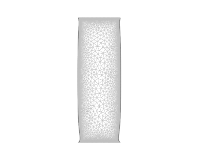
Figure 1: Final 2-D shape obtained by the gradient algorithm

4.2 Some 3D computations

In this section, we create a family of 2D shapes, constructed with cubic spline curves which look like the presumed optimum obtained in figure 1. Then, we obtain a family of 3D domains of volume $V$, by revolving the previous 2D shapes around the $(Ox_{3})$ axis. We introduce a small parameter $e$ in the control points of the cubic splines and we evaluate for each value of $e$ the criterion $J$. The value $e=0$ corresponds to the cylinder. Let us respectively denote by $J(e)$ and $J(\Omega_{0})$ the values of the criterion $J$ evaluated at the domain corresponding to value $e$ of the parameter and at the cylinder. Figure 2 is the plot of function $e\mapsto 100.\frac{J(e)-J(\Omega_{0})}{J(\Omega_{0})}$ above, and Figure 3 represents a better shape than the cylinder for the criterion $J$ which is obtained with a value of the parameter $e\simeq 0.001$. It shows that this simple method provides a 3D (axially symmetric) shape which is slightly better than the cylinder.

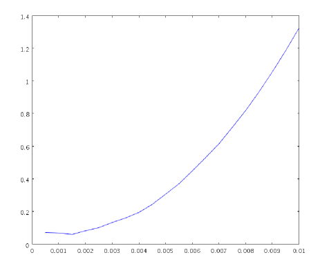
Figure 2: The cost function (which slightly decreases before increasing)

Figure 3: A 3D (axially symmetric) shape which is better than the cylinder

References

• [1] G. Allaire Shape optimization by the homogenization method, Applied Mathematical Sciences, 146, Springer-Verlag, New York, 2002.
• [2] G. Arumugam, O. Pironneau, On the problems of riblets as a drag reduction device, Optimal Control Appl. Methods 10 (1989), no. 2, 93–112.
• [3] F. Boyer, P. Fabrie, Eléments d’analyse pour l’étude de quelques modèles d’écoulements de fluides visqueux incompressibles, Mathématiques & Applications, vol. 52, Springer-Verlag, Berlin, 2006.
• [4] D. Chenais, On the existence of a solution in a domain identification problem, J. Math. Anal. Appl., 52 (1975), 189-289.
• [5] M. Delfour, J.P. Zolésio Shapes and geometries. Analysis, differential calculus, and optimization, Advances in Design and Control SIAM, Philadelphia, PA, 2001.
• [6] G. Dogğan, P. Morin, R.H. Nochetto, M. Verani Discrete gradient flows for shape optimization and applications, Computer methods in Applied Mechanics and Engineering, 2007.
• [7] E. Feireisl, Shape optimization in viscous compressible fluids, Appl. Math. Optim., 47 (2003), no. 1, 59–78.
• [8] G. P. Galdi An Introduction to the Mathematical Theory of the Navier-Stokes Equations Volumes 1 and 2, Springer Tracts in Natural Philosophy , Vol. 38, 1998
• [9] A. Henrot, M. Pierre, Variation et Optimisation de formes, coll. Mathématiques et Applications, vol. 48, Springer 2005.
• [10] A. Henrot, Y. Privat, Une conduite cylindrique n’est pas optimale pour minimiser l’énergie dissipée par un fluide, C. R. Acad. Sci. Paris Sér. I Math, (2008),
• [11] B. Mohammadi, O. Pironneau, Applied shape optimization for fluids, Clarendon Press, Oxford 2001.
• [12] C.B. Morrey, Multiple integrals in the calculus of variations, Springer, Berlin/Heidelberg/New York 1966.
• [13] F. Murat, J. Simon, Sur le contrôle par un domaine géométrique, Publication du Laboratoire d’Analyse Numérique de l’Université Paris 6, 189, 1976.
• [14] O. Pironneau, Optimal shape design for elliptic systems, Springer Series in Computational Physics, Springer, New York 1984.
• [15] O. Pironneau, G. Arumugam, On riblets in laminar flows, Control of boundaries and stabilization (Clermont-Ferrand, 1988), 53–65, Lecture Notes in Control and Inform. Sci., 125, Springer, Berlin, 1989.
• [16] P. Plotnikov, J. Sokolowski, Domain Dependence of Solutions to Compressible Navier-Stokes Equations, SIAM J. Control Optim., Volume 45, Issue 4, pp. 1165-1197.
• [17] Y. Privat, Quelques problèmes d’optimisation de formes en sciences du vivant, phD thesis of the University of Nancy, october 2008.
• [18] J. Sokolowski et J. P. Zolesio, Introduction to Shape Optimization Shape Sensitivity Analysis, Springer Series in Computational Mathematics, Vol. 16, Springer, Berlin 1992.
• [19] R. Temam Navier-Stokes Equations, North-Holland Pub. Company (1979), 500 pages.