Non binary LDPC codes over the binary erasure channel: density evolution analysis

Abstract

In this paper we present a thorough analysis of non binary LDPC codes over the binary erasure channel. First, the decoding of non binary LDPC codes is investigated. The proposed algorithm performs “on-the fly” decoding, i.e. it starts decoding as soon as the first symbols are received, which generalizes the erasure decoding of binary LDPC codes. Next, we evaluate the asymptotical performance of ensembles of non binary LDPC codes, by using the density evolution method. Density evolution equations are derived by taking into consideration both the irregularity of the bipartite graph and the probability distribution of the graph edge labels. Finally, infinite-length performance of some ensembles of non binary LDPC codes for different edge label distributions are shown.

I Introduction

Data loss recovery – for instance, for content distribution applications or for distributed storage systems – is widely addressed using FEC (Forward Error Correction) techniques based on error correcting codes. These codes are dealing with erasure channels, i.e. a channel that either transmits the data unit correctly (without error) or erases it completely. In the case of content distribution applications, the potential physical layer CRC, or physical layer FEC codes, or transport level UDP checksums, may lead a receiver to discard erroneous data units. For distributed storage systems, data loss may be due to broken servers, Denial-of-Service (DoS) attacks, etc.

The performance of error correcting codes over erasure channels can be analyzed precisely, and a flurry of research papers have already addressed this issue. Low-density parity-check (LDPC) codes [1], [2] with iterative decoding [3] proved to perform very close to the channel capacity with reasonable complexity [4] [5]. Moreover, “rateless” codes that are capable of generating an infinite sequence of repair symbols were proposed in [6] [7]. LDPC codes were generalized by Tanner [8], by introducing the sparse graph representation and replacing the Single Parity Check (SPC) constraint nodes with error correcting block codes. Nowadays, these codes are known as GLDPC codes and were recently investigated for the BEC [9], [10], [11]. Over the past few years there has been an increased interest in non binary LDPC codes due to their enhanced correction capacity, but at this time only few works are dealing with the BEC [12],[13]. In this paper we give a thorough analysis of non binary LDPC codes over the BEC. The paper is organized as follows: in Section II we review some background on the construction of non binary LDPC codes. The decoding of non binary LDPC codes over the BEC is addressed in Section III. In Section IV we derive the density evolution equations taking into consideration both the irregularity of the bipartite graph and the probability distribution of the graph edge labels. Thresholds of some ensembles of non binary LDPC codes for different edge label distributions are shown in Section V.

II Non binary LDPC codes

We denote by ${\mathbb{F}}_{q}$ the Galois field with $q$ elements. For practical reasons, we will assume that $q$ is a power of $2$, even if this condition is not always necessary. Thus, we set $q=2^{p}$, where $p$ is the vector space dimension of ${\mathbb{F}}_{q}$ over ${\mathbb{F}}_{2}$ (each time we refer to ${\mathbb{F}}_{q}$ as a vector space, we consider its ${\mathbb{F}}_{2}$-vector space structure). We fix once for all an isomorphism of ${\mathbb{F}}_{2}$-vector spaces:

$${\mathbb{F}}_{2}^{p}\stackrel{{\scriptstyle\sim}}{{\rightarrow}}{\mathbb{F}}_{q}$$ (1)

and we say that $(b_{0},\dots,b_{p-1})\in{\mathbb{F}}_{2}^{p}$ are the constituent bits of the symbol $s\in{\mathbb{F}}_{q}$, if they correspond to each other by the above isomorphism.

Let $\mathbb{L}$ be a multiplicative group acting on the vector space ${\mathbb{F}}_{q}$. For instance, we may have:

• $\mathbb{L}={\mathbb{F}}_{q}^{*}$, acting on ${\mathbb{F}}_{q}$ via the internal field multiplication;

• $\mathbb{L}={\mathbf{M}}_{p}^{*}({\mathbb{F}}_{2})$, the multiplicative group of invertible $p\times p$ matrices, acting on ${\mathbb{F}}_{q}$ via the isomorphism ${\mathbb{F}}_{2}^{p}\stackrel{{\scriptstyle\sim}}{{\rightarrow}}{\mathbb{F}}_{q}$ from (1).

The action of $\mathbb{L}$ on ${\mathbb{F}}_{q}$ will always be denoted multiplicatively, that is:

$$\mathbb{L}\times{\mathbb{F}}_{q}\rightarrow{\mathbb{F}}_{q}:\ \ (h,s)\mapsto hs$$ (2)

For any matrix $H\in{\mathbf{M}}_{M,N}(\mathbb{L})$ one can define a code:

$${\mathcal{C}} = \ker(H)$$

$$= \{(s_{1},\dots,s_{N})\mid\sum_{n=1}^{N}h_{m,n}s_{n}=0,\ \forall m=1,\dots,M\}$$

If $\mathbb{L}={\mathbb{F}}_{q}^{*}$ acting on ${\mathbb{F}}_{q}$ via the internal field multiplication, then ${\mathcal{C}}$ is a ${\mathbb{F}}_{q}$-linear code, but this does not happen for general $\mathbb{L}$.

The Tanner graph associated with the code ${\mathcal{C}}$, denoted by ${\cal H}$, consists of $N$ variable nodes and $M$ check nodes representing the $N$ columns and the $M$ lines of the matrix $H$. A variable node and a check node are connected by an edge if the corresponding element of matrix $H$ is not zero. Each edge of the graph is labeled by the corresponding non zero element of $H$. Thus, from now on, we refer to the elements of ${\mathbb{L}}$ as labels. We also denote ${\cal H}(n)$ the set of check nodes connected to a given variable node $n\in\{1,2,\dots,N\}$, and by ${\cal H}(m)$ the set of variable nodes connected to a given check node $m\in\{1,2,\dots,M\}$.

II-A The binary image of a non binary code

Any sequence $(s_{1},\dots,s_{N})\in{\mathbb{F}}_{q}^{N}$ may be mapped into a binary sequence of length $Np$ via the isomorphism of (1). The binary sequences associated with the codewords $(s_{1},\dots,s_{N})\in{\mathcal{C}}$ constitute a linear binary code ${\mathcal{C}}_{\mbox{\rm\scriptsize bin}}\subseteq{\mathbb{F}}_{2}^{Np}$, which is called the binary image of ${\mathcal{C}}$. Moreover, the action (2) of the multiplicative label group ${\mathbb{L}}$ on ${\mathbb{F}}_{q}$ induces a group morphism from ${\mathbb{L}}$ into the group of vector space endomorphisms ${\mathcal{L}}_{{\mathbb{F}}_{2}}({\mathbb{F}}_{q},{\mathbb{F}}_{q})$, and identifying ${\mathbb{F}}_{q}$ and ${\mathbb{F}}_{2}^{p}$ via (1), we get a morphism:

$${\mathbb{L}}\rightarrow{\mathcal{L}}_{{\mathbb{F}}_{2}}({\mathbb{F}}_{q},{\mathbb{F}}_{q})\stackrel{{\scriptstyle\sim}}{{\rightarrow}}{\mathcal{L}}_{{\mathbb{F}}_{2}}({\mathbb{F}}_{2}^{p},{\mathbb{F}}_{2}^{p})={\mathbf{M}}_{p}({\mathbb{F}}_{2})$$ (4)

Replacing each coefficient of the matrix $H\in{\mathbf{M}}_{M,N}({\mathbb{L}})$ with its image under the above morphism, we obtain a binary matrix $H_{\mbox{\rm\scriptsize bin}}\in{\mathbf{M}}_{Mp,Np}({\mathbb{F}}_{2})$, which is simply the parity check matrix of the binary code ${\mathcal{C}}_{\mbox{\rm\scriptsize bin}}$. While the encoding may be performed using either the non binary code or its binary image, the iterative decoding of a non binary code on its binary image generally yields very poor performance.

III Decoding non binary LDPC codes

For general channels, several decoding algorithms for non binary LDPC codes were proposed in the literature [14], [15], [16]. Because of the BEC specificity, these algorithms are all equivalent over the BEC, and they can be described in a slightly different manner, as presented below.

III-A Decoding over the BEC

In this section we assume that a non binary LDPC code is used over BEC($\epsilon$) – the binary erasure channel with erasure probability $\epsilon$. Thus, the length $N$ sequence of encoded ${\mathbb{F}}_{q}$-symbols is mapped into the corresponding binary sequence of length $Np$, which is transmitted over the BEC, each bit from the binary sequence being erased with probability $\epsilon$. We say that a ${\mathbb{F}}_{q}$-symbol is :

• received, if all of its constituent bits are received;

• erased, if all of its constituent bits are erased by the channel;

• partially erased, if some of its constituent bits are erased by the channel and some others are received.

At the receiver part, the received bits are used to reconstruct the corresponding ${\mathbb{F}}_{q}$-symbols. The reconstruction may be complete, partial, or lacking, according to whenever the corresponding symbol is received, partially erased, or erased.

Let $n$ be a variable node of the Tanner graph and $s\in{\mathbb{F}}_{q}$. We say that the symbol $s$ is eligible at the variable node $n$, if the probability of the $n^{\mbox{\rm\scriptsize th}}$ transmitted symbol being $s$ is non zero. Tacking into consideration the channel output, the a priori set of eligible symbols, denoted by ${\mathscr{E}}_{n}$, consists of the symbols that fit with the received constituent bits (if any) of the $n^{\mbox{\rm\scriptsize th}}$ transmitted symbol. Thus :

• ${\mathscr{E}}_{n}={\mathbb{F}}_{q}$, if the symbol is erased,

• ${\mathscr{E}}_{n}\varsubsetneq{\mathbb{F}}_{q}$, if the symbol is partially erased,

• $\mbox{\rm card}({\mathscr{E}}_{n})=1$, if the symbol is received.

These sets constitute the a priori information of the decoder. They are iteratively updated by exchanging extrinsic messages between variable and check nodes in the graph. Each message is a subset of ${\mathbb{F}}_{q}$, representing a set of eligible symbols. Precisely, the message sent by a graph node on an outgoing edge is a set of eligible symbols, which is computed according to messages received by the same node on the incoming edges. We use the following notation:

• ${\mathscr{A}}_{m,n}$ the set of eligible symbols sent by the variable node $n$ to the check node $m$;

• ${\mathscr{B}}_{m,n}$ the set of eligible symbols sent by the check node $m$ to the variable node $n$.

Finally, if ${\mathscr{S}},{\mathscr{S}}_{1},{\mathscr{S}}_{2}\subseteq{\mathbb{F}}_{q}$ and $h\in{\mathbb{L}}$ we define:

$$\begin{array}[]{rcl}h{\mathscr{S}}&=&\{hs\mid s\in{\mathscr{S}}\}\\ {\mathscr{S}}_{1}+{\mathscr{S}}_{2}&=&\{s_{1}+s_{2}\mid s_{1}\in{\mathscr{S}}_{1},s_{2}\in{\mathscr{S}}_{2}\}\end{array}$$

The iterative decoder for the BEC can be expressed as follows:

Initialization step

• variable-to-check messages initialization

  ${\mathscr{A}}_{m,n}={\mathscr{E}}_{n}$

Iteration step

• check-to-variable messages

  ${\mathscr{B}}_{m,n}=\displaystyle\sum_{n^{\prime}\in{\mathcal{H}}(m)\setminus\{n\}}h_{m,n^{\prime}}{\mathscr{A}}_{m,n^{\prime}}$

  
  

• variable-to-check messages

  ${\mathscr{A}}_{m,n}=\displaystyle{\mathscr{E}}_{n}\cap\left(\bigcap_{m^{\prime}\in{\mathcal{H}}(n)\setminus\{m\}}h_{m^{\prime},n}^{-1}{\mathscr{B}}_{m^{\prime},n}\right)$

  
  

• a posteriori sets of eligible symbols

  $\overline{{\mathscr{E}}}_{n}=\displaystyle{\mathscr{E}}_{n}\cap\left(\bigcap_{m\in{\mathcal{H}}(n)}h_{m,n}^{-1}{\mathscr{B}}_{m,n}\right)$

The decoder stops when all the a posteriori sets of eligible symbols $\overline{{\mathscr{E}}}_{n}$ are of cardinality $1$, or when a maximum number of iterations is reached. It is important to note that any set of eligible symbols (${\mathscr{E}}_{n},{\mathscr{A}}_{m,n},{\mathscr{B}}_{m,n}$, or $\overline{{\mathscr{E}}}_{n}$) is a ${\mathbb{F}}_{2}$-affine sub-space of ${\mathbb{F}}_{q}$; in particular, its cardinal is a power of $2$.

III-B Minimum-delay decoding

In this section we propose a minimum-delay decoding algorithm over the BEC, in the sense that the decoding starts since the reception of the first bits, which is suited for Upper-Layer Forward Error Correction (UL-FEC).

The minimum-delay decoding of non binary codes consists of removing symbols from the sets of eligible symbols:

• initialize ${\mathscr{E}}_{n}={\mathbb{F}}_{q}$, $n=1,\dots,N$

• each time a new bit is received, identify the variable node $n$ of which the received bit is a constituent bit, and then:

  A($n$):

  remove symbols from ${\mathscr{E}}_{n}$ whose corresponding constituent bit is different from the received bit

  B($n$):

  process the check nodes $m\in{\mathcal{H}}(n)$, then update the sets of eligible symbols ${\mathscr{E}}_{n^{\prime}}\leftarrow\overline{{\mathscr{E}}}_{n^{\prime}}$, for each $n^{\prime}\in{\mathcal{H}}(m)\setminus\{n\}$

  C($n$):

  For each of the above $n^{\prime}$s, if by updating ${\mathscr{E}}_{n^{\prime}}$ its cardinal has been reduced, go to B($n\leftarrow n^{\prime}$).

The decoder stops when all the sets ${\mathscr{E}}_{n}$ are of cardinality $1$.

III-B1 Decoding inefficiency

It follows that the minimum-delay decoding is actually an on-the-fly implementation of the previous iterative decoding. A performance metric that is often associated with on-the-fly decoding is the decoding inefficiency, defined as the ratio between the number of received bits before decoding stops and the number of information bits. Let $K_{\mbox{\rm\scriptsize bin}}$ be the binary dimension of the code, and $K_{\mbox{\rm\scriptsize received}}$ be the number of received bits before decoding stops. Then the inefficiency $\mu$ is defined as:

$$\mu=\frac{K_{\mbox{\rm\scriptsize received}}}{K_{\mbox{\rm\scriptsize bin}}}$$ (5)

The expectation of the random variable $\mu$, denoted by $\mu_{m}$, is called average inefficiency. In practice $\mu_{m}$ can be estimated by Monte-Carlo simulation.

The average inefficiency of the on-the-fly decoding can be related to the failure probability of the iterative decoding (section III). Precisely, for any $\epsilon\in[0,1]$, let $p(\epsilon)$ be the failure probability of the iterative decoding assuming that $\epsilon$ is the channel erasure probability. Assuming that the function $p$ is integrable on $[0,1]$, we have:

$$\mu_{m}-1=\int_{0}^{1}p(\epsilon)\,d\epsilon$$ (6)

IV Density evolution

Density evolution for non binary LDPC codes over the BEC was already derived in [12], assuming an uniform distribution on the edge labels. In loc. cit., the authors suggest that the distribution of the edge labels represents a degree of freedom that should be integrated to our understanding of capacity approaching iterative coding schemes. To do so, we derive the density evolution of non binary codes tacking into consideration the variable and check nodes degree distributions, but also the probability distribution of the edge labels. We use the following notation:

• $\lambda_{d}$ is the fraction of edges connected to variable nodes of degree $d$, $\lambda(X)=\displaystyle\sum_{d=1}^{d_{v}}\lambda_{d}X^{d-1}$ is the polynomial of variable node degree distribution;

• $\rho_{d}$ is the fraction of edges connected to check nodes of degree $d$, $\rho(X)=\displaystyle\sum_{d=1}^{d_{c}}\rho_{d}X^{d-1}$ is the polynomial of check node degree distribution;

• $f:{\mathbb{L}}\rightarrow[0,1]$ the probability distribution function defined by $f(h)=$ fraction of edges with label $h\in{\mathbb{L}}$. By extending the notation, for a given sequence ${\mathbf{h}}=(h_{1},\dots,h_{I})$ we define $f({\mathbf{h}})=\displaystyle\prod_{i=1}^{I}f(h_{i})$.

Without losing generality, we may assume that the all-zero codeword is transmitted. Thus, any set of eligible symbols (${\mathscr{E}}_{n},{\mathscr{A}}_{m,n},{\mathscr{B}}_{m,n}$, or $\overline{{\mathscr{E}}}_{n}$) is a ${\mathbb{F}}_{2}$-linear sub-spaces of ${\mathbb{F}}_{q}$. Table I gives the list of the possible values of the a priori sets of eligible symbols ${\mathscr{E}}_{n}$ for the case of a ${\mathbb{F}}_{8}$-code, according to the received binary sequence.

TABLE I: Possible values of the a priori sets of eligible symbols

$$\begin{array}[]{|c|c|c|}\hline\cr\mbox{received bits}^{*}&{\mathscr{E}}_{n}&\Pr({\mathscr{E}}_{n})\\ \hline\cr\hline\cr\mbox{x}\mbox{x}\mbox{x}&{\mathbb{F}}_{8}&\epsilon^{3}\\ \hline\cr 0\mbox{x}\mbox{x}&\{0,1,2,3\}&\epsilon^{2}(1-\epsilon)\\ \hline\cr\mbox{x}0\mbox{x}&\{0,1,4,5\}&\epsilon^{2}(1-\epsilon)\\ \hline\cr\mbox{x}\mbox{x}0&\{0,2,4,6\}&\epsilon^{2}(1-\epsilon)\\ \hline\cr\mbox{x}00&\{0,4\}&\epsilon(1-\epsilon)^{2}\\ \hline\cr 0\mbox{x}0&\{0,2\}&\epsilon(1-\epsilon)^{2}\\ \hline\cr 00\mbox{x}&\{0,1\}&\epsilon(1-\epsilon)^{2}\\ \hline\cr 000&\{0\}&(1-\epsilon)^{3}\\ \hline\cr\end{array}$$

^∗ Symbol x denotes an erased bit

Let $\mbox{\rm Gr}({\mathbb{F}}_{q})$ be the Grassmannian of ${\mathbb{F}}_{q}$, that is the set of all ${\mathbb{F}}_{2}$-linear subspaces of ${\mathbb{F}}_{q}$. For $V\in\mbox{\rm Gr}({\mathbb{F}}_{q})$, we note:

$$P_{\ell}(V) = \Pr({\mathscr{A}}_{m,n}^{(\ell)}=V)$$ (7)

$$Q_{\ell}(V) = \Pr({\mathscr{B}}_{m,n}^{(\ell)}=V)$$ (8)

where superscript $(\ell)$ is used to denote sets of eligible symbols computed at the $\ell^{\mbox{\rm\scriptsize th}}$ iteration. Thus, the decoding is successfully if and only if:

$$\lim_{\ell\rightarrow+\infty}P_{\ell}(\{0\})=1$$ (9)

In order to simplify the notation, we define:

• For any $V\in\mbox{\rm Gr}({\mathbb{F}}_{q})$:

  $$\begin{array}[]{r@{\ }c@{\ }l}\gamma(V)&{:}{=}&P_{0}(V)=\Pr({\mathscr{E}}_{n}=V)\\ {\mathcal{S}}_{V}^{(I)}&{:}{=}&\{{\underline{\mathbf{V}}}=(V_{1},\dots,V_{I})\mid\displaystyle\sum_{i=1}^{I}V_{i}=V\}\subseteq\mbox{\rm Gr}({\mathbb{F}}_{q})^{I}\\ {\mathcal{I}}_{V}^{(I)}&{:}{=}&\{(V_{0},{\underline{\mathbf{V}}})=(V_{0},V_{1},\dots,V_{I})\mid\displaystyle\bigcap_{i=0}^{I}V_{i}=V\}\\ &\subseteq&\mbox{\rm Gr}({\mathbb{F}}_{q})^{I+1}\end{array}$$

• For any ${\mathbf{h}}=(h_{1},\dots,h_{I})\in{\mathbb{L}}^{I}$ and ${\underline{\mathbf{V}}}=(V_{1},\dots,V_{I})\in\mbox{\rm Gr}({\mathbb{F}}_{q})^{I}$:

  $${\mathbf{h}}^{-1}{:}{=}(h_{1}^{-1},\dots,h_{I}^{-1}),\ \ {\mathbf{h}}\cdot{\underline{\mathbf{V}}}{:}{=}(h_{1}V_{1},\dots,h_{I}V_{I})$$

• For any ${\underline{\mathbf{V}}}=(V_{1},\dots,V_{I})\in\mbox{\rm Gr}({\mathbb{F}}_{q})^{I}$:

  $$P_{\ell}({\underline{\mathbf{V}}}){:}{=}\prod_{i=1}^{I}P_{l}(V_{i}),\ \ Q_{\ell}({\underline{\mathbf{V}}}){:}{=}\prod_{i=1}^{I}Q_{l}(V_{i})$$

Let $(m,n)$ be an edge of the tanner graph. Assume that ${\mathcal{H}}(m)=\{n,n_{1},\dots,n_{d-1}\}$, where $d$ is the degree of the check node $m$. To simplify the notation, we set $h_{i}=h_{m,n_{i}}$, the non zero label of the edge $(m,n_{i})$, for $i=1,\dots,d-1$. The probability of ${\mathscr{B}}_{m,n}^{(\ell+1)}$ being equal to $V$, conditioned on ${\mathbf{h}}=(h_{1},\dots,h_{d-1})$, may be computed as:

$$\Pr({\mathscr{B}}_{m,n}^{(\ell+1)}=V\mid{\mathbf{h}})=\sum_{{\underline{\mathbf{V}}}\in{\mathcal{S}}_{V}^{(d-1)}}\left(\ \prod_{i=1}^{d-1}P_{\ell}(h_{i}^{-1}V_{i})\ \right)$$ (10)

Averaging over all possible label sequences ${\mathbf{h}}$ we get:

$$Q_{\ell+1}^{(d-1)}(V) {:}{=} \Pr({\mathscr{B}}_{m,n}^{(\ell+1)}=V)$$ (11)

$$= \sum_{{\mathbf{h}}\in{\mathbb{L}}^{d-1}}\left(f({\mathbf{h}})\cdot\!\!\!\sum_{{\underline{\mathbf{V}}}\in{\mathcal{S}}_{V}^{(d-1)}}\!\!\!\!\!P_{\ell}({\mathbf{h}}^{-1}\cdot{\underline{\mathbf{V}}})\right)$$

Averaging over all possible check node degrees $d$, we obtain:

$$Q_{\ell+1}(V)=\sum_{d=1}^{d_{c}}\left(\rho_{d}\cdot Q_{\ell+1}^{(d-1)}(V)\right)$$ (12)

Now, consider an edge $(n,m)$ of the Tanner graph, and let the variable node $n$ be of degree $d$ and ${\mathcal{H}}(n)=\{m,m_{1},\dots,m_{d-1}\}$. To simplify notation, we set $h_{i}=h_{m_{i},n}$, the non zero label of the edge $(n,m_{i})$, for $i=1,\dots,d-1$. The probability of ${\mathscr{A}}_{m,n}^{(\ell+1)}$ being equal to $V$, conditioned on ${\mathbf{h}}=(h_{1},\dots,h_{d-1})$, may be computed as:

$$\Pr({\mathscr{A}}_{m,n}^{(\ell+1)}=V\mid{\mathbf{h}})=\sum_{(V_{0},{\underline{\mathbf{V}}})\in{\mathcal{I}}_{V}^{(d-1)}}\left(\ \gamma(V_{0})\prod_{i=1}^{d-1}Q_{\ell+1}(h_{i}V_{i})\ \right)$$ (13)

Again, by averaging over all possible label sequences ${\mathbf{h}}$, it follows that:

$$P_{\ell+1}^{(d-1)}(V)\ {:}{=}\ \Pr({\mathscr{A}}_{m,n}^{(\ell+1)}=V)$$ (14)

$$= \sum_{{\mathbf{h}}\in{\mathbb{L}}^{d-1}}\left(f({\mathbf{h}})\cdot\sum_{(V_{0},{\underline{\mathbf{V}}})\in{\mathcal{I}}_{V}^{(d-1)}}\!\!\!\!\!\gamma(V_{0})Q_{\ell+1}({\mathbf{h}}\cdot{\underline{\mathbf{V}}})\right)$$

Finally, averaging over all possible variable node degrees $d$, we obtain:

$$P_{\ell+1}(V)=\sum_{d=1}^{d_{v}}\left(\lambda_{d}\cdot P_{\ell+1}^{(d-1)}(V)\right)$$ (15)

Proposition 1

Let $V,W\in\mbox{\rm Gr}({\mathbb{F}}_{q})$ and $h\in{\mathbb{L}}$ such that $W=hV$. Then:

$$Q_{\ell+1}^{(d-1)}(W) = \sum_{{\mathbf{h}}\in{\mathbb{L}}^{d-1}}\left(f(h\cdot{\mathbf{h}})\cdot\!\!\!\sum_{{\underline{\mathbf{V}}}\in{\mathcal{S}}_{V}^{(d-1)}}\!\!\!\!\!P_{\ell}({\mathbf{h}}^{-1}\cdot{\underline{\mathbf{V}}})\right)$$ (16)

$$P_{\ell+1}^{(d-1)}(W) =$$

$$\sum_{{\mathbf{h}}\in{\mathbb{L}}^{d-1}}\left(f(h\cdot{\mathbf{h}})\cdot\!\!\!\sum_{(V_{0},{\underline{\mathbf{V}}})\in{\mathcal{I}}_{V}^{(d-1)}}\!\!\!\!\!\gamma(V_{0})Q_{\ell+1}({\mathbf{h}}\cdot{\underline{\mathbf{V}}})\right)$$ (17)

where $h\cdot(h_{1},\dots,h_{d-1})=(hh_{1},\dots,hh_{d-1})$. In particular, if $f$ is the uniform distribution, then $Q_{\ell+1}^{(d-1)}(W)=Q_{\ell+1}^{(d-1)}(V)$ and $P_{\ell+1}^{(d-1)}(W)=P_{\ell+1}^{(d-1)}(V)$.

We say that $V$ and $W$ are conjugate if there exists $h\in{\mathbb{L}}$ such that $W=hV$ and denote by $\mbox{\rm Gr}({\mathbb{F}}_{q})/{\mathbb{L}}$ the quotient set of conjugation classes.

Corollary 2

Assume that $f$ is the uniform distribution and let $V\in\mbox{\rm Gr}({\mathbb{F}}_{q})$. Then $Q_{\ell}(V)$ and $P_{\ell}(V)$ depend only on the conjugation class of $V$ in $\mbox{\rm Gr}({\mathbb{F}}_{q})/{\mathbb{L}}$.

Corollary 3

Assume that $f$ is the uniform distribution and that $\mathbb{L}={\mathbf{M}}_{p}^{*}({\mathbb{F}}_{2})$, the multiplicative group of invertible $p\times p$ matrices, acting on ${\mathbb{F}}_{q}$ via the isomorphism ${\mathbb{F}}_{2}^{p}\stackrel{{\scriptstyle\sim}}{{\rightarrow}}{\mathbb{F}}_{q}$ from (1). Let $V\in\mbox{\rm Gr}({\mathbb{F}}_{q})$. Then $Q_{\ell}(V)$ and $P_{\ell}(V)$ depend only on the dimension of the vector space $V$.

The above corollaries may be used to simplify the density evolution formulas, assuming a uniform distribution of the graph edge labels. For instance, if $\mathbb{L}={\mathbf{M}}_{p}^{*}({\mathbb{F}}_{2})$, one can derive the same formulas as in [12].

V Thresholds

We denote by $E_{{\mathbb{F}}_{q},{\mathbb{L}}}(\lambda,\rho,f)$ the ensemble of LDPC codes over ${\mathbb{F}}_{q}$, with labels group ${\mathbb{L}}$, distribution degree polynomials $\lambda$ and $\rho$, and probability distribution of edge labels $f$. Whenever the Galois group ${\mathbb{F}}_{q}$ and the labels group ${\mathbb{L}}$ are subunderstood, we will simply use $E(\lambda,\rho,f)$. We also denote by ${p_{\mbox{\rm\scriptsize th}}}_{{\mathbb{F}}_{q},{\mathbb{L}}}(\lambda,\rho,f)$ (or simply $p_{\mbox{\rm\scriptsize th}}(\lambda,\rho,f)$) the threshold probability of the above ensemble, that is (see also (9)):

$$\vspace{-2mm}p_{\mbox{\rm\scriptsize th}}(\lambda,\rho,f)=\max\{\epsilon\mid\lim_{\ell\rightarrow+\infty}\!\!\!P_{\ell}(\{0\})=1\mbox{ on BEC}(\epsilon)\}$$ (18)

By fixing the polynomials of degree distribution $\lambda$ and $\rho$, the probability threshold $p_{\mbox{\rm\scriptsize th}}$ may be seen as a function of the probability distribution $f$. This is illustrated in Fig. 1 and Fig. 2. The Galois field is ${\mathbb{F}}_{4}$ and the labels group ${\mathbb{L}}={\mathbb{F}}_{4}^{*}$, acting of ${\mathbb{F}}_{4}$ by the internal field multiplication. The horizontal axes $f(1)$ and $f(2)$ represent the probabilities of edge labels being $1$ and $2$, respectively. Thus, the probability of edge labels being $3$ is given by $f(3)=1-f(1)-f(2)$. We drawn the surface representing $p_{\mbox{\rm\scriptsize th}}$ as function of $f(1)$ and $f(2)$. The top of the surface is plotted in red, the middle in green, and the bottom in blue. The two figures correspond to two couples $(\lambda,\rho)$ of degree distributions that were also considered in [12]. In Fig. 1 we fix $\lambda=X$ and $\rho=X^{2}$. The maximum $p_{\mbox{\rm\scriptsize th}}$ is obtained for the uniform distribution $f(1)=f(2)=f(3)=1/3$ and its value is equal to $0.5772$. The minimum $p_{\mbox{\rm\scriptsize th}}=0.5$ is obtained for the three distributions concentrated in a single label (such codes are equivalent to binary codes). In Fig. 2 we fix $\lambda(X)=X^{2}$ and $\rho(X)=X^{3}$. For the uniform distribution $f(1)=f(2)=f(3)=1/3$, the threshold $p_{\mbox{\rm\scriptsize th}}=0.6348$. The minimum $p_{\mbox{\rm\scriptsize th}}=0.6346$. The maximum $p_{\mbox{\rm\scriptsize th}}=0.6474$ is obtained for the three distributions concentrated in one single label.

These two examples highlight a more general phenomenon that we observed for other ensembles of codes, as shown for instance in Fig. 3. For a given Galois field ${\mathbb{F}}_{q}$, and given polynomials $\lambda$, and $\rho$, it is possible to find a probability distribution $\tilde{f}$ of edge labels, such that:

• edge labels are equal to $1$ with high probability (meaning that $\tilde{f}(1)$ is close to $1$)

• ${p_{\mbox{\rm\scriptsize th}}}_{{\mathbb{F}}_{q},{\mathbb{F}}_{q}^{*}}(\lambda,\rho,\tilde{f})\thickapprox\displaystyle\max_{f}{p_{\mbox{\rm\scriptsize th}}}_{{\mathbb{F}}_{q},{\mathbb{F}}_{q}^{*}}(\lambda,\rho,{f})$

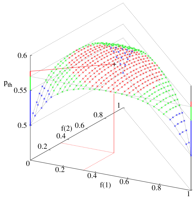
Figure 1: Probability threshold of the ensemble $E_{{\mathbb{F}}_{4},{\mathbb{F}}_{4}^{*}}(\lambda=X,\rho=X^{2},f)$ as function of labels probability distribution $f$.

$E_{{\mathbb{F}}_{8},{\mathbb{F}}_{8}^{*}}(\lambda,\rho,f)$

Labels pdf $f$ Threshold 1 2 3 4 5 6 7 1/7 1/7 1/7 1/7 1/7 1/7 1/7 0.4353 1/5 1/5 1/5 0 0 1/5 1/5 0.4356 1/3 0 0 1/3 0 0 1/3 0.4373 1/3 1/3 1/3 0 0 0 0 0.4391 1/2 0 0 0 0 0 1/2 0.4437 0.8 0 0 0 0 0 0.2 0.4483 0.9 0 0 0 0 0 0.1 0.436 0.95 0 0 0 0 0 0.05 0.4179 1 0 0 0 0 0 0 0.4

$E_{{\mathbb{F}}_{4},{\mathbb{F}}_{4}^{*}}(\lambda,\rho,f)$

Labels pdf $f$ Threshold 1 2 3 1/3 1/3 1/3 0.4487 1/2 1/2 0 0.4489 0.8 0.1 0.1 0.4507 0.9 0.07 0.03 0.4335 0.97 0.03 0 0.4121 1 0 0 0.4

Figure 3: Probability thresholds of the ensembles $E_{{\mathbb{F}}_{8},{\mathbb{F}}_{8}^{*}}(\lambda,\rho,f)$ and $E_{{\mathbb{F}}_{4},{\mathbb{F}}_{4}^{*}}(\lambda,\rho,f)$ for $\lambda=0.5X+0.5X^{4}$, $\rho=X^{5}$, and different labels probability distributions $f$.

For instance, considering the ensemble of codes over ${\mathbb{F}}_{8}$ from Fig. 3, if $\tilde{f}$ is defined by $\tilde{f}(1)=0.8$, $\tilde{f}(7)=0.2$, and $\tilde{f}(i)=0$ for $1<i<7$, then ${p_{\mbox{\rm\scriptsize th}}}_{{\mathbb{F}}_{8},{\mathbb{F}}_{8}^{*}}(\lambda,\rho,\tilde{f})=0.4483$. In this case only few Galois field multiplications are needed, and the decoder complexity is considerably reduced.

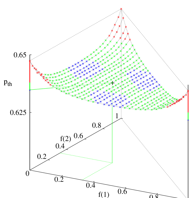
Figure 2: Probability threshold of the ensemble $E_{{\mathbb{F}}_{4},{\mathbb{F}}_{4}^{*}}(\lambda=X^{2},\rho=X^{3},f)$ as function of labels probability distribution $f$.

VI Conclusions

In this paper we investigated the decoding of non binary LDPC codes over the BEC, and we introduced a minimum-delay decoding suited for UL-FEC. We also derived the density evolution equations taking into consideration both the irregularity of the bipartite graph of the code and the probability distribution of the graph edge labels, giving a thorough understanding of the asymptotical behavior of ensembles of non binary LDPC codes. A non-uniform probability distribution of the edge labels might improve the decoder performance, but the most important advantage is that the decoder complexity can be significantly reduced. The design of capacity approaching non binary LDPC codes will be addressed in future works.

References

• [1] R. G. Gallager, Low Density Parity Check Codes, Ph.D. thesis, MIT, Cambridge, Mass., September 1960.
• [2] R. G. Gallager, Low Density Parity Check Codes, M.I.T. Press, 1963, Monograph.
• [3] V. Zyablov and M. Pinsker, “Decoding complexity of low-density codes for transmission in a channel with erasures,” Translated from Problemy Peredachi Informatsii, vol. 10(1), 1974.
• [4] T.J. Richardson, M.A. Shokrollahi, and R.L. Urbanke, “Design of capacity-approaching irregular low-density parity-check codes,” Information Theory, IEEE Transactions on, vol. 47, pp. 619–637, 2001.
• [5] M.G. Luby, M. Mitzenmacher, M.A. Shokrollahi, and D.A. Spielman, “Efficient erasure correcting codes,” IEEE Trans. Inf. Theory, vol. 47, no. 2, pp. 569–584, 2001.
• [6] M. Luby, “LT codes,” Proc. ACM Symp. Found. Comp. Sci., 2002.
• [7] A. Shokrollahi, “Raptor codes,” IEEE/ACM Trans. Networking (TON), vol. 14, pp. 2551–2567, 2006.
• [8] R. M. Tanner, “A recursive approach to low complexity codes,” IEEE Trans. Inform. Theory, vol. 27, no. 5, pp. 533–547, 1981.
• [9] E. Paolini, M. Fossorier, and M. Chiani, “Analysis of Generalized LDPC Codes with Random Component Codes for the Binary Erasure Channel,” Int. Symp. on Information Theory and its Applications (ISITA), 2006.
• [10] E. Paolini, M. Fossorier, and M. Chiani, “Generalized Stability Condition for Generalized and Doubly-Generalized LDPC Codes,” International Symposium on Information Theory (ISIT), 2007.
• [11] N. Miladinovic and M. Fossorier, “Generalized LDPC codes and generalized stopping sets,” IEEE Trans. on Comm., vol. 56(2), pp. 201–212, 2008.
• [12] V. Rathi and R. Urbanke, “Density Evolution, Thresholds and the Stability Condition for Non-binary LDPC Codes,” IEE Proc.-Commun., vol. 152, no. 6, 2005.
• [13] V. Rathi, “Conditional Entropy of Non-Binary LDPC Codes over the BEC,” International Symposium on Information Theory (ISIT), 2008.
• [14] N. Wiberg, Codes and decoding on general graphs, Ph.D. thesis, Likoping University, 1996, Sweden.
• [15] D. Declercq and M. Fossorier, “Extended min-sum algorithm for decoding LDPC codes over $\mbox{GF}(q)$,” in Information Theory, 2005. ISIT 2005. Proceedings. International Symposium on, 2005, pp. 464–468.
• [16] V. Savin, “Min-Max decoding for non binary LDPC codes,” in Information Theory, 2008 IEEE International Symposium on, 2008.