Oscillations and patterns in interacting populations of two species

Abstract

Interacting populations often create complicated spatiotemporal behavior, and understanding it is a basic problem in the dynamics of spatial systems. We study the two-species case by simulations of a host–parasitoid model. In the case of co-existence, there are spatial patterns leading to noise-sustained oscillations. We introduce a new measure for the patterns, and explain the oscillations as a consequence of a timescale separation and noise. They are linked together with the patterns by letting the spreading rates depend on instantaneous population densities. Applications are discussed.

A fundamental aim in studying population dynamics is to understand species interactions. A paradigmatic, still interesting, case is that of two species lot20 , where one feeds or lives from the other. These may be predators and their prey or parasitoids living on the expense of hosts. If the interaction is strong and if the parasitoid or predator is specialized, its growth will have a delayed negative feedback as its resource is diminished. In such cases, oscillations are an inherent feature bac41 . Many surface reactions also have similar dynamics zhdanov2002 .

The classical ways of looking at such systems assume fully stirred populations. The encounters between individuals are assumed to be proportional to the product of their densities, analogously to the mass action principle in chemistry lot20 . This assumption is also at the heart of the mean-field -like Lotka–Volterra equations. In general, however, spreading and interaction are restricted in space. In this case, correlated structures arise and the assumption about complete mixing no longer holds sol06 .

If the parasite abundance is small, any feedback effect is weak. Population sizes then show no oscillations, and the predating species is locally concentrated in a cluster-like arrangement. This has been theoretically studied in Ref. ova06 . With strong feedback spatiotemporal patterns emerge in a multitude of forms. These include disordered flame-like patterns tai94 ; zha06 ; mobilia07 , and ripple-like spatiotemporal ones ngu06 . There is also a large body of work on similar patterning in individual-based models (e.g. deroos91 ), in statistical physics szabo2002 ; woo06b , and in calcium concentration oscillations in living cells clapham98 . A paradigmatic pattern-forming system is the complex Ginzburg-Landau equation (CGLE) aranson2002 , which exhibits spiral-like geometries.

Voles in Northern Britain lam98 , mussels in the Wadden sea kop05 , and lemmings in Northern Europe han01 , are good examples of empirical observations of such patterning. These involve either predation or being predated. Spatial structures weaken the interactions since species tend to be aggregated within themselves. They also provide the prey a refuge since around the prey there are less predators. Therefore, spatial inhomogeneity can stabilize the dynamics and promote coexistence zha06 ; sol06 ; bri04 .

Here, we analyze the full spatiotemporal dynamics of two interacting species using instantaneous configurations and time series of the population densities. We introduce a measure for the level of patterning in such systems. When the patterns form, one observes persistent oscillations in the population densities. We show that the underlying dynamics follows a particular logic: it originates in the response of the rates to changes in instantaneous densities, and the emerging system proves different from the limit cycle in Lotka–Volterra systems, or recent developments where three-species models have been mapped reichenbach07 ; reichenbach08 to CGLE. The present mechanism works by the interplay of oscillatory transients to a stable fixed point and stochasticity. The response of the interaction rates is due to spatial correlations. The mechanism is novel, and does not in fact need any non-linearities to work, which will become evident below based on simulations and effective equations describing them.

We study a host–parasitoid model in discrete time and space. It is inspired by has91 , but has a wider interaction range as in the incidence function models of metapopulation dynamics (han98, ). The model describes annual host–parasitoid dynamics on a two-dimensional square lattice $\Lambda$ future . At each time step, a site ${\bf x}$ can be either empty (in state $e$) or populated by a host without (state $h$) or with parasitoids (state $p$). Transitions between the states are cyclic, $e\to h\to p\to e$, neglecting possible spontaneous deaths of non-parasitized hosts assumed to be rare, for simplicity. Although this means that hosts live forever if there are no parasitoids, this is not a serious restriction; in coexistence it boils down to assuming faster extinction for the parasitoids than for the hosts. The model can also be described as an SIR model with rebirth.

At each site transition probabilities depend on the surrounding populations through the connectivity

$$I_{\alpha}({\bf x},t)=\sum_{{\bf x^{\prime}}\in\Lambda}k_{\alpha}(|{\bf x}\!-\!{\bf x^{\prime}}|)\;\chi_{\alpha}({\bf x^{\prime}},t)$$ (1)

of site ${\bf x}$ with respect to species $\alpha$ ($h$ or $p$). Here $\chi_{\alpha}({\bf x})=1$ if the state of ${\bf x}$ is $\alpha$, and 0 else. The kernel $k_{\alpha}$ has an exponential decay with the scale $w_{\alpha}$ and is normalized by $\sum_{{\bf x}\in\Lambda}k_{\alpha}(|{\bf x}|)=1$. Dispersal lengths are chosen since these are biologically motivated han98 and lead to generalizability.

In a timestep, the transition $e\to h$ takes place with probability $\min(1,\lambda_{h}I_{h})$ and $h\to p$ with probability $\min(1,\lambda_{p}I_{p})$ (in the parameter range of interest, $\lambda_{\alpha}I_{\alpha}\leq 1$ practically always). Parasitized hosts may die ($p\to e$) with probability $\delta$ irrespective of the surroundings. Note that they do not reproduce. Periodic boundary conditions and parallel updates are used. There are two absorbing states, an empty lattice ($e$) and one full of hosts. Fig. 1 (a) shows an example with coexistence.

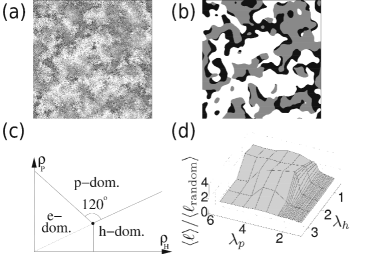
Figure 1: (a) Patterned co-existing configuration with parameters $w_{h}=3.0$, $w_{p}=1.5$, $\lambda_{h}=0.63$, $\lambda_{p}=2.5$, $\delta=0.9$, and $L=512$. Sites in $e$ are white, $h$ is gray, and $p$ black. (b) Dominance regions of the same state. (c) The definition of the coarse domains. For given $\bar{h}$ and $\bar{p}$, the first quadrant of the $(\rho_{h},\rho_{p})$-plane is divided into three regions by three lines. That separating $h$- and $p$-dominated regions starts from the average $(\bar{h},\bar{p})$ (the black dot), goes towards increasing $\rho_{h}$ and $\rho_{p}$ and is such that its continuation passes through the origin. The other two lines form 120-degree angles with the first one and each other. (d) The domain wall length ratio for different values of $\lambda_{h}$ and $\lambda_{p}$. Other parameters are $\delta=0.9$, $w_{h}=3.0$, $w_{p}=1.5$, $L=512$, and $\sigma=8$.

One finds moving regions predominantly in one of the three states. To quantify these patterns, we define the dominance regions (Fig. 1b) as follows. By smoothing one obtains continuous densities $\rho_{\alpha}({\bf x},t)=\sum_{{\bf x^{\prime}}\in\Lambda}\frac{1}{2\pi\sigma^{2}}e^{\frac{-|x-x^{\prime}|^{2}}{2\sigma^{2}}}\;\chi_{\alpha}({\bf x^{\prime}},t)$. For each site, $\rho_{h}({\bf x},t)$ and $\rho_{p}({\bf x},t)$ are compared to the space–time averages $\bar{h}$ and $\bar{p}$. The densities are positive, lying in the first quadrant of $\mathbb{R}^{2}$, divided into three regions shown in Fig. 1c. The site $x$ at time $t$ is then defined to belong to a domain according to the region ($e$, $h$, or $p$) containing $(\rho_{h}(x,t),\rho_{p}(x,t))$. In essence, the regions coarse-grain on a scale $\sigma>w_{h,p}$. In this regime, they are insensitive to changes in $\sigma$.

The domains are separated by walls, joining at triple points, vortices tai94 . A vortex has a sign $+1$ ($-1$), if one encounters the domains in the order $ehp$ following a small cycle around the vortex counter-clockwise (clockwise). Pairs of vortices of opposite signs are created and annihilated together. The domains rotate around the vortices, which are relatively stable. In other words, the species invade the appropriate neighboring domains so that the walls rotate around the vortices. Similar structures have been identified earlier in related systems (e.g. tai94 ; szabo2002 ). In three dimensions, the vortices generalize to strings tai94 .

First, consider static measures such as the domain wall length from source to sink vortex. It has an exponential distribution, whose mean is drawn for different parameters in Fig. 1d. Its ratio to its counterpart in uncorrelated random arrangements with the same densities is shown. Patterns and oscillations lead to walls with $\langle\ell\rangle\approx 100$ lattice units (l.u.). This is more than ten times larger than the smoothing width $\sigma$ and also several times that in the random arrangements ($\ell_{\rm random}=35$ l.u.). The coarse-graining gives a measure of patterns distinguishing between uncorrelated and patterned states.

Next, turn to the spatially averaged densities $h_{t}$ and $p_{t}$. Fig. 2a shows them as a function of time in three cases: (i) a non-patterned state with a small parasitoid population, (ii) a state with patterns, and (iii) a small subsystem ($L_{\rm sub}=64$) out of a large system ($L=512$) with patterns. In the patterned systems, there is a high-frequency oscillation matching the angular velocity of single vortices and a slow variation of the amplitude. Below, we explain both as a consequence of a timescale separation, connect them to the patterns, and explain why the oscillations do not conform to the usual limit cycles.

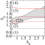
Figure 2: (a) Upper panel: the densities in the patterned state for $L=512$ (solid lines), and a subsystem with $L=64$ (dashed lines). See Fig. 1 for parameters. Lower panel: the same in the homogeneous state for $L=512$ and $\lambda_{p}=1.3$. The parasitoid curve has been shifted for clarity. (b) The phase diagram of the system. (1) Parasitoids extinct, (2) non-oscillatory coexistence, (3) coexistence with noise-sustained oscillations, (4) coexistence in a limit cycle, and (23) a transition zone between (2) and (3). Black (red) lines denote the boundaries for the spatial system (MF approximation). The boundary between (1) and (2) coincides for the two cases.

To build a description of the dynamics of the model in a novel fashion using aggregated variables, consider Poincaré maps (Fig. 3). For large enough systems $h_{t\!+\!1}$ and $p_{t\!+\!1}$ are unique functions of $h_{t}$ and $p_{t}$ up to noise. Also by attractor reconstruction pack80 we find that the full system with $2L^{2}$ degrees of freedom coarse-grains into a two-dimensional one. The points in the maps lie close to a two–dimensional surface, and for large enough $L$ (with many patterns in the system) even on the tangential plane through the average $(\bar{h},\bar{p})$. Based on these numerical observations, the dynamics is linear in $h_{t}$ and $p_{t}$:

$$h_{t\!+\!1} = a_{h,h}h_{t}+a_{h,p}p_{t}+c_{h}$$

$$p_{t\!+\!1} = a_{p,h}h_{t}+a_{p,p}p_{t}+c_{p}\,.$$ (2)

In other words, the observations imply that even though the dynamics is expected to be non-linear based on the MF approximation, in a large system with many patterns the possible non-linearities self-average out.

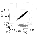
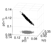
Figure 3: Left: $h_{t\!+\!1}$ over $h_{t}$ and $p_{t}$ (black) in a perspective showing the planar arrangement of points and its projection onto the $(h_{t},p_{t})$-plane (gray). Right: the same for $p_{t+1}$. Parameters are as in Fig. 1.

It is then useful to consider the expansion around the average – a linear iterative map. In oscillatory cases, its eigenvalues form a conjugated pair $\rho e^{\pm i\phi}$. These are associated with two timescales, the period and the decay rate of the amplitude. Their ratio

$$\nu\equiv\phi/|\log\rho|$$ (3)

tells whether dynamics is oscillatory or “just noisy”. $\nu\gg 1$ indicates patterned systems and oscillatory dynamics. Fig. 4 shows the typical behaviors of the two kinds of dynamics observed depending on the presence or absence of patterns, and whether one adds noise (as additional Gaussian uncorrelated noise terms on the RHS of Eq. (2)) to the coarse-grained dynamical system to mimic the finite-$L$ simulations of the full spatial system. Note that in all cases the fixed point is attractive.

Figure 4: The behavior of Eqs. (2) in the patterned (a, b, c) and in the homogeneous state (d, e, f). The coefficients $a_{\sigma,\sigma^{\prime}}$ and $c_{\sigma}$ are obtained from fits of Eq. (2) to simulation data. In both cases they lead to an oscillatory convergence to the FP (a, d). With noise, the FP is never reached and the cases differ: in the homogeneous one this results in random fluctuations around the FP (e); in the patterned case the noise kicks the system out of the FP with slow and oscillatory decay and leads to persistent oscillations different from limit cycles (b). The host density as a function of time corresponding to (b, e) is shown in (c, f).

So far we have given separately a temporal and a spatial diagnosis of the pattern dynamics. Next we link these together. For $\lambda_{\alpha}I_{\alpha}({\bf x},t)$ small, they equal the spreading probabilities, and the dynamics can be written as $h_{t+1}=\!h_{t}+\!\!\sum_{{\bf x}\in\Lambda}\!\Bigl{[}\lambda_{h}k_{h}({\bf x})C_{eh}({\bf x},t)-\lambda_{p}k_{p}({\bf x})C_{hp}({\bf x},t)\Bigr{]}$ and $p_{t+1}=(1\!-\!\delta)p_{t}+\lambda_{p}\sum_{{\bf x}\in\Lambda}k_{p}({\bf x})\;C_{hp}({\bf x},t)$, where the influence of the connectivities is expressed by the correlation functions $C_{\alpha\beta}({\bf x},t)=\frac{1}{|\Lambda|}\sum_{{\bf x^{\prime}}\in\Lambda}\chi_{\alpha}({\bf x^{\prime}},t)\;\chi_{\beta}({\bf x}+{\bf x^{\prime}},t)$. A corresponding non-spatial approximation is

$$h_{t\!+\!1} = h_{t}+\kappa(h_{t},p_{t})(1\!-\!h_{t}\!-\!p_{t})h_{t}-\mu(h_{t},p_{t})h_{t}p_{t}$$

$$p_{t\!+\!1} = (1-\delta)p_{t}+\mu(h_{t},p_{t})h_{t}p_{t}\,.$$ (4)

This is an approximation of the usual MF form with the interaction parameters $\kappa(h,p)$ and $\mu(h,p)$ generalized to be arbitrary functions of the instantaneous densities. They can be non-linear and they do not have to conform to the standard MF nor to any ad-hoc approximations pas01 . By an expansion of Eqs. (4) around the fixed point $(\bar{h},\bar{p})$ one arrives at Eq. (2) with

$$a_{h,h} = 1\!+\!\kappa\!-\!2\kappa\bar{h}\!-\!(\kappa\!+\!\mu)\bar{p}\!+\!\partial_{h}\kappa\,\bar{h}(1\!-\!\bar{h}\!-\!\bar{p})-\partial_{h}\mu\,\bar{h}\bar{p}$$

$$a_{h,p} = -(\kappa\!+\!\mu)\bar{h}-\partial_{p}\kappa\;\bar{h}(1\!-\!\bar{h}\!-\!\bar{p})-\partial_{p}\mu\;\bar{h}\bar{p}$$

$$a_{p,h} = \mu\bar{p}+\partial_{h}\mu\;\bar{h}\bar{p}$$ (5)

$$a_{p,p} = 1-\delta+\mu\bar{h}+\partial_{p}\mu\;\bar{h}\bar{p},$$

where $\kappa$, $\mu$, and their derivatives are evaluated at the fixed point. The derivatives are necessary for consistency. The matrix elements $a_{\sigma,\sigma^{\prime}}$ and the densities $\bar{h}$ and $\bar{p}$ are measured from the simulations. Since $\kappa$ and $\mu$ are parameters, omitting the derivatives would make Eqs. (5) overdetermined and thus unsatisfiable. By keeping them, there are four equations and four unknowns to be solved.

The effect of the nonzero derivatives is best illustrated by a phase diagram, Fig. 2. In the spatially extended system, there are three qualitative phases: the extinction of the parasitoids, non-oscillatory and oscillatory coexistence. Except for the extinction, the boundaries are not sharp. Instead, there is a transition zone, defined via the timescale ratio (Eq. (3)) as the region where $1\!<\!\nu\!<\!4$. In MF, there is also a fourth phase, absent here: oscillatory coexistence in a limit cycle. The phase structure resembles that in earlier work on a related model with only nearest-neighbour spreading satulovsky1994 ; tome2007 ; arashiro2008 . There, as well, oscillatory and non-oscillatory phases are recovered, the latter identified as a limit cycle using the pair approximation. Based on our findings, it could also be noise-sustained.

Let us now compare the explained mechanism with recent approaches. A possibility is to make the angular velocity of the oscillation either amplitude- or phase-dependent (abt07prl, ; abt07pre, ). However, Eq. (2) does not allow for either dependence. Another one is to map the population model reichenbach07 ; reichenbach08 to CGLE aranson2002 . An unstable fixed point is necessary for the mapping, yielding a limit cycle.

To conclude, we have studied spatiotemporal dynamics of a model of two kinds of interacting particles, in biological terms hosts and parasitoids. A large parasitoid population creates patterns and noisy oscillations of population sizes. We have introduced a new measure for the patterns, and explained the noisy oscillation as a consequence of a time-scale separation. In other words, even with a limit cycle at the well-mixed limit, the spatial case has stable dynamics with long-lived oscillatory transients. This is due to spatial correlations making the spreading rates functions of the instantaneous population densities. Since the type of oscillation determines its properties (e.g. the fluctuating amplitude), which in turn affect vulnerability to extinction, the distinction is important. The connection offers a shortcut to study the effect of, e.g. environment: it could be related directly to the matrix elements in (2), in contrast to a full form of the interactions, lightening the analysis. We expect that the observation of patterns and oscillations arising from local dynamics and self-averaging - in finite systems since the noise amplitude depends on system size - will find other applications beyond the biology-inspired model. They are not restricted to only two species or two-dimensional systems, since the analysis can be carried out also for more complicated cases. There is no restriction to cyclic dynamics either, nor to discrete-time systems since continuous-time ones can be handled by considering snapshots taken at regular intervals. Further examples of applications include chemical reactions on surfaces zhdanov2002 , and metapopulations on disordered and scalefree landscapes.

Acknowledgments. Ilkka Hanski and Otso Ovaskainen are thanked for stimulating discussions and Lasse Laurson for assistance. This work was supported by the Academy of Finland through the Center of Excellence program (M.A. and M.P.) and Deutsche Forschungsgemeinschaft via SFB 611 (M.R.). The authors thank the Lorentz center for kind hospitality.

References

- (1) A.J. Lotka, J. Am. Chem. Soc. (1920).
- (2) P. De Bach and H.S. Smith, Ecology 22, 363 (1941).
- (3) V. P. Zhdanov, Surf. Sci. Rep. 45, 231 (2002).
- (4) R.V. Solé and J. Bascompte, Self-Organization in Complex Ecosystems, Princeton University Press, Princeton (2006).
- (5) O. Ovaskainen and S. Cornell, Proc. Natl. Acad. Sci. 103, 12781 (2006).
- (6) K.-i. Tainaka, Phys. Rev. E 50, 3401 (1994).
- (7) F. Zhang, Z. Li, and C. Hui, Ecological Modelling 193, 721 (2006).
- (8) M. Mobilia and I. T. Georgiev and U. C. Täuber, J. Stat. Phys. 182, 447 (2007).
- (9) T. Nguyen-Huu, C. Lett, J.C. Poggiale, and P. Auger, Ecological Modelling 197, 290 (2006).
- (10) A. M. de Roos, E. McCauley, and W. G. Wilson, Proc. Biol. Sci. 246, 117 (1991).
- (11) G. Szabó and A. Szolnoki, Phys. Rev. E 65, 036115 (2002).
- (12) K. Wood, C. Van den Broeck, R. Kawai, and K. Lindenberg, Phys. Rev. Lett. 96, 145701 (2006).
- (13) D. E. Clapham, Cell 80, 259 (1998).
- (14) I. S. Aranson and L. Kramer, Rev. Mod. Phys. 74, 99 (2002).
- (15) X. Lambin, D.A. Elston, S.J. Petty, and J.L. MacKinnon, Proc. R. Soc. Lond. B 265, 1491 (1998).
- (16) J. van de Koppel, M. Rietkerk, N. Dankers, and P.M.J. Herrman, Am. Nat. 165, E66 (2005).
- (17) I. Hanski, H. Henttonen, E. Korpimäki, L. Oksanen, and P. Turchin, Ecology 82, 1505 (2001).
- (18) C. Briggs and M.F. Hoopes, Theor. Pop. Biol. 65, 299 (2004).
- (19) T. Reichenbach, M. Mobilia, and E. Frey, Nature 448, 1046 (2007).
- (20) T. Reichenbach, M. Mobilia, and E. Frey, e-print, arXiv:0801.1798.
- (21) M.P. Hassell, H.N. Comins, and R.M. May, Nature 353, 255 (1991).
- (22) I. Hanski, Nature 396, 41 (1998).
- (23) One can also study in a similar way a realistic example of a metapopulation landscape, the Åland archipelago on the Baltic Sea (manuscript in preparation).
- (24) N.H. Packard, J.P. Crutchfield, J.D. Farmer, and R.S. Shaw, Phys. Rev. Lett. 45, 712 (1980).
- (25) M. Pascual, P. Mazzega, and S.A. Levin, Ecology 82, 2357 (2001).
- (26) J.E. Satulovsky and T. Tomé, Phys Rev. E 49, 5073 (1994).
- (27) T. Tomé and K.C. de Carvalho, J. Phys. A Math. Gen. 40, 12901 (2007).
- (28) E. Arashiro, A. L. Rodrigues, M. J. de Oliveira, and T. Tomé, Phys. Rev. E 77, 061909 (2008).
- (29) R. Abta, M. Schiffer, and N. M. Shnerb, Phys. Rev. Lett. 98, 098104 (2007).
- (30) R. Abta and N. M. Shnerb, Phys. Rev. E 75, 051914 (2007).